Validating Autofocus Algorithms with Automated Tests

1
User Centred Technologies Research, University of Applied Sciences Vorarlberg, 6850 Dornbirn, Austria
2
WolfVision GmbH, 6833 Klaus, Austria
*
Author to whom correspondence should be addressed.
Robotics 2018, 7(3), 33; https://doi.org/10.3390/robotics7030033
Submission received: 27 March 2018
/
Revised: 15 June 2018
/
Accepted: 20 June 2018
/
Published: 25 June 2018
(This article belongs to the Special Issue Intelligent Systems in Robotics)
Abstract
:For an automated camera focus, a fast and reliable algorithm is key to its success. It should work in a precisely defined way for as many cases as possible. However, there are many parameters which have to be fine-tuned for it to work exactly as intended. Most literature only focuses on the algorithm itself and tests it with simulations or renderings, but not in real settings. Trying to gather this data by manually placing objects in front of the camera is not feasible, as no human can perform one movement repeatedly in the same way, which makes an objective comparison impossible. We therefore used a small industrial robot with a set of over 250 combinations of movement, pattern, and zoom-states to conduct these tests. The benefit of this method was the objectivity of the data and the monitoring of the important thresholds. Our interest laid in the optimization of an existing algorithm, by showing its performance in as many benchmarks as possible. This included standard use cases and worst-case scenarios. To validate our method, we gathered data from a first run, adapted the algorithm, and conducted the tests again. The second run showed improved performance.
1. Introduction
The idea of our study was to optimize the automated focus algorithm—in this case, a variation of the contrast detection method [1]—of a product for its performance in various scenarios. As the system was a high-end product in the document digitalization and presentation business, usability and user experience were very important. According to Shneiderman, Plaisant, Cohen, Jacobs, Elmqvist, and Diakopoulos [2], the first of their “8 golden rules for usability” is to “strive for consistency”. Also according to them, systems that cannot do their work will not be used, whereas systems that work faster than others will be preferred. To improve the system appropriately, it became necessary to test the algorithm in a wide range of objective scenarios, which could then be interpreted by the respective developers. We generated a dataset of 294 scenarios, attempting to simulate as many actual use cases for the camera as possible. They were the product of 14 movements, 7 patterns, and 3 zoom levels. Reliability and speed were the two most important factors for the autofocus algorithm [3,4,5]. As manual validation of these scenarios was unfeasible, i.e., humans are unable to exactly repeat the various movements, we developed a setup which could be used to benchmark different versions of the algorithm of the camera. To achieve this, we equipped a robot adequately and programmed it to do the movements typical for presentation tasks while logging the state of the lenses on a computer. The basic idea itself was very similar to that of Bi, Pomalaza-Ráez, Hershberger, Dawson, Lehman, Yurek, and Ball [6] who used automated actuators to test electrical cable harnesses and logged the resulting signals on an external station. As opposed to their tests of wires with a simple fail/pass result, we also needed to classify the resulting data accordingly. The results from a first measurement confirmed our assumption of scenarios where deficits existed. This knowledge was used to change the parameters of the autofocus, striving for more consistency. Adapting the algorithm appropriately led to an improved performance in the second measurement.
Related Works
Concerning the autofocus, several papers were of interest, however they turned out to not be applicable due to our requirements. The typical optimization for the autofocus algorithms was conducted with still images [7]. For each scene, the authors require multiple images, corresponding to different focus depths. For this particular study, the test images were ‘scenes that the man-in-the-street might want to photograph’. These pictures were first rated by human observers and were then matched against several different autofocus algorithms. As our system was a live-streaming camera which was usually connected to a projector, this approach was not feasible as the resulting benchmark only tested non-moving images. Dembélé, Lehmann, Medjaher, Marturi, and Piat [8] managed a very precise estimation of the focus peak. This was achieved by a combination of machine learning and searching. Their algorithm used data from seven previously analyzed images to compute the peak position. Unfortunately, their method was not feasible for our system, as we could not afford to capture and analyze seven images before actually finding the peak. Similar to our proposal, Marturi, Tamadazte, Dembélé, and Piat [9] had the necessity of a moving, focused target. They managed this by moving and focusing serially. When their scanning electron microscope lost its focus, the object was stopped until the image was back in focus. This was not possible for our system, as its main functionality would be compromised for this timespan. End-users would never see an out-of-focus image, but instead of a live-feed, the system would freeze frequently. Cui, Marchand, Haliyo, and Régnier [10] could focus on moving objects, but only when they were provided with enough training data beforehand. Once more, this was not a feasible approach for this system as almost anything could be put into the field of view of the camera, and training was not possible.
2. Materials and Methods
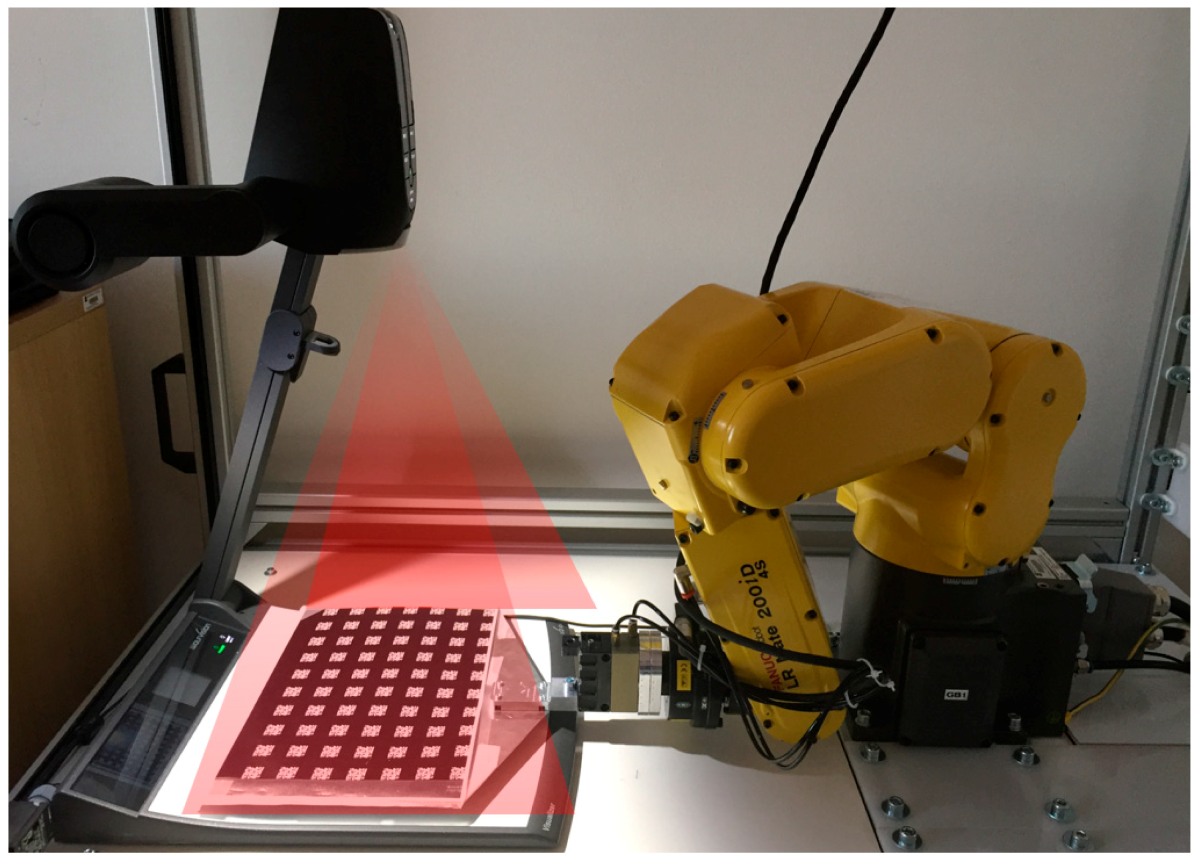
For this study, we used several hardware and software components that are described in the following subsections. Figure 1 shows the setup at the robot’s most frequent position (as close to the working surface as possible).
2.1. Robot
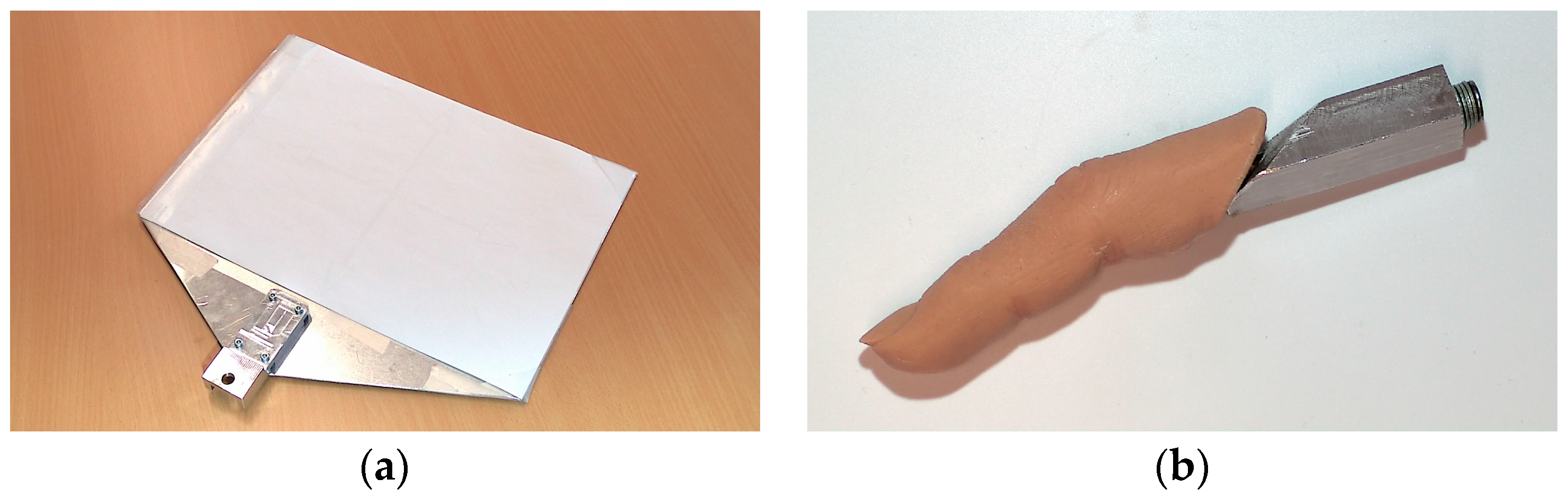
The robot that was used in our experiment was a FANUC LR Mate 200iD/4S (FANUC CORPORATION, Oshino, Japan). It had a repeatability of ±0.01 mm which we deemed sufficient, as the working area for maximum zoom was 32 by 18 mm2. It had 6 degrees of freedom and a spherical working envelope of 880 mm at the end effector. Due to the size of the product and the test patterns, we reached the limits of the robot’s range. The robot moved at a programmed speed of 4000 mm/s. The movements were of a linear type and ended at a stop point. The program running on the robot consisted of two parts: the commands to execute the desired movements, and several wait-functions which were used to start the movements at the right time. For most of the tests, we replaced the usual fingers of the gripper with a piece of aluminum sheet which was slightly larger than a standard A4-sized sheet of paper (see Figure 2a). We also added clear plastic parts to it, which were used to fix the patterns to the plate and enabled us to quickly change to the desired pattern. Another tool was an artificial silicone-finger, seen in Figure 2b, and a conventional ball pen.
The camera in the system recorded at 60 fps and had a natural resolution of 1920 by 1080 pixels. It had a maximum zoom factor of 14 times. It was mounted inside the head of the product, facing downwards, as seen in Figure 1 on the left side.
2.2. Scenarios
We gathered data from 7 patterns, 3 zoom levels, and 14 movements, creating 294 different scenarios. They are presented in the order shown below.
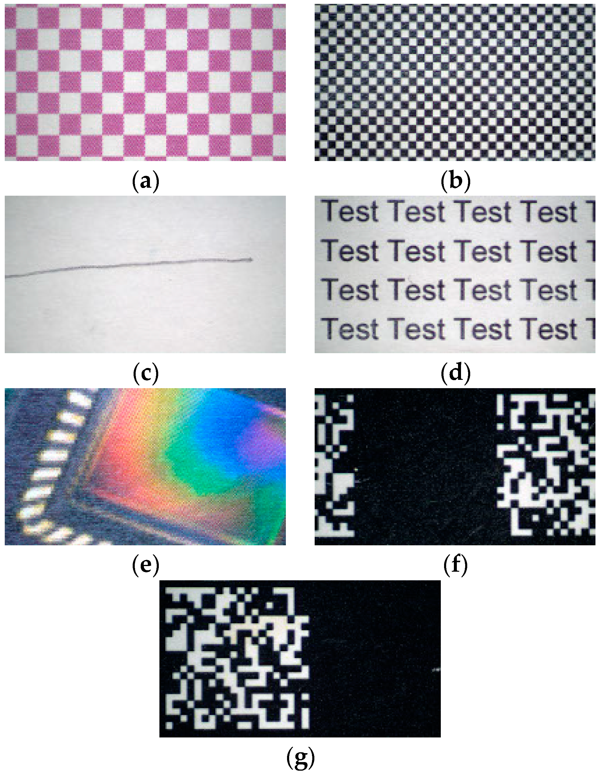
We printed the patterns on A4-sized sheets of paper and attached them to the robot. The patterns were chosen to cover high, low, and medium contrast as well as common situations like drawing on the working surface or showing text and colored images. Followed are short descriptions of the patterns:
- Checkered red: this checkered pattern filled almost the entire sheet; the squares were white and red. The size of a single square was 4 mm2. It had a medium contrast and resolution and was evenly distributed. See Figure 3a.
- Checkered black: the printed area was slightly larger than A5; it was black and white checkered with squares sized 0.64 mm2. It had a high contrast and small resolution and was evenly distributed. See Figure 3b.
- Pencil line: a single hand-drawn line, about 25 mm long. It had a low contrast and covered the use case of an end-user drawing on the working surface. See Figure 3c.
- Text: the word “Test” was printed all over a sheet (Arial, 8 pts). It covered the use case of showing a printed text. See Figure 3d.
- Graphics: a collection of various colorful pictures. It had high variability in contrast, resolution, and distribution. See Figure 3e.
- Dark pattern: a mostly black piece of paper with 70 matrix codes, each consisting of 40 0.49 mm2 sized cells. It had a very high contrast, variable resolution, and was unevenly distributed. See Figure 3f.
- Dark pattern rotated: as the pattern was asymmetric, we also tested it in a 180° rotated position. See Figure 3g.
We conducted the tests at three different zoom-levels:
- Maximum zoom (‘tele’): the zoom level where most details could be seen. On the working surface, this was an area of 2.8 by 1.5 mm2.
- Minimum zoom (‘wide’): the zoom level where most of the environment could be seen. On the working surface, this was an area of 390 by 220 mm2.
- A5: we defined this to be in between ‘tele’ and ‘wide’ as it was a very common setting for the system when an A4-sized sheet of paper was placed in a horizontal orientation. On the working surface, this was an area of 210 by 118 mm2.
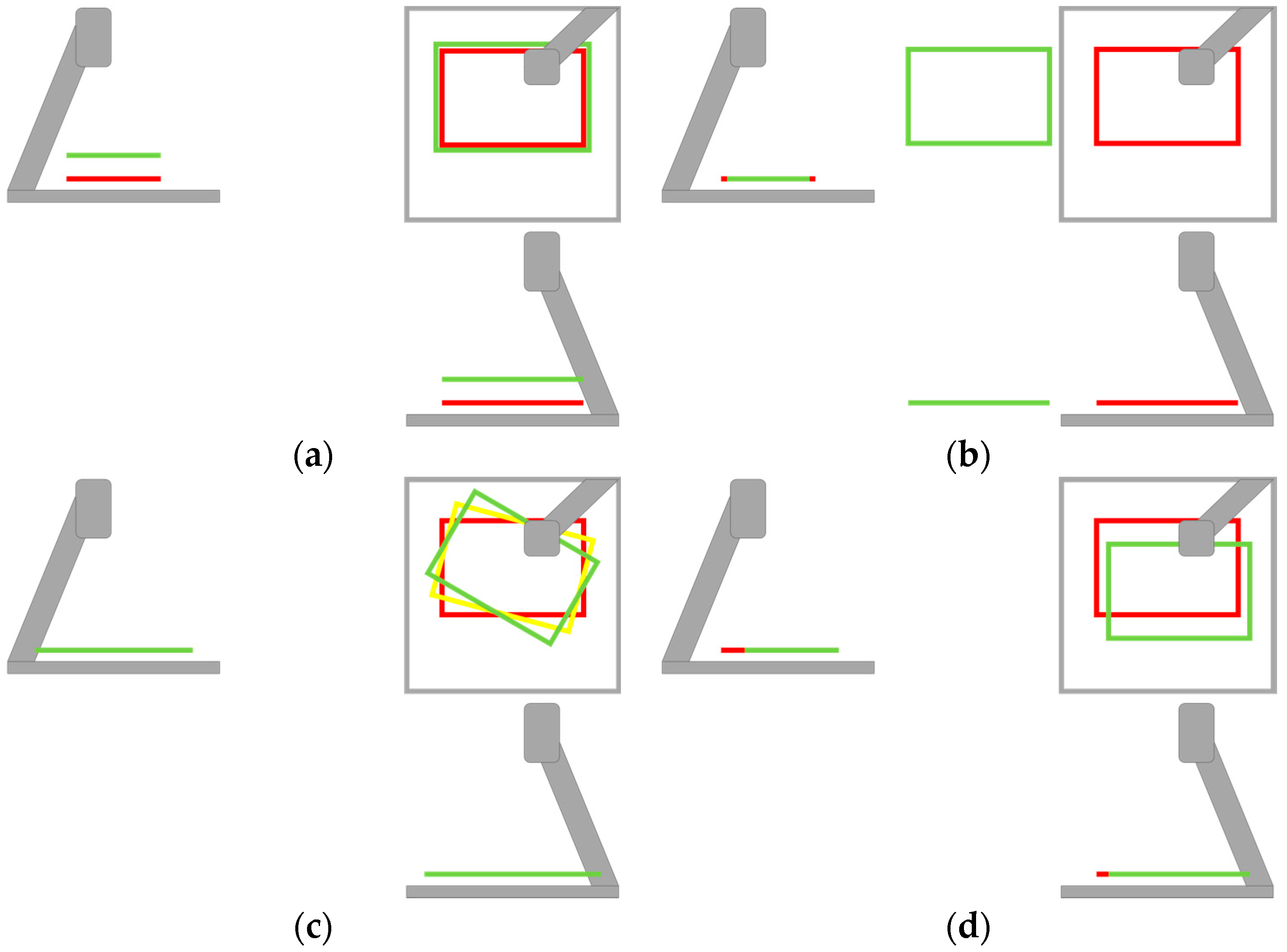
For a better understanding, the movements are depicted schematically in Figure A1 in Appendix A. They represented almost all possible movements that might occur during any presentation (for instance, moving the hand or a pointer, changing slides, moving a slide towards the optic, or putting a 3D element on the working surface). A time-lapse recording (Video S1) shows some of the movements. The movements were divided into three groups:
- The first one consisted of movements that happened while there was a fixed white background onto which the camera focused when it failed to find a focus position on the presented image. As the distance between the camera and surface was known, this focus was achieved with a fixed value:
- For the second movement group, we placed the patters onto the white background and mounted conventional grippers. Depending on the zoom level, we gripped a silicone finger (for A5 & wide zoom, see Figure 1b and Figure A1g) or a pen (for tele zoom, see Figure A1h). The respective tool moved from outside the robot’s field of view to the first position, stopped there, and moved again to the second position, stopped again, and then left the robot’s field of view. In these cases, the autofocus was not supposed to trigger. This covered the use-cases of pointing at the slide.
- The last category contained only one movement. We fixed a second layer (seen as the grey position in Figure A1i) showing some default text on top of the white background and repeated the ‘in’ movement at an increased height (from the green position in Figure A1i to the red position in Figure A1i). This covered the use-case of presenting a 3D-object.
2.3. Data Acquisition
A complete dataset with 10 loops in each scenario meant 2940 cycles, which took several hours to complete. In the end, we produced a table containing the arithmetic mean, median, maximum, minimum, and standard deviation for total focus time (the time between triggering the algorithm and its end) and final lens position, as well as the amount of timeouts (loops where the autofocus did not trigger at all). Two sets of data were generated between which the parameters of the autofocus algorithm were adapted. Gathering all of the data took a lot of time. For one measurement, the robot spent roughly 8 h waiting for the camera to find the focus or running into a timeout. Including other external factors (for instance, changing the pattern, getting the cell ready, or simply working for other projects), finishing one measurement took almost a week. Between the end of the first measurement and the beginning of the second, six more weeks passed (partially due to the holiday season).
2.4. Communication
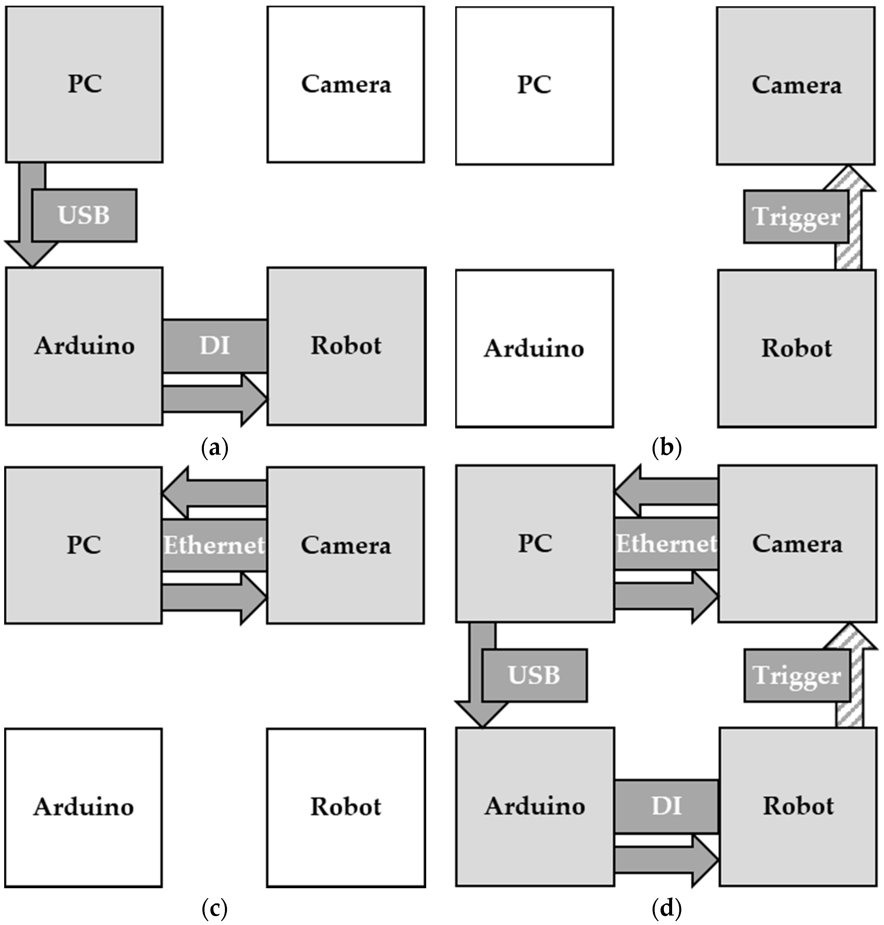
The setup had three independent but synchronized machines: camera, robot, and computer. The link between the camera and the PC was established via Ethernet and a respective TCP/IP protocol, which included a function to send the current lens position to the PC (see Figure 4c,d). The program on the computer compared these values to the previous one and continued requesting new positions until a certain timespan had passed. This was necessary to ensure that the focus had actually settled and would not shift again (see Figure 4c). The PC and robot were synchronized with an Arduino board: the PC sent the appropriate command whenever a certain state was reached via USB to the microcontroller, where two relay contacts were set accordingly. These were connected to two digital inputs (DI) at the robot controller. The robot program waited for the correct combination of these inputs. Depending on the state of the program, this could mean the confirmation of a found focus-position or the start of the program (see Figure 4a,d).
2.5. Adaptable Autofocus Parameters
The firmware of the camera had two adjustable groups of variables concerning the autofocus: sharpness and timing. The initial values were obtained by previously conducted manual tests and were therefore, as described in Section 1, a result of subjective impressions of the testing personnel.
The sharpness parameters, which were adapted in between the measurements, were:
- Sharpness minimum value to trigger the autofocus—a higher threshold leads to fewer triggers but could lead to cases where the image is out of focus.
- Sharpness variation margins to trigger the autofocus—connected to the first time constraint, this helps to reduce unwanted triggers by moving objects in the field of view.
- Sharpness margins between autofocus fields to decide where the object of interest is located—by segmenting the image—for instance a 3 by 3 matrix—and the importance of each field—for instance, a higher weight of the value from the center of the image in the “wide” zoom state.
There were also time constraints which influenced the algorithm gravely. The adapted parameters were:
- Averaging time to get rid of spurious peaks and undesired triggers due to hands and pointers or pens in the image
- Algorithm processing time limitation to reduce the probability of getting new sharpness values while dealing with the previous ones (e.g., to compensate for motor speed)
Due to the intellectual property of the algorithm itself and it not being the focus of this paper, we will not go into further detail and cannot publish exact values for the respective parameters (see the Supplementary Materials).
3. Results
Generally, we categorized the possible outcomes into three groups for each scenario: the autofocus triggered on each loop, never, or sometimes. The last cases were the most critical ones, as the algorithm did not perform consistently, meaning that the provided data had to be used to improve the system. If it neither was supposed to trigger nor did so, no changes had to be implemented. If the action of the algorithm was supposed to trigger and always did so, the presented data was going to be used to adjust the algorithm for speed.
After analyzing data from the first measurement, the results from the distinctive scenarios led to our proposed changes. The following adjustments were made to the parameters that were presented in Section 2.5:
- The sharpness minimum value to trigger the autofocus was reduced, as the various daily use cases were defined more clearly which predictably created a better focus result for small objects. This change stemmed from analyzing the average time and timeouts of the motive-moving scenarios over all zoom levels.
- The sharpness margins were increased, hoping to avoid excessive refocusing. The data backing this proposal were the average times of the laterally moving scenarios at tele zoom, where the times were surprisingly high.
- The margins between the fields were reduced which should help in finding small objects moving from one field to another while at tele zoom without compromising the performance at wide zoom. This was implemented due to the pen-scenarios at tele zoom.
- The averaging time was increased in tele and was reduced when going into a wide angle. This should decrease unwanted triggers by moving objects. The performance of the algorithm during the pen and finger scenarios allowed for this adaptation.
- The processing time was reduced in all cases, which should improve the algorithm’s precision. This was an update which should improve the results across all scenarios.
After this, a second dataset was generated and compared to the previous results. Table 1 on the next page shows the critical values for our evaluation. The meaning of the respective values is described below:
- The standard deviation of the average time it took the camera to find its focus was calculated for each of the 294 tested scenarios. The standard deviation total was the sum over all of the scenarios and was measured in milliseconds. It depicted the variation of each scenario’s average focus time. A decrease in this sum meant a more consistent behavior overall.
- Bad timeout scenarios were scenarios where the autofocus triggered between 1 and 9 times. This meant inconsistent behavior of the camera. An explanatory example: if 7 out of 10 loops were timeouts, we defined it as a bad timeout scenario and this value increased by 1. A decrease in this also meant that consistency had increased. The optimal value would be 0; the worst-case value was 294.
- The bad timeouts total was the sum of all runs which were part of an inconsistent 10-loop scenario. Similarly, the decrease of the bad timeouts total meant that the total probability of the occurrence of an inconsistent case decreased. An explanatory example: if 7 out of 10 loops were timeouts, this value increased by 7. The decrease was strongly linked to the previous value. Again, the optimal value would be 0 and the worst-case value would be 2646 (when the autofocus triggered 9 out of 10 times for each of the 294 scenarios).
- The average time measured the milliseconds it took the system to find its focus. The average time total was the sum over all of the scenarios and was measured in milliseconds. A lower value meant a faster algorithm.
4. Discussion
The first of the “8 golden rules” of Shneiderman, Plaisant, Cohen, Jacobs, Elmqvist, and Diakopoulos [2] is to “strive for consistency”. Comparing data from the first and second measurements shows that our system performed more consistently after the adaptations to the algorithm than before. This could be seen in the favorable decrease in the total standard deviation, which means that the average time to find the focus was more consistent (see row 1 in Table 1). The value for the bad timeout scenarios decreased, which means that the algorithm could better decide whether to trigger or not (see row 2 in Table 1). The value for the bad timeouts total (see row 3 in Table 1) decreased even more, which was connected to the previous value, but also meant that if a scenario was not well defined enough, it tended to not trigger at all. This second reason is also seen as favorable, as it aids in preventing a worst-case scenario, which is for the algorithm to trigger when the image is already in focus. In addition, as depicted in row 4 of Table 1, the adaptions led to slightly faster focus times on average. We are confident that further iterations and possible extensions of the testing will lead to an even more elaborated algorithm.
We believe that relying on objective real-world data is necessary to validate an algorithm like this. Relying on simulated images does not suffice, as they do not show the real use of the camera. If problems should arise in the daily use, we will create additional scenarios and adapt the benchmark for the parameters accordingly.
We are confident that this method is an improvement to the conventional methods of assessing an autofocus algorithm’s ability to work in the desired scenarios, as it shows exactly for which use-cases weaknesses exist, and what the results of a tweaked parameter mean for other cases. The proposed test could be applied to many different cameras and is not limited to the system that was used. Depending on the proposed field of use, the scenarios can be adapted freely.
To increase this even further, a lot of time and trial and error may be necessary, as the various thresholds need to be carefully fine-tuned to maximize the algorithm’s potential. We did not have the time to fully integrate the testing system, which in our case would necessitate the alteration of the firmware that is controlling the camera’s focal lenses. It should be noted that in our case, the time between the beginning of the first and second measurement was 7 weeks.
5. Conclusions
Validating and improving an autofocus algorithm is not an easy task when the images contain a lot of movement, as the input constantly changes and the system might not know how to react. Solutions from recent publications concerning autofocus problems with moving objects were not applicable in our situation, as a repetitive loop was necessary. We built a system which moved objectively and generated repeatable, non-biased data which developers could use to adapt their respective algorithm. The use-cases represented the standard day-to-day usage of the camera and could therefore be used to benchmark the algorithm. Comparing values from measurements before and after adjusting key parameters showed that the system had improved performance after just one loop. The behavior of the system was more consistent than before and therefore, led to higher usability and increased user experience for end-users.
We believe that this test could be run on any other type of autofocus algorithm, as it presented a variety of challenges to contrast and phase detection alike.
The next step is implementing a system that automatically finds the best parameters for the autofocus algorithm. This would drastically reduce the time of one iteration, possibly to a single week.
Supplementary Materials
The Video S1: Time-lapse movements is available online at https://www.mdpi.com/2218-6581/7/3/33/s1. To access the data generated by this study and further information concerning the materials and methods, please contact Tobias Werner. For information concerning the contrast detection algorithm, its parameters, and the influences of the data on it, please contact Javier Carrasco.
Author Contributions
T.W. and J.C. designed the experiments; T.W. programmed the robot and the interface, as well as performed the experiments; J.C. analyzed the data and adapted the algorithm parameters; T.W. wrote the paper.
Funding
Financial support for this project was provided by the Austrian research funding association (FFG) under the scope of the COMET program within the research project, “Easy to use professional business and system control applications (LiTech)” (contract # 843535).
Acknowledgments
This program is promoted by BMVIT, BMWFJ, and the federal state of Vorarlberg. Special thanks also to Andreas Wohlgenannt who helped us with the selection of patterns and movements, Alexander Brotzge for helping with the Ethernet-protocol, and to Walter Ritter who helped with synchronizing the PC and the robot.
Conflicts of Interest
The authors declare no conflict of interest. The founding sponsors had no role in the design of the study, in the collection, analyses, or interpretation of data, or in the writing of the manuscript and the decision to publish the results.
Appendix A
Figure A1.
The used movements in side, top, and front view: (a) up/down; (b) in/out; (c) rotation; (d) move; (e) 33% in; (f) 66% in; (g) finger; (h) pen; (i) layer; the red position in (a–d) is also seen in Figure 1.
Figure A1.
The used movements in side, top, and front view: (a) up/down; (b) in/out; (c) rotation; (d) move; (e) 33% in; (f) 66% in; (g) finger; (h) pen; (i) layer; the red position in (a–d) is also seen in Figure 1.


References
- Nakahara, N. Passive Autofocus System for a Camera. U.S. Patent 7,058,294, 6 June 2006. [Google Scholar]
- Shneiderman, B.; Plaisant, C.; Cohen, M.S.; Jacobs, S.; Elmqvist, N.; Diakopoulos, N. Designing the User Interface: Strategies for Effective Human-Computer Interaction; Pearson: New York, NY, USA, 2016. [Google Scholar]
- Mir, H.; Xu, P.; Chen, R.; Beek, P. An Autofocus Heuristic for Digital Cameras Based on Supervised Machine Learning. J. Heurist. 2015, 21, 599–616. [Google Scholar] [CrossRef]
- Chen, R.; van Beek, P. Improving the accuracy and low-light performance of contrast-based autofocus using supervised machine learning. Pattern Recognit. Lett. 2015, 56, 30–37. [Google Scholar] [CrossRef]
- Xu, X.; Wang, Y.; Zhang, X.; Li, S.; Liu, X.; Wang, X.; Tang, J. A comparison of contrast measurements in passive autofocus systems for low contrast images. Multimed. Tools Appl. 2014, 69, 139–156. [Google Scholar] [CrossRef]
- Bi, Z.; Pomalaza-Ráez, C.; Hershberger, D.; Dawson, J.; Lehman, A.; Yurek, J.; Ball, J. Automation of Electrical Cable Harnesses Testing. Robotics 2018, 7. [Google Scholar] [CrossRef]
- Shilston, R.T. Blur Perception: An Evaluation of Focus Measures. Ph.D. Thesis, University College London, London, UK, 2012. [Google Scholar]
- Dembélé, S.; Lehmann, O.; Medjaher, K.; Marturi, N.; Piat, N. Combining gradient ascent search and support vector machines for effective autofocus of a field emission–scanning electron microscope. J. Microsc. 2016, 264, 79–87. [Google Scholar] [CrossRef] [PubMed]
- Marturi, N.; Tamadazte, B.; Dembélé, S.; Piat, N. Visual Servoing-Based Depth-Estimation Technique for Manipulation Inside SEM. IEEE Trans. Instrum. Meas. 2016, 65, 1847–1855. [Google Scholar] [CrossRef]
- Cui, L.; Marchand, E.; Haliyo, S.; Régnier, S. Three-dimensional visual tracking and pose estimation in Scanning Electron Microscopes. In Proceedings of the 2016 IEEE/RSJ International Conference on Intelligent Robots and Systems (IROS), Daejeon, Korea, 9–14 October 2016; pp. 5210–5215. [Google Scholar]
Figure 1.
The main components of the setup: the presentation system with a downward facing camera, its field of view (symbolized by the transparent, red triangles), and the robot holding the dark pattern (see Section 2.2).
Figure 1.
The main components of the setup: the presentation system with a downward facing camera, its field of view (symbolized by the transparent, red triangles), and the robot holding the dark pattern (see Section 2.2).

Figure 2.
Robot-mounted hardware: (a) shows the fixture that was used to hold the patterns depicted in the next section (b) shows the finger that was used to move across the stationary patterns.
Figure 2.
Robot-mounted hardware: (a) shows the fixture that was used to hold the patterns depicted in the next section (b) shows the finger that was used to move across the stationary patterns.

Figure 3.
Various patterns at tele zoom: (a) checkered red; (b) checkered black; (c) pencil line; (d) text; (e) graphics; (f) dark pattern; (g) dark pattern flipped.
Figure 3.
Various patterns at tele zoom: (a) checkered red; (b) checkered black; (c) pencil line; (d) text; (e) graphics; (f) dark pattern; (g) dark pattern flipped.

Figure 4.
Schematic of the various steps of the synchronization (a) the PC signals the robot via an Arduino board to start (b) movement of the robot triggers the autofocus algorithm (c) the PC compares the focus values until they settle again (d) overview of all of the connections.
Figure 4.
Schematic of the various steps of the synchronization (a) the PC signals the robot via an Arduino board to start (b) movement of the robot triggers the autofocus algorithm (c) the PC compares the focus values until they settle again (d) overview of all of the connections.


Table 1.
Data showing the improvement of the algorithm.
| Measurement 1 | Measurement 2 | Difference | % | |
|---|---|---|---|---|
| Standard deviation total (ms) | 68,104.00 | 49,846.39 | 18,257.61 | −26.8 |
| Bad timeout scenarios (1) | 32 | 27 | 5 | −15.6 |
| Bad timeouts total (1) | 170 | 114 | 56 | −33.0 |
| Average time total (ms) | 631,767.92 | 601,232.02 | 30,535.90 | −4.8 |
© 2018 by the authors. Licensee MDPI, Basel, Switzerland. This article is an open access article distributed under the terms and conditions of the Creative Commons Attribution (CC BY) license (http://creativecommons.org/licenses/by/4.0/).
Share and Cite
MDPI and ACS Style
Werner, T.; Carrasco, J. Validating Autofocus Algorithms with Automated Tests. Robotics 2018, 7, 33. https://doi.org/10.3390/robotics7030033
AMA Style
Werner T, Carrasco J. Validating Autofocus Algorithms with Automated Tests. Robotics. 2018; 7(3):33. https://doi.org/10.3390/robotics7030033
Chicago/Turabian StyleWerner, Tobias, and Javier Carrasco. 2018. "Validating Autofocus Algorithms with Automated Tests" Robotics 7, no. 3: 33. https://doi.org/10.3390/robotics7030033
Note that from the first issue of 2016, this journal uses article numbers instead of page numbers. See further details here.