Calibration of UR10 Robot Controller through Simple Auto-Tuning Approach

Abstract

This paper presents a calibration approach of a manipulator robot controller using an auto-tuning technique. Since the industry requires machines to run with increasing speed and precision, an optimal controller is too demanding. Even though the robots make use of an internal controller, usually, this controller does not fulfill the user specification with respect to their applications. Therefore, in order to overcome the user requirements, an auto-tuning method based on a single sine test is employed to obtain the optimal parameters of the proportional–integral–derivative PID controller. This approach has been tested, validated and implemented on a UR10 robot. The experimental results revealed that the performances of the robot increased when the designed controller, using the auto-tuning technique, was employed.

1. Introduction

Manipulator robots can be described as automated electromechanical systems with flexible functionalities (i.e., programming according to the environmental conditions in which they operate). The main role of the manipulator robot is to help the human operators in fulfilling repetitive tasks with increased risk in an industrial environment. From the perspective of robot control, focus is put on the structure and functionality of the robot command unit. Based on the dynamic and geometrical model and the tasks that need to be performed, appropriate commands are established. In order to provide these commands to the actuators, the hardware and the software, it is required to use the feedback signals obtained from the sensory system unit [1]. Due to the complexity of the manipulator robot, the control architecture has a hierarchical structure. The upper level makes the decision with respect to the actions that need to be taken (e.g., simple test based on “if-then” actions), while the lower level carries out the control of the joints. The typical structure of the control system consists of a computer on the upper level and a system with one or more microcontrollers to drive the actuators of the joints on the lower level.

Mechatronic systems, in special robots, are very popular for control applications due to their interdisciplinary nature [2,3,4]. For linear mechatronic systems, the proportional-integral-derivative (PID) controller has been widely used given its simple structure and robustness [5]. Usually, the design of conventional integer-order PID controllers is based on the model of the system.

The manipulator robots are also used in medicine for precision surgery [6,7,8]. Surgery has become an extremely precise practice, and professionals often have to make movements in the order of hundreds of microns. The inherent limits of human dexterity are a constraint for new advances in this field. In this context, high-precision robotics are being developed and implemented for medical use [9,10]. From the observation of these devices, it is possible to acquire an idea of their versatility. Not only in medicine, but in the high-tech industry, as well, robotic automation is highly competitive and requires very high precision and better performance. Therefore, the performance specifications of control have also become extremely demanding.

In these real applications of the UR10 robot, the characteristics of the system may be subject to changes (e.g., the mass attached to the end effector, the speed of the joints (TCP respectively), the required precision, etc.). The controller, however, has to keep its performance constantly optimal. Usually, the robots already have an internal control loop, making the robot stable and performing quite well. Nevertheless, this controller cannot fulfill all the user specifications and does not perform optimally in all situations. Therefore, a new controller is employed in order to overcome the user requirements [11,12,13,14]. Hitherto, PID control is widely used in control engineering and industry. The most challenging step in employing PID controllers, for non-experts in control engineering, is the process of parameter tuning. Nowadays, the self-tuning PID digital controller provides much convenience in engineering [15,16]. Optimal control of a plant (in this particular application, the robot arm) is highly dependent on the plant behavior.

Throughout the years, several methods have been introduced [17,18,19] to improve the tuning principles proposed by Ziegler and Nichols. Astrom and Hagglund proposed an AMIGO (approximate M-constrained integral gain optimization) tuning rule for PI controllers [20], based on the ideas presented in [21], where the tuning of the controllers is done so as to maximize the integral gain subject to constraints on the maximum sensitivity. The same approach was later extended to PID controllers [22] and finally perfected by adding additional constraints [23] to make the tuning method suitable for a wide class of processes. Skogestad proposed a novel tuning rule based on the ideas behind IMC (internal model control) that have achieved widespread industrial acceptance [24]. These novel tuning rules, referred to as SIMC (Skogestad IMC), work well for both integrating and pure time delay processes, for both setpoint changes and load disturbances and are suitable for first-order or second-order time delay models.

In this paper, we propose simple and efficient calibration of the robot controller based on an auto-tuning procedure. The auto-tuning method attempts to design PID controllers that ensure a minimum phase margin PM = 45° and a minimum gain margin GM = 2. The method is based on defining a forbidden region in the Nyquist plane, using the performance specifications, and then searches for the optimal PID controller that ensures that the difference between the slope of the region border and the loop frequency response slope is minimum. This requirement leads to PID controllers that are robust to gain, as well as to phase and delay variations. Although the method has already been compared to various other popular PID tuning methods [25], its main features have not been fully revealed. To design the PID controller, a single sine test is applied to the robot to determine its frequency response and its frequency response slope [26], needed in the auto-tuning procedure. The original elements of this paper include, apart from a detailed description of the auto-tuning method, also the particularities of using it in a closed loop setting. Moreover, for the first time, the auto-tuning method is validated experimentally.

This paper is structured as follows: The next section gives a description of the robotic system used in this study. Section 3 discusses the automatic calibration of the robot using an auto-tuning approach. Section 4 presents the implementation and the corresponding results of the tuning procedure. The conclusion is formed in Section 5.

2. System Description

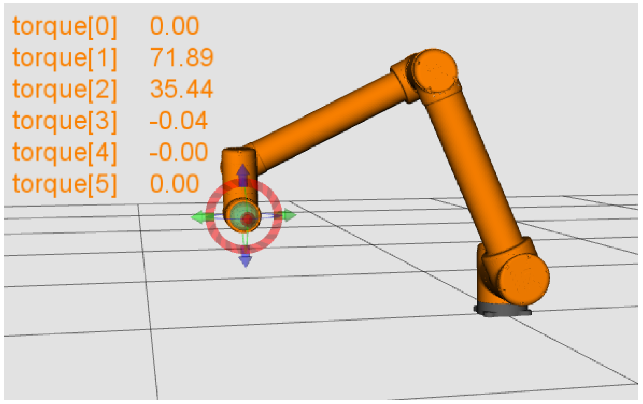
A robot manipulator, depicted in Figure 1, can be defined as a kinematic chain consisting of multiple rigid bodies, which are interconnected by joints. Every joint of the kinematic chain consists of one degree of freedom, which can be translational or rotational. In the work of Spong et al. [1], it is mentioned that a simple representation of a robot manipulator joint can be modeled as a spring with linear constant stiffness. Based on the Lagrangian formulation, the dynamics of a global manipulator robot with n revolute joints are given by [27]:

$$Q=M\left(q\right)\ddot{q}+C(q,\dot{q})\dot{q}+F\left(\dot{q}\right)+G\left(q\right)+J{\left(q\right)}^T\eta$$

(1)

where $q,\dot{q},\ddot{q}\in {\Re }^n$ represent the joint variables (the generalized joint coordinates, the velocity and the acceleration), $M\left(q\right)\in {\Re }^{n\times n}$ is the inertia matrix, $C(q,\dot{q})$ is the $n\times 1$ vector of the Coriolis and centrifugal forces, $F\left(\dot{q}\right)$ is the friction torque, $G\left(q\right)$ is the gravity force and Q is a vector representing the actuator forces associated with the joint coordinates q. The matrix $J{\left(q\right)}^T$ is the transpose of the Jacobian matrix of the robot, while $\eta$ is the joint force vector applied at the robot end-effector.

The matrices $M,C,F$ and G are composed of complex functions, which describe the kinematic link dynamics through a set of parameters (${\theta }_j,d_j,a_j,{\alpha }_j$), $j=1,\dots ,n$, also known as Denavit–Hartenberg parameters.

The considered UR10 robot studied in this paper has the following Denavit–Hartenberg (D-H) parameters; see

Table 1. Denavit–Hartenberg (D-H) parameters.

Joint	$\mathit{\theta }$	d	a	$\mathit{\alpha }$
1	${\theta }_1$	0.12	0	$pi/2$
2	${\theta }_2$	0	−0.61	0
3	${\theta }_3$	0	−0.57	0
4	${\theta }_4$	0.16	0	$pi/2$
5	${\theta }_5$	0.11	0	$-pi/2$
6	${\theta }_6$	0.09	0	0

.

The highest variation in the robot dynamics is introduced by the gravity matrix and the inertia matrix. The gravity term is present even when the robot is stationary or moving slowly. The torque exerted on a joint due to gravity acting on the robot is strongly dependent on the position and orientation of the robot.

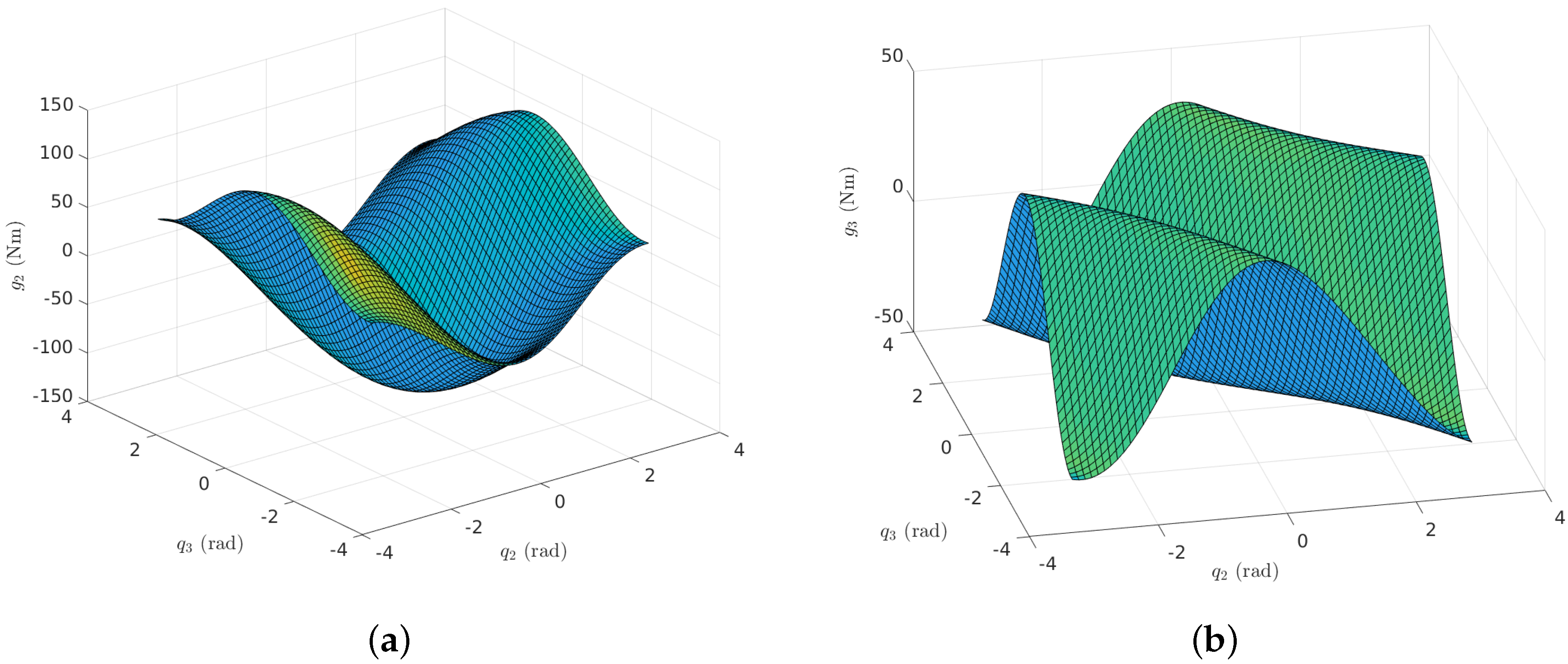
Due to the construction of the robot (three large joints and three small joints), we expect to have a larger variation introduced by the shoulder joint and elbow joint. For example, the gravity torque acting on the elbow joint is higher when the robot is in a position such that the elbow joint has to support the shoulder-lift joint and the wrist joint. To illustrate this aspect, we have investigated the variation of the gravity load for Joint 2 (shoulder-lift joint) and Joint 3 (elbow joint) with respect to the robot configuration. The obtained results are illustrated in Figure 2. As observed, Joint 2 has a larger variation ($\pm 100$ Nm) compared to Joint 3 ($\pm 40$ Nm). This analysis is important for robot design, as well as for control design in order to ensure a feasible control input for the motors.

The gravity matrix is not the only term that varies with respect to the position of the robot. The other matrix that is highly dependent on the robot pose is the inertia matrix. By inspecting the elements of this matrix, we observe that it is symmetric with diagonal terms $M_{jj}$ describing the inertia related to joint j. The other elements $M_{ji}$ of the inertia matrix represent the coupling between joint j and joint i. In Figure 3, we can see the variation of the Joint 1 inertia with respect to the pose of the robot (here, Joint 2 and Joint 3 are varying between −180 and +180).

In most of the robotics applications, one needs to control the pose of the end-effector, which can be done through the direct kinematics formulation. In this research study, a six-degree of freedom manipulator robot is considered; thus, the direct kinematic equation is given as:

$${}^0{T}_6\left(q\right){=}^0{A}_1{\left(q_1\right)}^1{A}_2\left(q_2\right){\dots }^5{A}_6\left(q_6\right),$$

(2)

where ${}^{i-1}{A}_i\left(q_i\right),i=\overline{1,6}$ represent the homogeneous transformation matrices. The direct kinematics can be calculated via the Denavit–Hartenberg (D-H) formulation [28].

Starting from the assumption that the pose, the velocity and the acceleration are known and based on Equation (1), it is possible to calculate the required joint torques.

Given the pose configuration of the end-effector, the joint variables corresponding to this configuration can be calculated using the inverse kinematics formulation. The inverse kinematics is a very challenging problem since it is almost impossible to obtain a unique solution. In the literature, there are two approaches used to calculate the inverse kinematics: the analytical method and the numerical method [28]. Here, a numerical method was considered [27]. The existence of solutions is guaranteed only if the given end-effector position and orientation belong to the manipulator’s dexterous workspace.

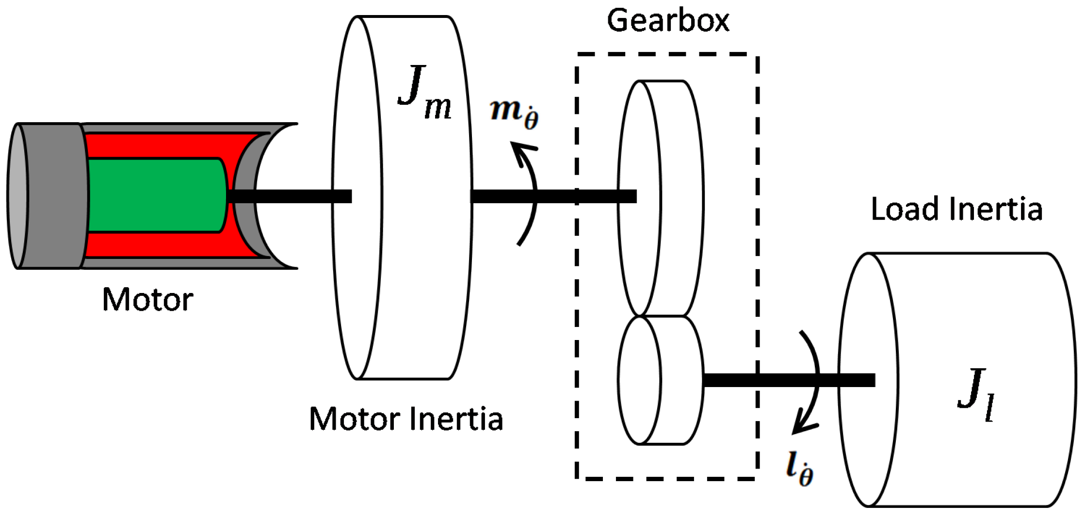
Nowadays, a large number of the industrial robots are driven by brushless servo motors. A schematic overview of a classical robot joint is illustrated in Figure 4.

Several studies in the area of the control of manipulator robots consider as control variables the Cartesian coordinates. However, in order to obtain the desired Cartesian trajectory for the end-effector attached to the robot, each joint axis must follow a specific trajectory. The common approach to control the robot joints is based on the decentralized techniques, which consider an independent controller for each joint. The industrial robot considered for our experiments is electrically actuated. If the robot joint drivetrain is driven by the current:

$$i=K_{a}u$$

(3)

then the torque generated by the motor is proportional to the current:

$$\tau =K_{m}i$$

(4)

where $K_a$ is the transconductance of the amplifier, $K_m$ is the motor torque constant and u is the applied control voltage. Based on this assumption, the dynamics of a motor attached to a joint j can be defined as:

$$J_m\dot{\omega }+B\omega +{\tau }_c\left(\omega \right)=K_m{K}_{a}u$$

(5)

with ${\tau }_c$ Coulomb’s law of friction, B the viscous friction and $J_m$ the total inertia seen by the motor for joint j, computed as:

$$J_m=J_{m_j}+\frac{1}{G_j^2}{M}_{jj}.$$

(6)

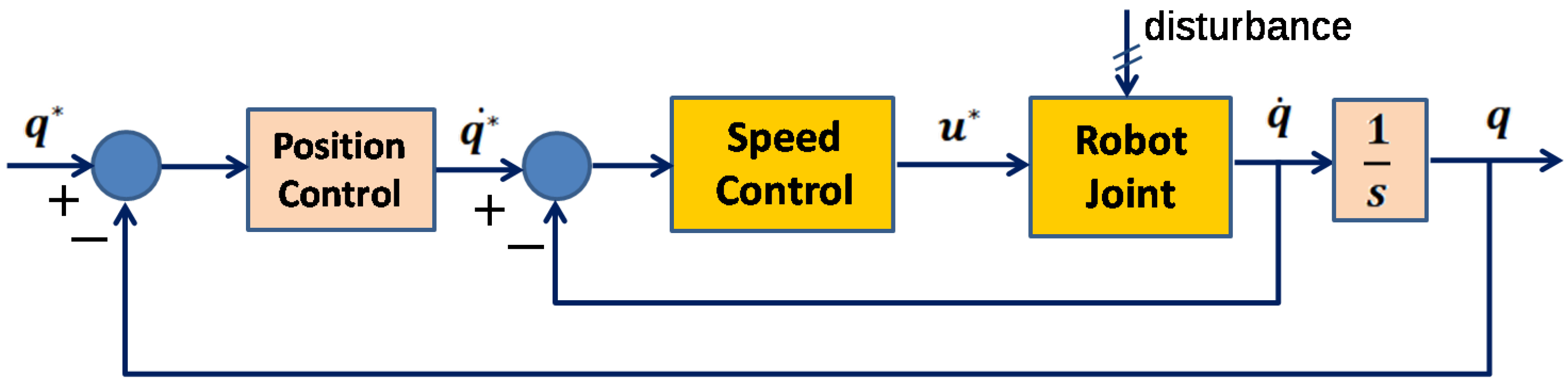
Since in real life, disturbance torques such as gravity and friction can act on the joints, the common approach where independent control systems are considered to control the robot joints is no longer efficient. The control performance decreases, leading to high overshoot and large steady-state error. A classical approach to overcome these shortcomings is to use a nested control structure composed of two loops: one outer loop and one inner loop, as depicted in Figure 5. The outer loop is used to control the position and to provide the velocity of the joints in order to minimize the position error, while the inner loop is used to minimize the error between the actual velocity of the joint and the velocity demanded by the outer loop.

For simplification purposes, if the Coulomb friction from Equation (5) is ignored, the equivalent Laplace transform of (5) is given by:

$$sJ\Omega \left(s\right)+B\Omega \left(s\right)=K_m{K}_{a}U\left(s\right)$$

(7)

where $\Omega \left(s\right)$ and $U\left(s\right)$ are the Laplace transform of their corresponding signal from time domain $\omega$ and u. Thus, the transfer function of a motor drivetrain attached to a robot joint can be written as:

$$\frac{\Omega \left(s\right)}{U\left(s\right)}=\frac{K_m{K}_a}{Js+B}.$$

(8)

Typically, a PI controller is used to drive the robot joint from the actual velocity to its demanded velocity. However, in this experiment, it is no need for good closed loop dynamics; therefore, a P controller has been selected (note that the P controller was used only for tests in order determine the process frequency response and process frequency response slope) for simplicity in the computations in the next section, and thus, we have:

$$u^{*}=K_p({\dot{q}}^{*}-\dot{q}).$$

(9)

3. Robust Control Design

3.1. A Robust Method to Estimate the Process Frequency Response

The frequency response of a process at a specific frequency $\overline{\omega }$ can be written as:

$$P\left(j\overline{\omega }\right)=\frac{A_y}{A_u}{e}^{j{\phi }_y}$$

(10)

where $A_y$ stands for the amplitude of the output signal $y\left(t\right)$, $A_u$ is the amplitude of the input signal $u\left(t\right)=A_{\omega }sin\left(\overline{\omega }t\right)$ and ${\phi }_y$ is the phase of the output signal $y\left(t\right)$. To determine experimentally the frequency response in (10), a robust procedure is needed to evaluate correctly, even in the presence of severe disturbances, the amplitude $A_y$ and phase ${\phi }_y$ of the output signal $y\left(t\right)$. Such a procedure is based on the transfer function analyzer-discrete Fourier transform (TFA-DFT) [29,30].

For the process with the frequency response given in (10), the steady-state response can be written as:

$$y\left(t\right)=A_{y}sin(\overline{\omega }t+{\phi }_y)+b+n\left(t\right)$$

(11)

where $n\left(t\right)$ is the stochastic disturbance with zero mean value and b is a non-zero bias term ($b\ne 0$ in the case of a nonzero average disturbance).

Consider the multiplication of the measured output $y\left(t\right)$ by sine and cosine functions of the frequency of the system input $\overline{\omega }$ and then integrated over the measurement period $T_m=k\frac{2\pi }{\overline{\omega }}$, with k an integer value [29,30]. Then, the following results are obtained:

$$y_s={\int }_0^{T_m}y\left(t\right)sin\left(\overline{\omega }t\right)dt=A_y{\int }_0^{T_m}\left(sin\left(\overline{\omega }t\right)cos{\phi }_y+cos\left(\overline{\omega }t\right)sin{\phi }_y\right)sin\left(\overline{\omega }t\right)dt+{\int }_0^{T_m}\left(b+n\left(t\right)\right)sin\left(\overline{\omega }t\right)dt$$

(12)

$$y_c={\int }_0^{T_m}y\left(t\right)cos\left(\overline{\omega }t\right)dt=A_y{\int }_0^{T_m}\left(sin\left(\overline{\omega }t\right)cos{\phi }_y+cos\left(\overline{\omega }t\right)sin{\phi }_y\right)cos\left(\overline{\omega }t\right)dt+{\int }_0^{T_m}\left(b+n\left(t\right)\right)cos\left(\overline{\omega }t\right)dt$$

(13)

An analysis of the right-hand side terms in (12) and (13) leads to a simplification, provided that there is an increase in the averaging time. In this case, the contribution of the last terms can be neglected compared to the first term, which is growing with $T_m$. Furthermore, it is assumed that for a long integration time, the noise $n\left(t\right)$ will be filtered out (i.e., zero average) [30]. In this case, (12) reduces to:

$$y_s=A_{y}cos{\phi }_y{\int }_0^{T_m}si{n}^2\left(\overline{\omega }t\right)dt+0.5A_{y}sin{\phi }_y{\int }_0^{T_m}2cos\left(\overline{\omega }t\right)sin\left(\overline{\omega }t\right)dt$$

(14)

The result in (14) is valid even in the case of low signal-to-noise ratios provided that $n\left(t\right)$ is a stochastic disturbance with zero mean value and a sufficient number of test signal periods is selected [29].

After some mathematical rearrangement of the terms in (14), the following result is obtained:

$$y_s=0.5T_m{A}_{y}cos{\phi }_y-0.5A_{y}cos{\phi }_y\frac{sin\left(2\overline{\omega }{T}_m\right)}{2\overline{\omega }}-0.5A_{y}sin{\phi }_y\frac{cos\left(2\overline{\omega }{T}_m\right)-1}{2\overline{\omega }}$$

(15)

Assuming that $T_m=k\frac{2\pi }{\overline{\omega }}$, as mentioned above, namely the measurement (also integration) time is an integer number of periods, the last two terms in (15) will be zero. Then, a simplified result for (12) is finally obtained as:

$$y_s=0.5T_m{A}_{y}cos{\phi }_y$$

(16)

A similar analysis can be performed for the signal in (13), leading to:

$$y_c=0.5T_m{A}_{y}sin{\phi }_y$$

(17)

Using (12) and (13) leads to:

$$y_c-j{y}_s={\int }_0^{T_m}y\left(t\right)\left(cos\left(\overline{\omega }t\right)-jsin\left(\overline{\omega }t\right)\right)dt={\int }_0^{T_m}y\left(t\right)e^{-j\overline{\omega }t}dt$$

(18)

The integral ${\int }_0^{T_m}y\left(t\right)e^{-j\overline{\omega }t}dt$ in (18) can be calculated via the DFT:

$${\int }_0^{T_m}y\left(t\right)e^{-j\overline{\omega }t}dt=T_s\sum _0^{N-1}y\left(k{T}_s\right)e^{-j\overline{\omega }k{T}_s}$$

(19)

where $T_s$ is the sampling period, chosen such that $T_m=N{T}_s$. Using now (16) and (17), the next result holds:

$$y_c-j{y}_s=-j0.5T_m{A}_y(cos{\phi }_y+jsin{\phi }_y)=-j0.5T_m{A}_y{e}^{j{\phi }_y}$$

(20)

which leads to:

$$A_y{e}^{j{\phi }_y}=\frac{y_c-j{y}_s}{-j0.5T_m}$$

(21)

Using (18) and (19) in (21) leads to:

$$A_y{e}^{j{\phi }_y}=\frac{T_s{\sum }_0^{N-1}y\left(k{T}_s\right)e^{-j\overline{\omega }k{T}_s}}{-j0.5T_m}$$

(22)

Taking into account that $T_m=N{T}_s$ and rearranging (22) leads to the following solution for determining robustly the amplitude $A_y$ and phase ${\phi }_y$ of the output signal $y\left(t\right)$ [26]:

$$A_y{e}^{j{\phi }_y}=\frac{2j}{N}\sum _0^{N-1}y\left(k{T}_s\right)e^{-j\overline{\omega }k{T}_s}$$

(23)

3.2. A Robust Method to Estimate the Process Frequency Response Slope

For the purpose of designing the PID controller using the KC auto-tuning method [26], the frequency response slope needs to be determined, as well. For the process $P\left(s\right)$, the frequency response slope is given as:

$${\left.\frac{dP\left(j\omega \right)}{d\omega }\right|}_{\omega =\overline{\omega }}=j\frac{A_{\overline{y}}}{A_u}{e}^{j{\phi }_{\overline{y}}}$$

(24)

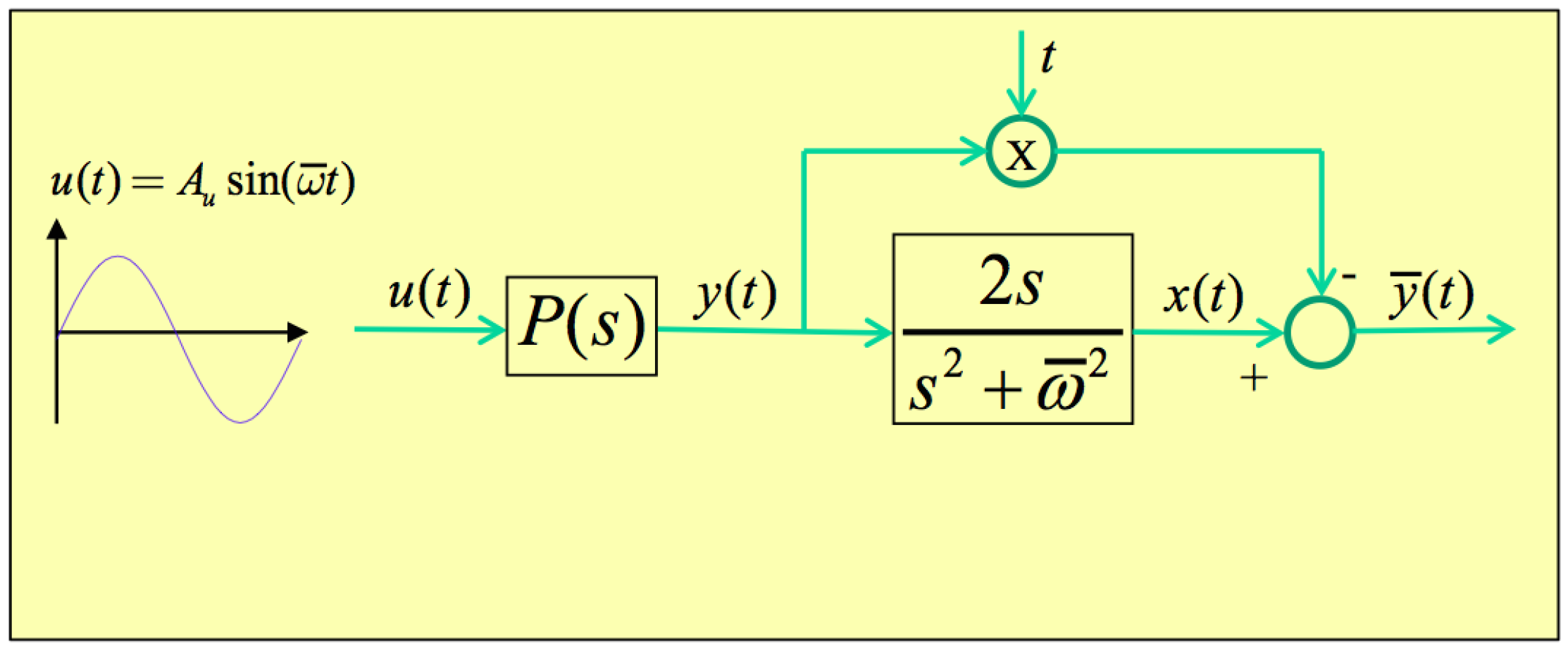
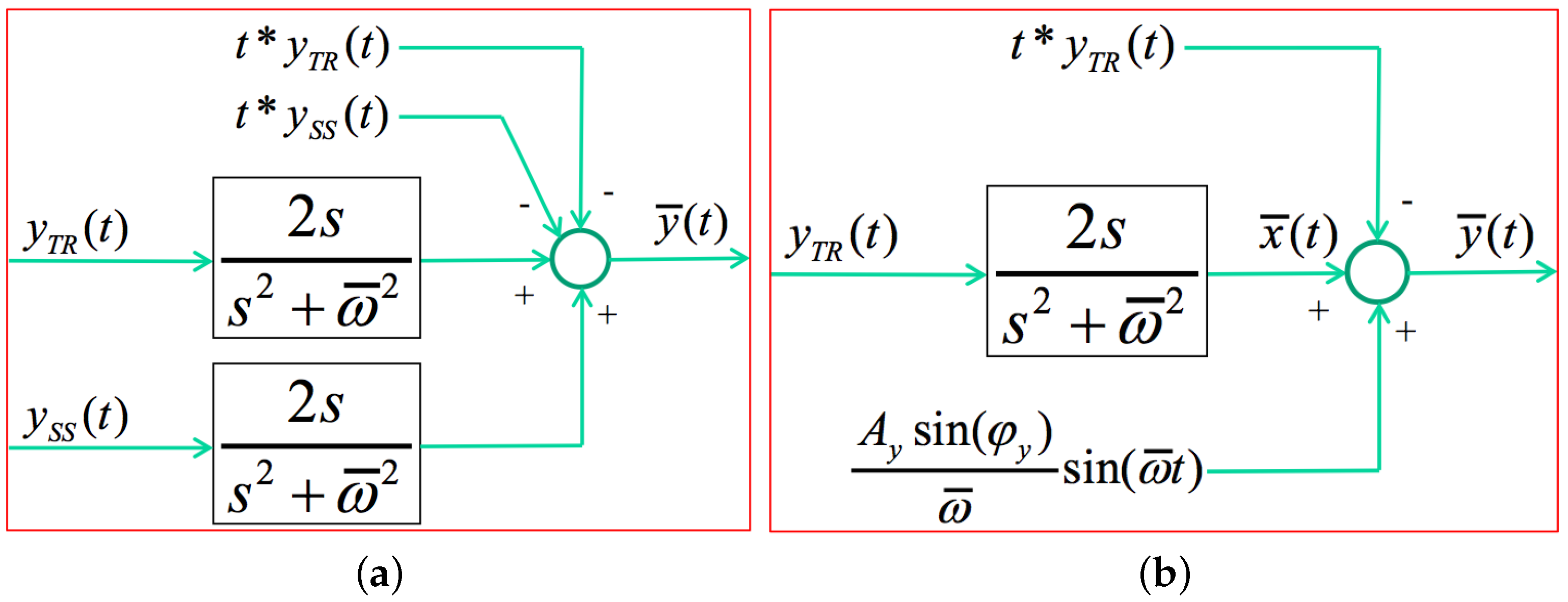
A simple strategy to estimate (24) has been developed previously, and it is based on filtering the output signal $y\left(t\right)$ as indicated in Figure 6 [31]. The strategy is simple, but prone to errors in the case of stochastic disturbances and noise [26]. An elegant solution to eliminate this problem has been developed and consists of a modification of the basic scheme in Figure 6 as indicated in Figure 7a, where $y_{TR}\left(t\right)$ and $y_{SS}\left(t\right)$ are the transient and steady-state parts of the output signal $y\left(t\right)$, with the transient component going to zero (or to a constant value for an integrating system) [26].

The steady-state component of the output signal can be written simply as:

$$y_{SS}\left(t\right)=A_{y}sin(\overline{\omega }t+{\phi }_y)=Ssin\left(\overline{\omega }t\right)+Ccos\left(\overline{\omega }t\right)$$

(25)

where $S=A_{y}cos\left({\phi }_y\right)$ and $C=A_{y}sin\left({\phi }_y\right)$. Applying the Laplace transform to (25) leads to:

$$Y_{SS}\left(s\right)=\frac{S\overline{\omega }}{s^2+{\overline{\omega }}^2}+\frac{Cs}{s^2+{\overline{\omega }}^2}=\frac{S\overline{\omega }+Cs}{s^2+{\overline{\omega }}^2}$$

(26)

Applying the derivative to (26) leads to the following:

$$\begin{array}{c}\frac{d{Y}_{SS}\left(s\right)}{ds}=\frac{C(s^2+{\overline{\omega }}^2)-2s(S\overline{\omega }+Cs)}{{(s^2+{\overline{\omega }}^2)}^2}=\frac{C}{(s^2+{\overline{\omega }}^2)}-\frac{2s}{(s^2+{\overline{\omega }}^2)}\frac{S\overline{\omega }+Cs}{(s^2+{\overline{\omega }}^2)}=\frac{C}{(s^2+{\overline{\omega }}^2)}-\frac{2s}{(s^2+{\overline{\omega }}^2)}{Y}_{SS}\left(s\right)\hfill \end{array}$$

(27)

The following result is obtained using the inverse Laplace transform on (27):

$$-t{y}_{SS}\left(t\right)=\frac{A_{y}sin\left({\phi }_y\right)}{\overline{\omega }}sin\left(\overline{\omega }t\right)-{\mathfrak{L}}^1\left(\frac{2s}{s^2+{\overline{\omega }}^2}{Y}_{SS}\left(s\right)\right)$$

(28)

Figure 7a can now be replaced by Figure 7b, using the result in (28). The Laplace transform of the signal $x\left(t\right)$, computed based on Figure 7b, is obtained as:

$$\overline{X}\left(s\right)=\frac{2s}{s^2+{\overline{\omega }}^2}{Y}_{TR}\left(s\right)=\frac{2s}{\overline{\omega }}{Y}_{TR}\left(s\right)\frac{\overline{\omega }}{s^2+{\overline{\omega }}^2}$$

(29)

Applying the inverse Laplace transform to (29) and considering that $\frac{\overline{\omega }}{s^2+{\overline{\omega }}^2}={\mathfrak{L}}^{-1}sin\left(\overline{\omega }t\right)$ leads to:

$$\overline{x}\left(t\right)={\mathfrak{L}}^{-1}\{\frac{2s}{\overline{\omega }}{Y}_{TR}\left(s\right)\}sin\left(\overline{\omega }t\right)$$

(30)

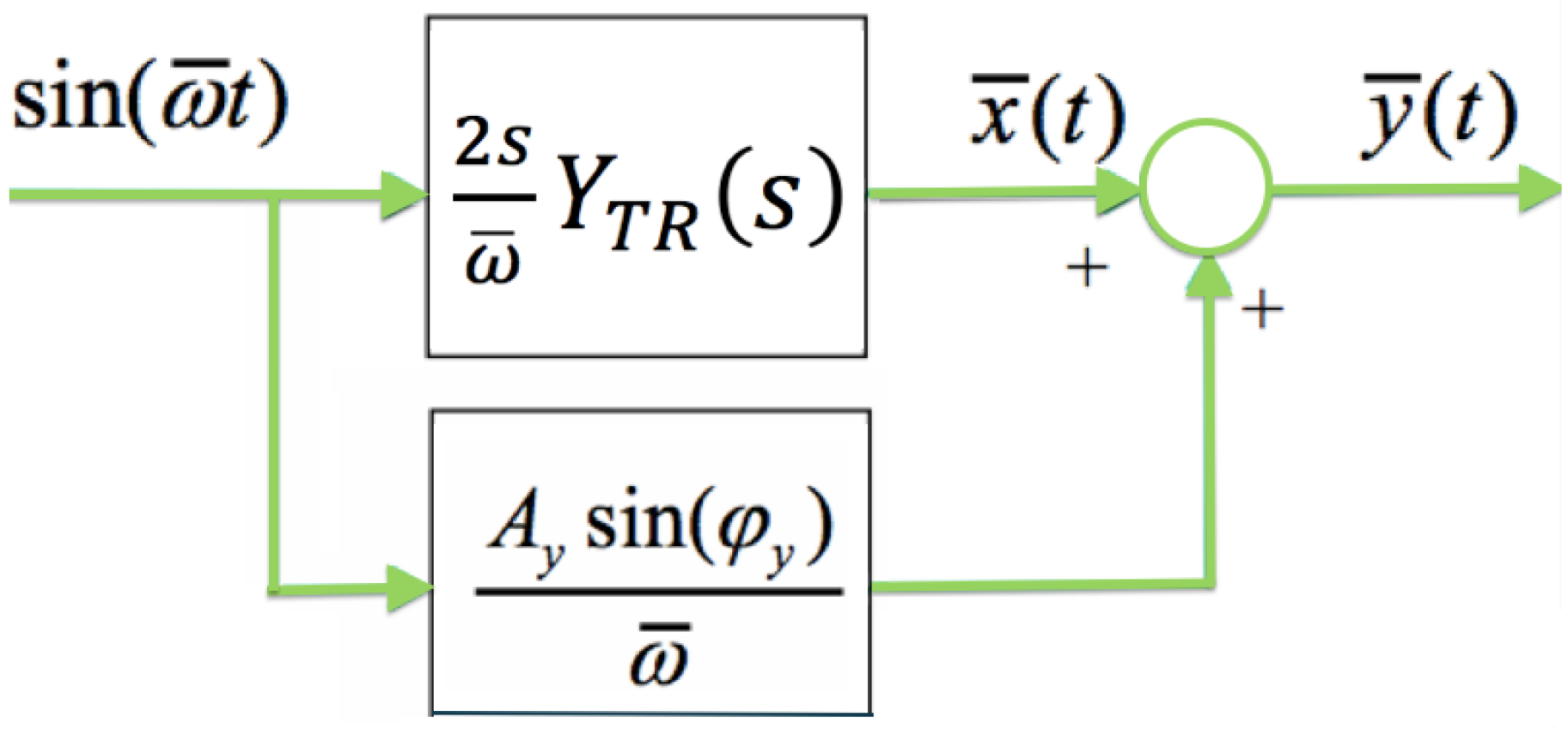
However, the component $t*y_{TR}\left(t\right)$ does not influence the steady-state oscillation in $\overline{y}\left(t\right)$ and the result in (30). In this case, Figure 7b reduces to the simplified version in Figure 8.

Using the result in Figure 8 leads to a means of computing the amplitude $A_{\overline{y}}$ and phase ${\phi }_{\overline{y}}$ of the signal $\overline{y}\left(t\right)$ at the specific frequency $\overline{\omega }$ as:

$$A_{\overline{y}}{e}^{j{\phi }_{\overline{y}}}=A_{\overline{x}}{e}^{j{\phi }_{\overline{x}}}+\frac{A_{y}sin\left({\phi }_y\right)}{\overline{\omega }}$$

(31)

Since the test frequency $\overline{\omega }$ is user specified and the amplitude $A_y$ and phase ${\phi }_y$ of the output signal $y\left(t\right)$ are determined as mentioned previously, in order to determine the amplitude $A_{\overline{y}}$ and phase ${\phi }_{\overline{y}}$, the corresponding amplitude $A_{\overline{x}}$ and phase ${\phi }_{\overline{x}}$ have to be computed, as well. These can be obtained from the frequency response of the system $\frac{2s}{\overline{\omega }}{Y}_{TR}\left(s\right)$, as indicated in Figure 8. Using the definition of the Laplace transform, the following relation is valid:

$$\frac{2s}{\overline{\omega }}{Y}_{TR}\left(s\right)=\frac{2s}{\overline{\omega }}{\int }_0^{\infty }{y}_{TR}\left(t\right)e^{-st}dt$$

(32)

Then, the amplitude $A_{\overline{x}}$ and phase ${\phi }_{\overline{x}}$ are computed according to:

$$A_{\overline{x}}{e}^{j{\phi }_{\overline{x}}}=2j{\int }_0^{\infty }{y}_{TR}\left(t\right)e^{-j\overline{\omega }t}dt$$

(33)

where the discrete Fourier transform is used to evaluate the integral on the right-hand side of (33) as:

$${\int }_0^{\infty }{y}_{TR}\left(t\right)e^{-j\overline{\omega }t}dt=T_s\sum _{k=0}^{N-1}{y}_{TR}\left(k{T}_s\right)e^{-j\overline{\omega }k{T}_s}$$

(34)

3.3. The Closed Loop Implementation

The robust procedures in the previous sections assume that an input signal can be applied to the process. In case the loop cannot be opened to enter a test-sine in the process $P\left(s\right)$, a closed loop approach must be considered. For this purpose, a test-sine $w\left(t\right)=A_{w}sin\left(\overline{\omega }t\right)$ must be used, where $w\left(t\right)$ is the reference signal of the closed loop system. Figure 9 illustrates this approach. The output $y\left(t\right)$ is measured, and the error signal $e\left(t\right)$ is further computed as $e\left(t\right)=w\left(t\right)-y\left(t\right)$. Applying the procedure described in Section 3.1 and Section 3.2 to the signals $w\left(t\right)$ and $e\left(t\right)$ leads to the frequency response $S\left(j\overline{\omega }\right)$ and the frequency response slope ${\left.\frac{dS\left(j\omega \right)}{d\omega }\right|}_{\omega =\overline{\omega }}$ where $S\left(s\right)$, as indicated in Figure 10, is the following transfer function:

$$S\left(s\right)=\frac{1}{1+P\left(s\right)C\left(s\right)}$$

(35)

Based on (35), it follows that the process frequency response $P\left(j\overline{\omega }\right)$ can be easily determined as:

$$P\left(j\overline{\omega }\right)=\frac{1-S\left(j\overline{\omega }\right)}{1-C\left(j\overline{\omega }\right)S\left(j\overline{\omega }\right)}$$

(36)

where $C\left(j\overline{\omega }\right)=15$ is a P-type controller in the initial robot closed loop system. Computing the derivative of (35) leads to the following result:

$$\frac{dS}{ds}=-\frac{1}{{(1+PC)}^2}\left[P\frac{dC}{ds}-C\frac{dP}{ds}\right]$$

(37)

The result in (37) leads to:

$${\left.\frac{dS\left(j\omega \right)}{d\omega }\right|}_{\omega =\overline{\omega }}=-S{\left(j\overline{\omega }\right)}^2\left[P(j\overline{\omega }{\left.\frac{dC\left(j\omega \right)}{d\omega }\right|}_{\omega =\overline{\omega }}-C\left(j\overline{\omega }\right){\left.\frac{dP\left(j\omega \right)}{d\omega }\right|}_{\omega =\overline{\omega }}\right]$$

(38)

where ${\left.\frac{dC\left(j\omega \right)}{d\omega }\right|}_{\omega =\overline{\omega }}=0$, for the P-type controller. Then, using (38), the frequency response slope ${\left.\frac{dP\left(j\omega \right)}{d\omega }\right|}_{\omega =\overline{\omega }}$ can be computed as:

$${\left.\frac{dP\left(j\omega \right)}{d\omega }\right|}_{\omega =\overline{\omega }}=-\frac{{\left.\frac{dS\left(j\omega \right)}{d\omega }\right|}_{\omega =\overline{\omega }}}{15S{\left(j\overline{\omega }\right)}^2}$$

(39)

3.4. An Auto-Tuning PID Controller Based on the Process Frequency Response and Frequency Response Slope

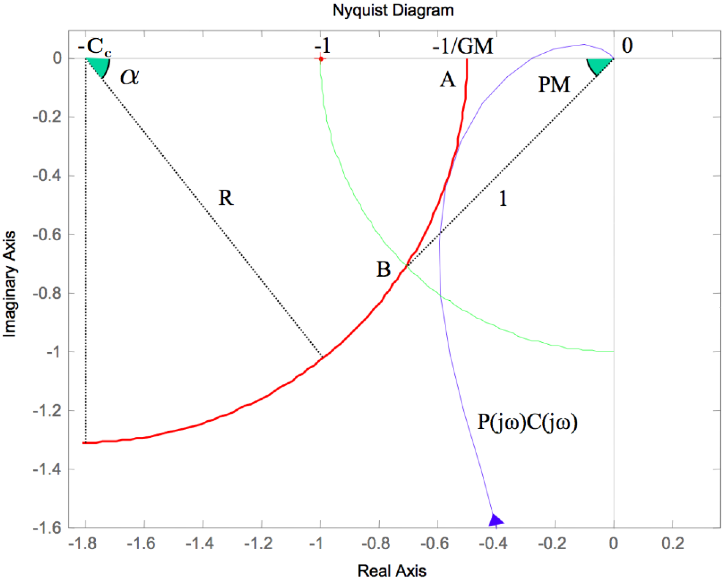
A simple auto-tuning method is used in this paper to design a PID controller using solely the frequency response and its corresponding frequency response slope of the robot at a specific frequency $\overline{\omega }$. This auto-tuning method is called the KC auto-tuner and produces robust PID controllers [25]. The basic idea of the KC auto-tuning method is based on defining a circular region, including the $-1$ point in the Nyquist plane. This circular region is defined as a “forbidden region”, which is a circle computed according to two design constraints: the gain margin (GM = 2) and the phase margin (PM = 45°); see Figure 11. The main design requirement is that the loop frequency response $L\left(s\right)=P\left(s\right)C\left(s\right)$ needs to avoid entering the forbidden region, and most importantly, the robust PID controller parameters are determined in such a way as to ensure that the slope-difference between the circle border and the loop frequency response is minimum:

$$\underset{\alpha }{min}∥{\left.\frac{dIm}{dRe}\right|}_{\alpha }-{\left.\frac{d{\Im }_L}{d{\Re }_L}\right|}_{\overline{\omega }}∥,0\le \alpha \le {\alpha }_{max}$$

(40)

where ${\left.\frac{d{\Im }_L}{d{\Re }_L}\right|}_{\omega =\overline{\omega }}$ is the slope of the loop frequency response in the Nyquist plane and ${\left.\frac{dIm}{dRe}\right|}_{\alpha }$ is the slope of the “forbidden region” border, as a function of the angle $\alpha$, as indicated in Figure 11.

To compute ${\left.\frac{d{\Im }_L}{d{\Re }_L}\right|}_{\omega =\overline{\omega }}$, the slope of the loop frequency response has to be evaluated firstly as:

$${\left.\frac{dL\left(j\omega \right)}{d\omega }\right|}_{\omega =\overline{\omega }}=P\left(j\overline{\omega }\right){\left.\frac{dC\left(j\omega \right)}{d\omega }\right|}_{\omega =\overline{\omega }}+C\left(j\overline{\omega }\right){\left.\frac{dP\left(j\omega \right)}{d\omega }\right|}_{\omega =\overline{\omega }}$$

(41)

The process frequency response $P\left(j\overline{\omega }\right)$ and the process frequency response slope ${\left.\frac{dP\left(j\omega \right)}{d\omega }\right|}_{\omega =\overline{\omega }}$ are determined as mentioned in Section 3.1 and Section 3.2. Furthermore, for a user-specified frequency $\overline{\omega }$, the frequency response of the PID controller can be determined according to:

$$C\left(j\overline{\omega }\right)=\frac{L\left(j\overline{\omega }\right)}{P\left(j\overline{\omega }\right)}$$

(42)

whereas ${\left.\frac{dC\left(j\omega \right)}{d\omega }\right|}_{\omega =\overline{\omega }}$ is easily calculated in a numerical way for a known controller $C\left(s\right)$ [25].

In this way, the slope of the loop frequency response in (41) can be easily broken into a real ${\Re }_L$ and an imaginary ${\Im }_L$ part as:

$${\left.\frac{dL\left(j\omega \right)}{d\omega }\right|}_{\omega =\overline{\omega }}={\left.\frac{d{\Re }_L}{d\omega }\right|}_{\omega =\overline{\omega }}+j{\left.\frac{d{\Im }_L}{d\omega }\right|}_{\omega =\overline{\omega }}$$

(43)

Then, the slope of the loop frequency response in the Nyquist plane can be computed as the ratio ${\left.\frac{d{\Im }_L}{d{\Re }_L}\right|}_{\omega =\overline{\omega }}$. Regarding Figure 11, it is obvious that any point of the forbidden region circle is defined by the radius R and the angle $\alpha$. Computing the real and imaginary parts of this point in the Nyquist plane, the following equations are obtained:

$$Re\left(\alpha \right)=-C_c+Rcos\left(\alpha \right)\mathrm{and}Im\left(\alpha \right)=-Rsin\left(\alpha \right)$$

(44)

The equation of the circle in that same point gives:

$${\left(Re\left(\alpha \right)+C_c\right)}^2+Im{\left(\alpha \right)}^2=R^2$$

(45)

with the derivative equal to:

$$2\left(Re\left(\alpha \right)+C_c\right)\left(dRe\right)+2Im\left(\alpha \right)\left(dIm\right)=0$$

(46)

Then slope of the “forbidden region” is determined using the result in (46):

$${\left.\frac{dIm}{dRe}\right|}_{\alpha }=-\frac{Re\left(\alpha \right)+C_c}{Im\left(\alpha \right)}=\frac{cos\left(\alpha \right)}{sin\left(\alpha \right)}$$

(47)

where the result in (44) has also been used. With the results in (43) and (47), the minimization problem in (40) is solved with a single for-loop where $\alpha$ varies from 0–α_max in 1° steps. Referring to Figure 11, it is obvious that ${\alpha }_{max}={90}^{\circ }$.

3.5. Tuning of the PID Controller

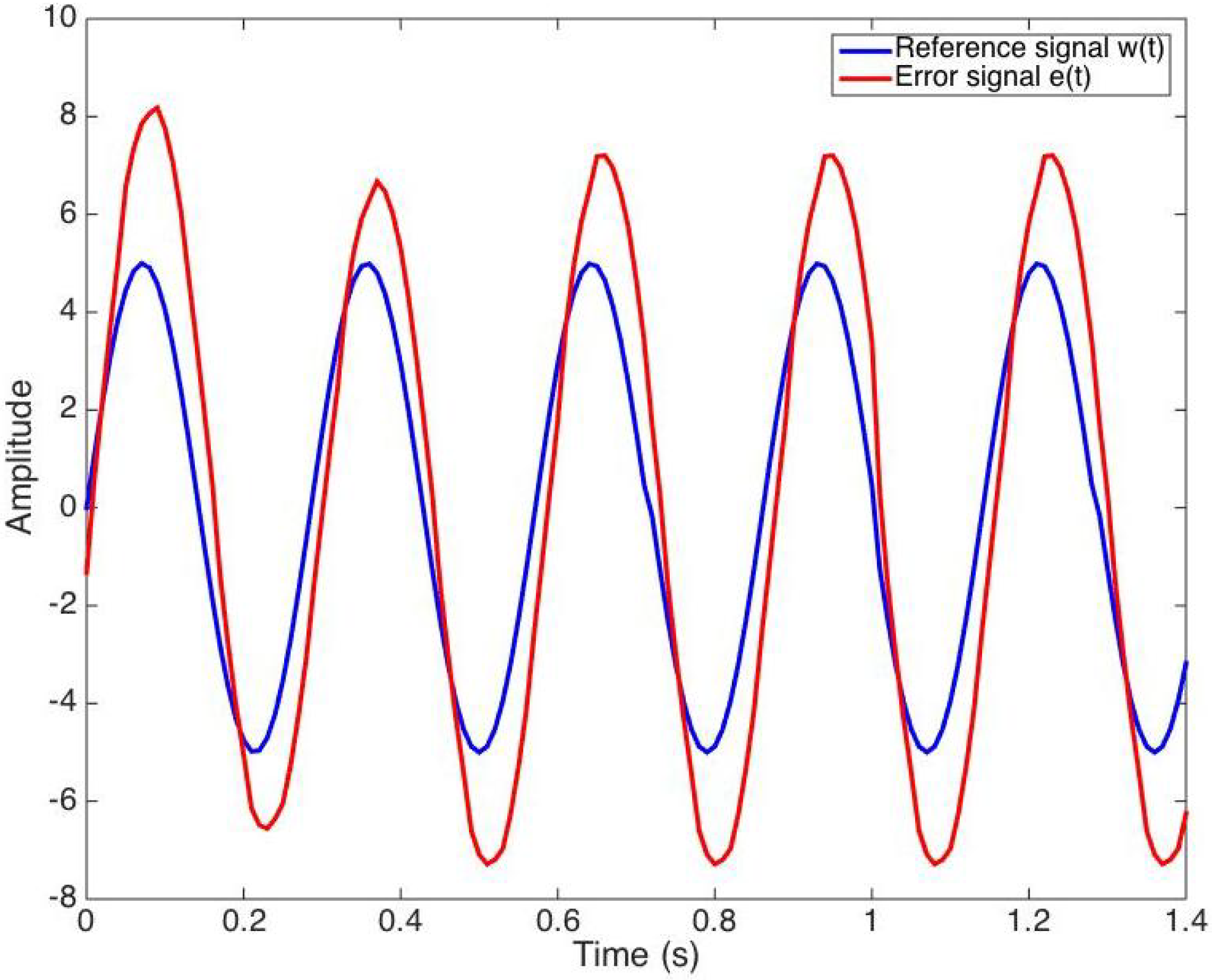
To tune the controller, the test frequency is selected as $\overline{\omega }=22$ rad/s, while the gain and phase margins are GM = 2 and PM = 45°. Firstly, in the KC auto-tuning method, the process frequency response and frequency response slope at the test frequency are required. For this purpose, a reference signal as indicated next is used and applied to Joints 2 and 3 of the robot, similarly to the procedure described in Section 3.3:

$$w\left(t\right)=A_{w}sim\left(\overline{\omega }t\right)$$

(48)

with $A_w=5$. The output signal is measured periodically, and the error signal is computed as:

$$e\left(t\right)=w\left(t\right)-y\left(t\right)$$

(49)

The reference and error signals are indicated in Figure 12.

The steady-state component of the error signal can be written simply as:

$$e_{SS}\left(t\right)=A_{e}sin(\overline{\omega }t+{\phi }_e)=7.4sin(\overline{\omega }t-0.33)$$

(50)

and since there is no stochastic disturbance, it can be determined “graphically”. Figure 13 shows the reference and error signals measured experimentally, along with the steady state component in (50). The transient component of the error signal is simply determined as the difference:

$$e_{tr}\left(t\right)=e\left(t\right)-e_{SS}\left(t\right)$$

(51)

and it is given in Figure 14.

Next, the discrete Fourier transform is used to evaluate the following integral, as in (34):

$${\int }_0^{\infty }{e}_{TR}\left(t\right)e^{-j\overline{\omega }t}dt=T_s\sum _{k=0}^{N-1}{e}_{TR}\left(k{T}_s\right)e^{-j\overline{\omega }k{T}_s}$$

(52)

a result that is finally used in an equation similar to (33) to compute the amplitude $A_{\overline{x}}$ and phase ${\phi }_{\overline{x}}$:

$$A_{\overline{x}}{e}^{j{\phi }_{\overline{x}}}=2j{\int }_0^{\infty }{e}_{TR}\left(t\right)e^{-j\overline{\omega }t}dt$$

(53)

Then, using the result in Figure 8 for the derivative of the error signal $\overline{e}\left(t\right)$ leads to a means of computing the amplitude $A_{\overline{e}}$ and phase ${\phi }_{\overline{e}}$ of the signal $\overline{e}\left(t\right)$ at the specific frequency $\overline{\omega }$ as:

$$A_{\overline{e}}{e}^{j{\phi }_{\overline{e}}}=A_{\overline{x}}{e}^{j{\phi }_{\overline{x}}}+\frac{A_{e}sin\left({\phi }_e\right)}{\overline{\omega }}=-0.109+0.0042j$$

(54)

with $A_e=7.4$ and ${\phi }_e=-0.33$ rad/s, as indicated in (50).

With the result in (54), the following is obtained by modifying (24):

$${\left.\frac{dS\left(j\omega \right)}{d\left(j\omega \right)}\right|}_{\omega =\overline{\omega }}=j\frac{A_{\overline{e}}}{A_w}{e}^{j{\phi }_{\overline{e}}}=-0.00084-0.0218j$$

(55)

The frequency response of $S\left(s\right)$ at the test frequency $\overline{\omega }$ is computed similarly to the equation in (10) as:

$$S\left(j\overline{\omega }\right)=\frac{A_e}{A_w}{e}^{j{\phi }_e}=1.4-0.48j$$

(56)

The process frequency response $P\left(j\overline{\omega }\right)$ can be easily determined using (36) and the result in (56), considering that the controller used is P-type with $C\left(j\overline{\omega }\right)=15$:

$$P\left(j\overline{\omega }\right)=\frac{1-S\left(j\overline{\omega }\right)}{1-C\left(j\overline{\omega }\right)S\left(j\overline{\omega }\right)}=-0.024+0.0145j$$

(57)

The process frequency response slope is computed according to (39):

$${\left.\frac{dP\left(j\omega \right)}{d\omega }\right|}_{\omega =\overline{\omega }}=-3.86\ast {10}^{-4}+5.4\ast {10}^{-4}j$$

(58)

The resulting PID controller, computed according to the KC auto-tuning procedure described in Section 3.4, is the following:

$$C\left(s\right)=9.42\left(1+\frac{1}{0.45s}+0.21s\right)$$

(59)

4. Experimental Results

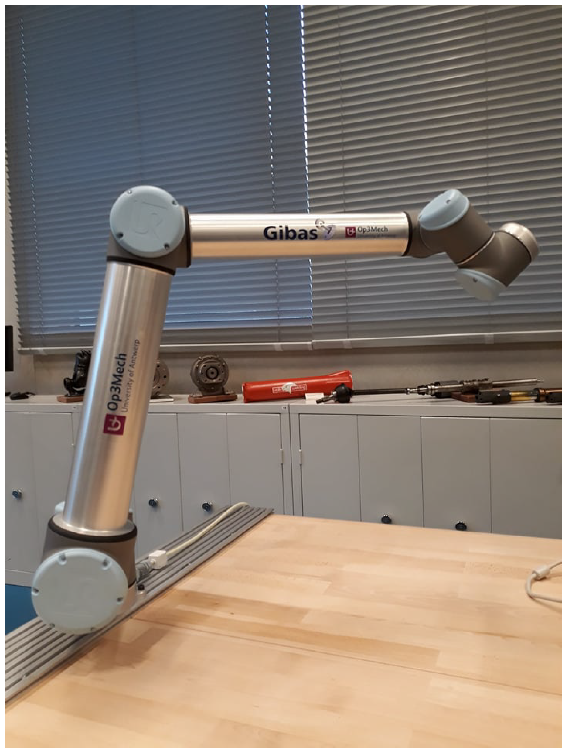
This section reports the experimental results that were achieved in order to validate the auto-tuning method of a PID controller, presented in the previous section. The performance of the obtained controllers has been evaluated in the real-time application using the setup depicted in Figure 15. In order to communicate with the UR10 robot, the Robotics System Toolbox of MATLAB® and the ROS platform were used.

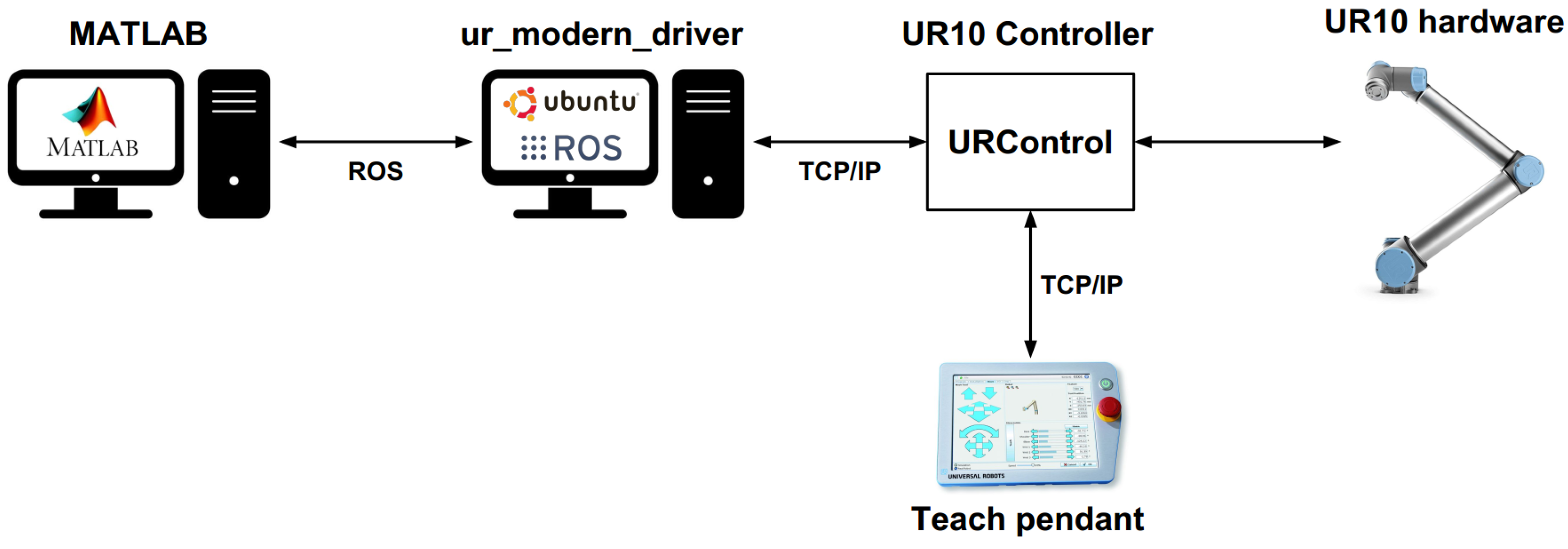
The UR10 controller uses Ethernet and the TCP/IP protocol to send and receive commands. The control and calculations of the robot are executed in MATLAB®. Although it is possible to send commands directly from MATLAB® to the controller, it was chosen to use the ROS platform for a more versatile solution. Therefore, the ROS-supported ur_moder_driver runs on a computer with a Linux operating system, which is directly connected to the robot controller through TCP/IP. The ur_modern_driver allows an easy communication with many different operating systems and publishes robot data with the use of ROS messages. As MATLAB® has a built-in ROS support, this ensures a very clear and effortless communication; for more details, please see [32]. An overview of the complete communication model is given in Figure 16. The running nodes and topics within the ROS platform related to this case study are illustrated in Figure 17.

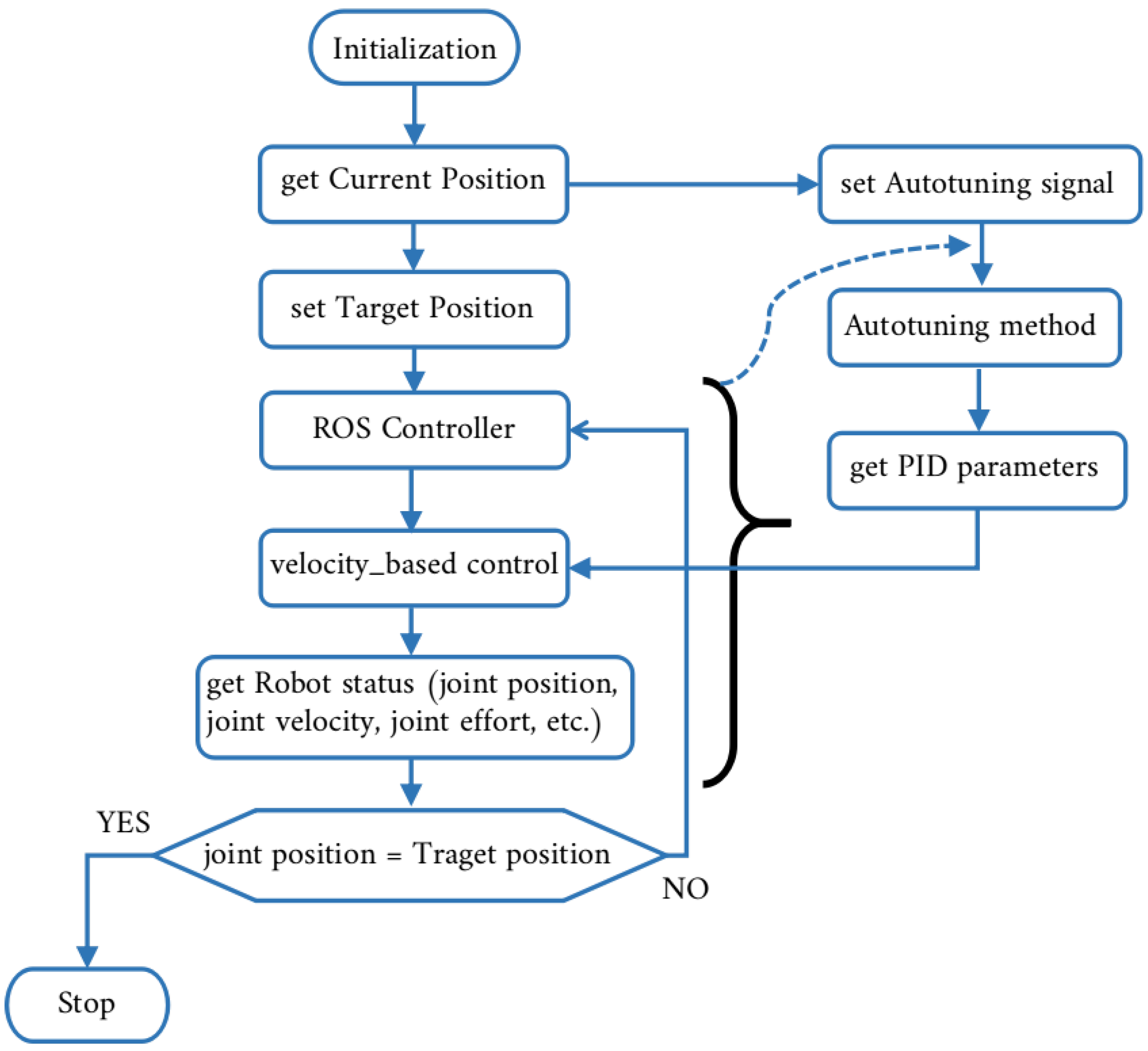
The procedure used to control the movements of the robot is presented in the flowchart in Figure 18. Notice that the auto-tuning method implies the use of $ROS-controller$ and velocity_based_controller, as well. Besides controlling the movements of the robot, it is very important to have access to the status of the robot’s joint states (joint position, joint velocity, joint effort, etc.). Thus, it can be mentioned that implementing a new controller on an industrial robot is strongly dependent on the opening level of the robot controller and the type of the driver used. In order to implement the auto-tuning method presented in this paper it is required to have read/write access to the joint states of the robot.

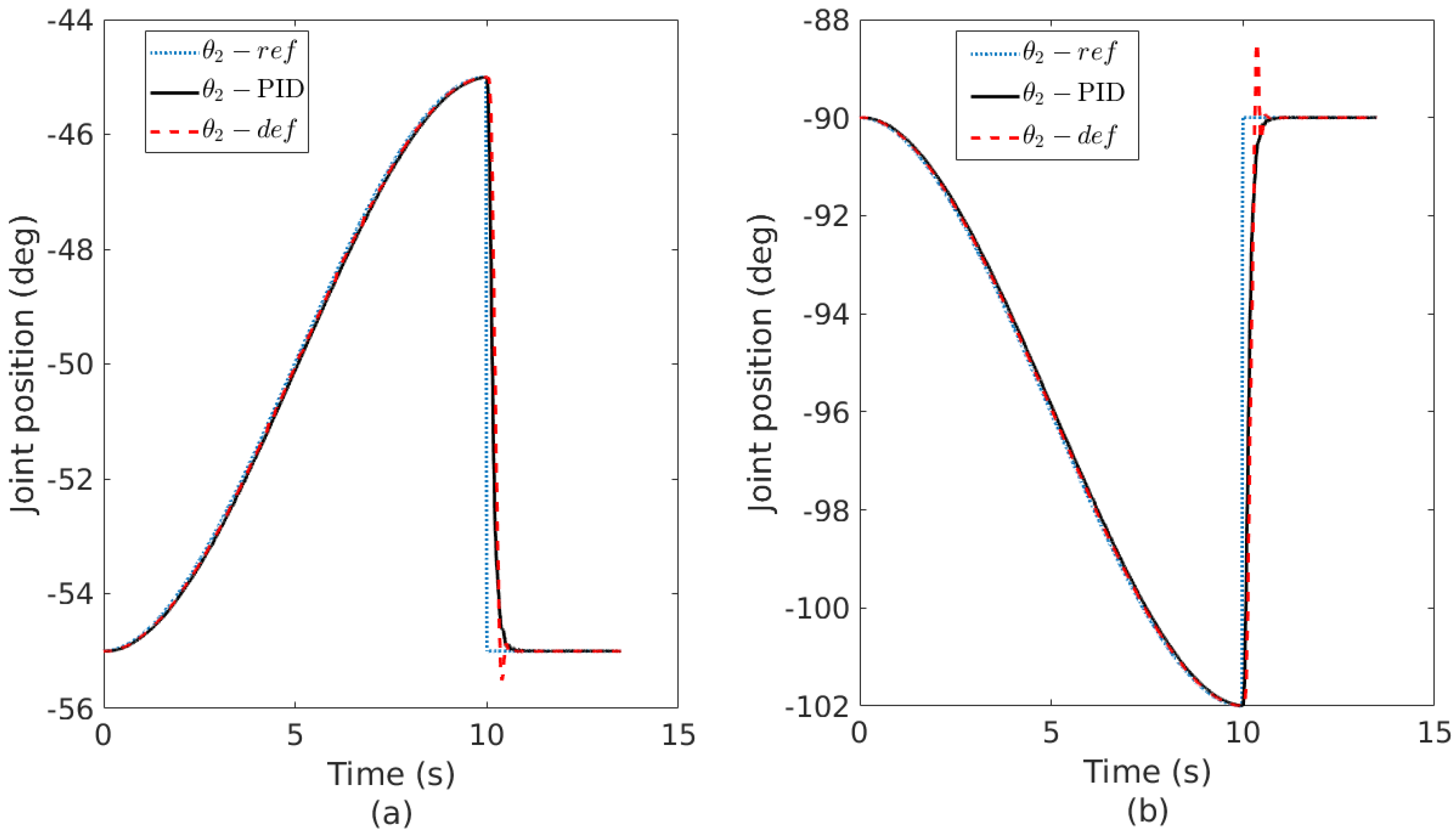
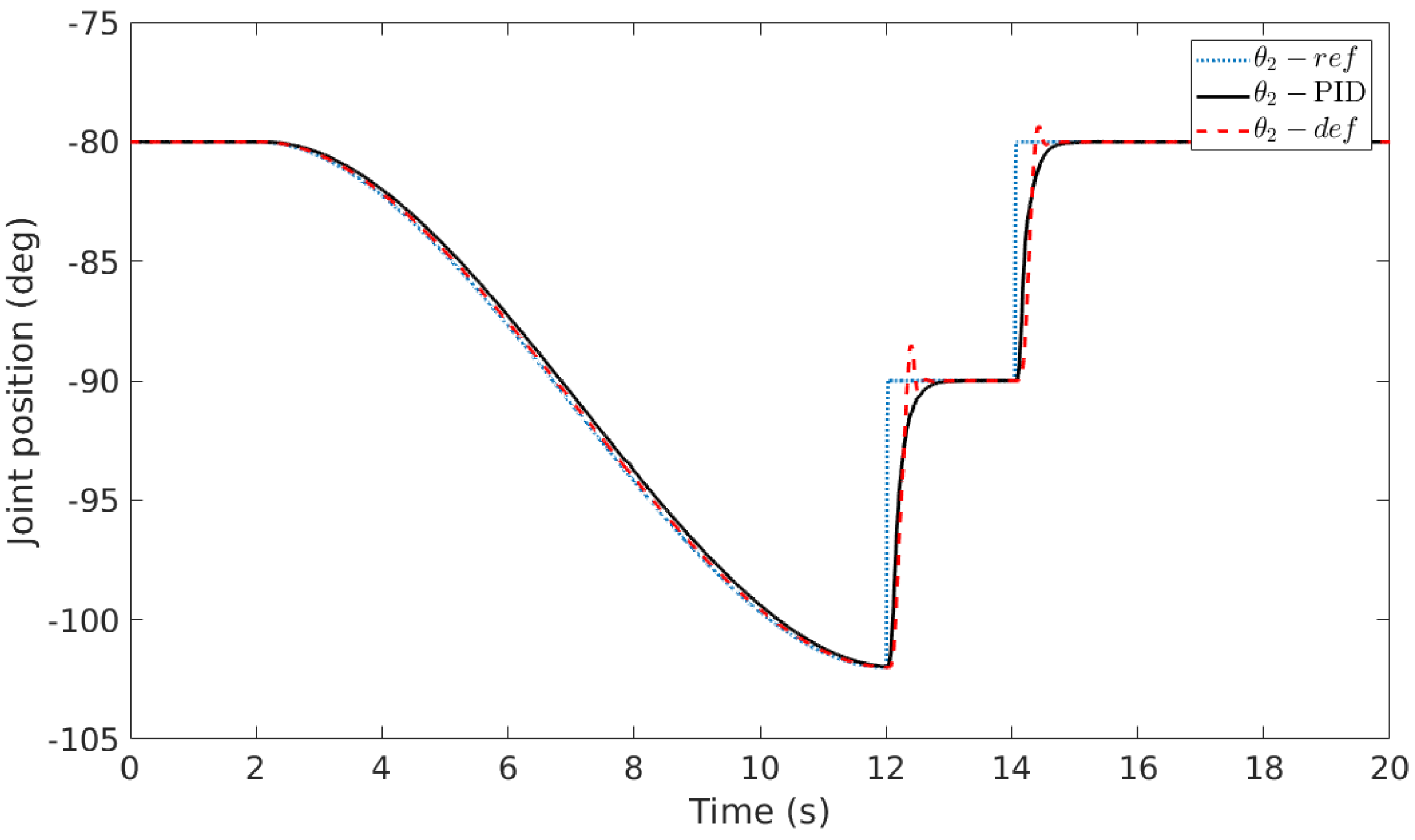
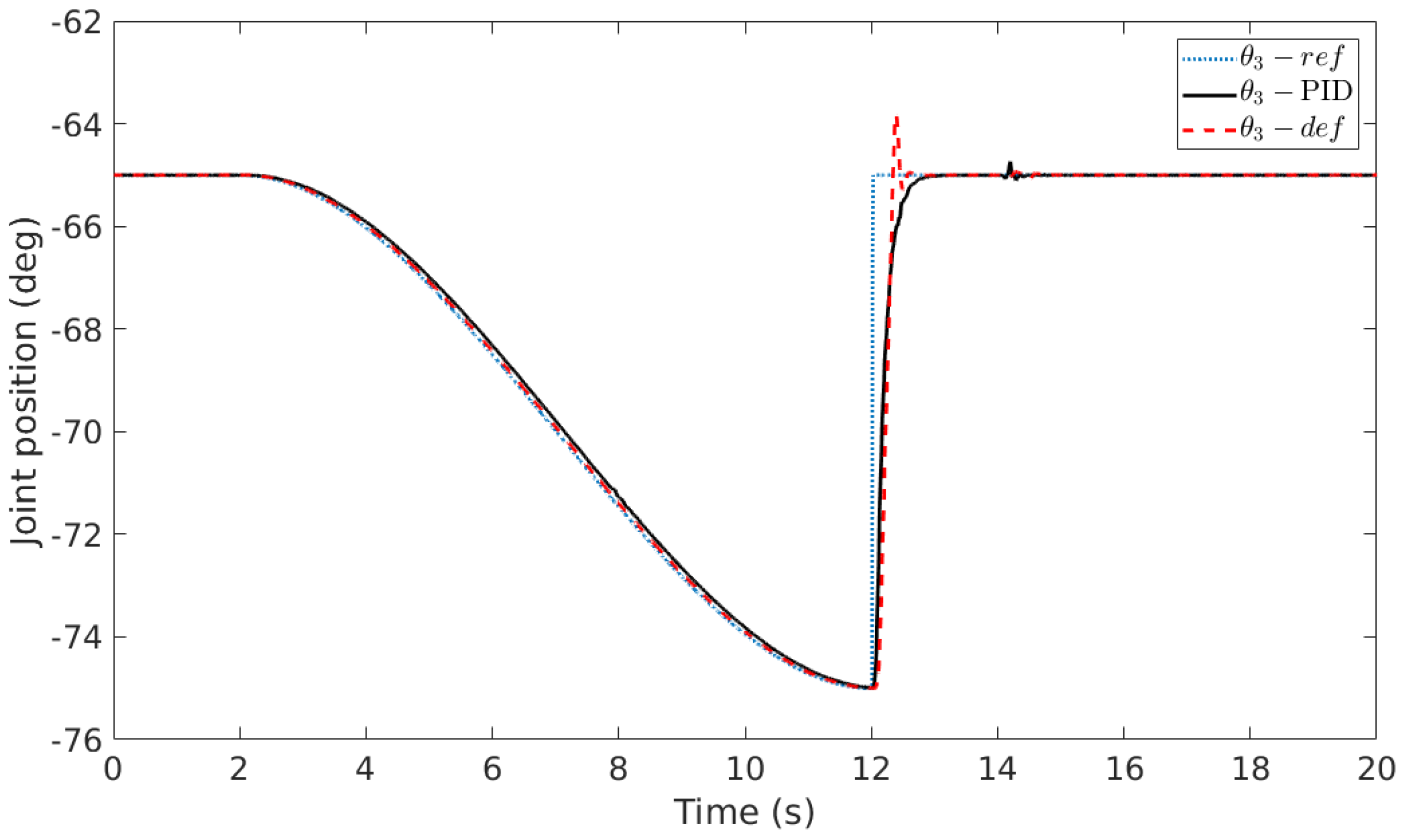
The speed control was developed and applied to Joint 2 and Joint 3 of the manipulator robot (these two joints have a larger variation compared with other joints). The controller was tested for multiple scenarios and different configurations of the manipulated robot. The first test was conducted using the following configuration $[-80,-45,-50,-80,260,-90]$, and the obtained results are presented in Figure 19a and Figure 20a. The output of the manipulator robot for the second configuration ($[35,-102,-75,90,-120,110]$) considered in this paper is presented in Figure 19b and Figure 20b. The third test case presented in this paper is illustrated in Figure 21 and Figure 22. As observed, the controller performs equally for different joint configurations, while keeping the interaction between joints at a minimum. It can be seen that the PID controller designed using the proposed auto-tuning procedure converges to the imposed reference for all considered cases and presents no overshoot in comparison with the available controller. Given the problem addressed in this paper, the results provided indicate that the auto-tuning method can be successfully applied in the field of robotic control.

5. Conclusions

In this paper, a PID based on a single sine test auto-tuning method was designed and implemented for a robot system. Due to the advantage of the auto-tuning approach, which ensures that the difference between the slope of the region border in the Nyquist plane and the loop frequency response slope are minimum, the obtained PID controller is robust to gain, phase and delay variations. This robustness is highly demanded for a manipulator robot taking into account its dynamics (variation with respect to the position and orientation of the robot). The outcome of this paper shows that the proposed technique is a suitable method for tuning PID controllers. The experimental results indicate an increased performance of the manipulator robot when the proposed auto-tuning technique is used. Even more, this method could bring a benefit for both real-life and industrial applications given that it is time saving and is easy to use by non-experts in control engineering.

References

- Spong, M.; Hutchinson, S.; Vidyasagar, M. Robot Modeling and Control; Wiley: Hoboken, NJ, USA, 2006. [Google Scholar]
- Bishop, R. The Mechatronics Handbook; CRC Press: Boca Raton, FL, USA, 2002. [Google Scholar]
- Steinbuch, M.; Merry, R.; Boerlage, M.; Ronde, M.; van de Molengraft, M. Advanced Motion Control Design. In The Control Handbook: Control System Application; Levin, W.S., Ed.; CRC Press: Boca Raton, FL, USA, 2010. [Google Scholar]
- Steinbuch, M.; Schootstra, G.; Bosgra, O. Robust control of a compact disc mechanism. In Control System Applications; Levine, W.S., Ed.; CRC Press: Boca Raton, FL, USA, 2000. [Google Scholar]
- Astrom, K.; Hagglund, T. Advanced PID Control; ISA-The Instrumentation, Systems, and Automation Society: Durham, NC, USA, 2006. [Google Scholar]
- Ionescu, C.; Copot, C.; Verellen, D. Motion compensation for robotic lung tumour radiotherapy in remote locations: A personalised medicine approach. Acta Astronaut. 2017, 132, 59–66. [Google Scholar] [CrossRef]
- Sayeh, S.; Wang, J.; Main, W.; Kilby, W.; Maurer, C.R., Jr. Respiratory motion tracking for robotic radiosurgery. In Treating Tumours that Move with Respiration; Urschel, H.C., Jr., Ed.; Springer: Berlin/Heidelberg, Germany, 2007; pp. 15–29. [Google Scholar]
- Seppenwoolde, Y.; Berbeco, R.; Nishioka, S.; Shirato, H.; Heijmen, B. Accuracy of tumour motion compensation algorithm from a robotic respiratory tracking system a simulation study. Med. Phys. 2007, 34, 2774–2784. [Google Scholar] [CrossRef] [PubMed]
- Tang, X.; Liu, Y.; Lv, C.; Sun, D. Hand Motion Classification Using a Multi-Channel Surface Electromyography Sensor. Sensors 2012, 12, 1130–1147. [Google Scholar] [CrossRef] [PubMed] [Green Version]
- Raya, R.; Rocon, E.; Gallego, J.; Ceres, R.; Pons, J. A Robust Kalman Algorithm to Facilitate Human-Computer Interaction for People with Cerebral Palsy, Using a New Interface Based on Inertial Sensors. Sensors 2012, 12, 3049–3067. [Google Scholar] [CrossRef] [PubMed] [Green Version]
- Yan, R.; Tee, K.; Li, H. Nonlinear control of a robot manipulator with time-varying uncertainties. In Proceedings of the Second International Conference on Social Robotics (ICSR), Singapore, 23–24 November 2010; pp. 202–211. [Google Scholar]
- Xu, J.; Viswanathan, B.; Qu, Z. Robust learning control for robotic manipulators with an extension to a class of non-linear systems. Int. J. Control 2000, 76, 858–870. [Google Scholar] [CrossRef]
- Xian, B.; Dawson, D.; Queiroz, M.; Chen, J. A continuous asymptotic tracking control strategy for uncertain nonlinear systems. IEEE Trans. Autom. Control 2004, 49, 1206–1211. [Google Scholar] [CrossRef]
- Busoniu, L.; Schutter, B.; Babuska, R. Decentralized reinforcement learning control of a robotic manipulator. In Proceedings of the 9th International Conference on Control, Automation, Robotics and Vision, Singapore, 5–8 December 2006; pp. 1347–1352. [Google Scholar]
- Bouakrif, F.; Boukhetala, D.; Boudjema, F. Velocity observer-based iterative learning control for robot manipulators. Int. J. Syst. Sci. 2013, 44, 214–222. [Google Scholar] [CrossRef]
- Delchev, K.; Boiadjiev, G.; Kawasaki, H.; Mouri, T. Iterative learning control with sampled-data feedback for robot manipulators. Int. J. Arch. Control Sci. 2014, 24, 299–319. [Google Scholar] [CrossRef] [Green Version]
- Astrom, K.; Hagglund, T. Automatic tuning of simple regulators with specifications on phase and amplitude margins. Automatica 1984, 20, 645–651. [Google Scholar] [CrossRef] [Green Version]
- Tan, K.; Lee, T.; Wang, Q. Enhanced automatic tuning procedure for process control of PI/PID controllers. AlChE J. 1996, 42, 2555–2562. [Google Scholar] [CrossRef]
- Chen, Y.; Moore, K. Relay feedback tuning of robust PID controllers with iso-damping property. Trans. Syst. Man. Cybern. 2005, 35, 23–31. [Google Scholar] [CrossRef]
- Hagglund, T.; Astrom, K. Revisiting the Ziegler—Nichols tuning rules for PI control. Asian J. Control 2002, 4, 364–380. [Google Scholar] [CrossRef]
- Akkermans, S.; Stan, S. Digital servo IC for optical disc drives. Control Eng. Pract. 2002, 9, 1245–1253. [Google Scholar] [CrossRef]
- Panagopoulos, H.; Astrom, K.; Hagglund, T. Design of PID controllers based on constrained optimisation. IEEE Proc. Control Theory Appl. 2002, 149, 32–40. [Google Scholar] [CrossRef]
- Astrom, K.; Hagglund, T. Revisiting the Ziegler—Nichols step response method for PID control. J. Process. Control 2004, 14, 635–650. [Google Scholar] [CrossRef]
- Skogestad, S. Simple analytic rules for model reduction and PID controller tuning. J. Process. Control 2003, 13, 291–309. [Google Scholar] [CrossRef] [Green Version]
- De Keyser, R.; Ionescu, C.; Muresan, C. Comparative Evaluation of a Novel Principle for PID Autotuning. In Proceedings of the Asian Control Conference, Gold Coast, Australia, 17–20 December 2017; pp. 1164–1169. [Google Scholar]
- De Keyser, R.; Muresan, C.; Ionescu, C. A single sine test can robustly estimate a system’s frequency response slope. Int. J. Syst. Sci. 2018. submitted. [Google Scholar]
- Corke, P. Robotics, Vision & Control; Springer: Berlin/Heidelberg, Germany, 2011. [Google Scholar]
- Siciliano, B.; Sciavicco, L.; Villani, L.; Oriolo, G. Robotics, Modelling, Planning and Control; Springer: Berlin/Heidelberg, Germany, 2009. [Google Scholar]
- Naumovic, M.; De Keyser, R.; Robayo, F.; Ionescu, C. Developing Frequency Response Analyzer in MATLAB® Simulink Environment. In Proceedings of the 17th Telecommunications Forum TELFOR, Belgrade, Serbia, 24–26 November 2009; pp. 701–704. [Google Scholar]
- De Keyser, R.; Ionescu, C.; Festila, C. A One-Step Procedure for Frequency Response Estimation based on a Switch-Mode Transfer Function Analyzer. In Proceedings of the 50th IEEE Conference on Decision and Control and European Control Conference (CDC-ECC), Orlando, FL, USA, 12–15 December 2011; pp. 1189–1194. [Google Scholar]
- De Keyser, R.; Muresan, C.; Ionescu, C. A Novel Auto-tuning Method for Fractional Order PI/PD Controllers. ISA Trans. 2016, 62, 268–275. [Google Scholar] [CrossRef] [PubMed]
- Andersen, T.T. Optimizing the Universal Robots ROS Driver; Technical Report; Department of Electrical Engineering, Technical University of Denmark: Lyngby, Denmark, 2015. [Google Scholar]
Figure 1.
Schematic overview of the UR10 robot: CAD model.
Figure 2.
Gravity load variation of a UR10 robot; (a) joint 2 gravity load, and (b) joint 3 gravity load, .
Figure 3.
Inertia matrix variation of a UR10 robot.
Figure 4.
Schematic overview of a classical robot joint drivetrain.
Figure 5.
The structure of the nested control architecture.
Figure 6.
The basic scheme for determining the frequency response slope.
Figure 7.
The robust scheme for determining the frequency response slope: (a) intermediary solution; (b) final solution.
Figure 8.
Simplified robust scheme for determining the frequency response slope.
Figure 9.
Closed loop scheme for determining the frequency response of a process and the frequency response slope.
Figure 10.
Simplified closed loop scheme for determining the frequency response of and the corresponding frequency response slope.
Figure 11.
The loop frequency response (blue line) and the ‘forbidden region’ (red circle). GM, gain margin; PM, phase margin.
Figure 12.
Reference and error signals measured experimentally.
Figure 13.
Reference and steady state error signals used to determine the robot frequency response and its corresponding slope.
Figure 14.
Transient component of the error signals used to determine the robot frequency response and its corresponding slope.
Figure 15.
The UR10 robot available in our laboratory.
Figure 16.
Communication model of the data transmission between the UR10 robot and the MATLAB® software.
Figure 17.
Visualization of the ROS computation graph.
Figure 18.
The flowchart for controlling the movements of the robot.
Figure 19.
Step response of the UR10 robot for Joint 2(PID, the designed controller; def, the default controller available on the robot); (a) first robot configuration and (b) second robot configuration.
Figure 20.
Step response of the UR10 robot for Joint 3; (a) first robot configuration and (b) second robot configuration.
Figure 21.
Response of the UR10 robot for Joint 2.
Figure 22.
Response of the UR10 robot for Joint 3.