Robust Interval Type-2 Fuzzy Sliding Mode Control Design for Robot Manipulators

Abstract

This paper develops a new robust tracking control design for n-link robot manipulators with dynamic uncertainties, and unknown disturbances. The procedure is conducted by designing two adaptive interval type-2 fuzzy logic systems (AIT2-FLSs) to better approximate the parametric uncertainties on the system nominal. Then, in order to achieve the best tracking control performance and to enhance the system robustness against approximation errors and unknown disturbances, a new control algorithm, which uses a new synthesized AIT2 fuzzy sliding mode control (AIT2-FSMC) law, has been proposed. To deal with the chattering phenomenon without deteriorating the system robustness, the AIT2-FSMC has been designed so as to generate three adaptive control laws that provide the optimal gains value of the global control law. The adaptation laws have been designed in the sense of the Lyapunov stability theorem. Mathematical proof shows that the closed loop control system is globally asymptotically stable. Finally, a 2-link robot manipulator is used as case study to illustrate the effectiveness of the proposed control approach.

1. Introduction

The tracking control problem of robot manipulators is a very complicated issue due to undesirable characteristics, such as high nonlinearities, strong dynamic coupling, parameter perturbations, un-modeled dynamics, and unknown disturbances. Therefore, to achieve the good tracking control performance for such complex process, several researchers have developed robust control approaches, most of which use the fuzzy logic control (FLC), sliding mode control (SMC), feedback linearization technique, Neural Network (NN), adaptive control, and $H_{\infty }$ technique [1,2,3,4,5,6,7,8,9,10,11].

Over the past years, intelligent algorithms using fuzzy logic systems (FLSs) are increasingly used and successfully applied in control problem of robot manipulators in the presence of dynamic uncertainties and unknown disturbances [12,13,14]. However, conventional type-1 fuzzy logic system (T1-FLS) cannot directly handle rule and measurement uncertainties because it uses T1-fuzzy sets (T1-FSs) that are certain. Therefore, these last years, an advanced form of FLS, called type-2 FLS (T2-FLS), has attracted considerable attention and becomes more and more imposed in designing robust controllers for uncertain complex processes, including robot systems [15,16,17,18]. One reason is that a T2-FS is characterized by a membership function (MF) that includes a footprint of uncertainty (FOU), which makes it possible to handle linguistic uncertainties more effectively than T1-FS [19,20,21].

On the other hand, SMC is known as an efficient tool well suitable for controlling complex uncertain processes due to its higher robustness against dynamic uncertainties and unknown disturbances [22,23,24]. However, the SMC has a major drawback, which consists in using a discontinuous control law with large control gains that generate the chattering [25]. This phenomenon can cause severe damage to system actuators. In order to overcome or reduce the chattering, boundary layer method (BL), and higher order SMC approach (HO-SMC) are commonly employed by many researchers [26,27,28,29,30,31]. However, these approaches have a drawback that limits their performance, which consists in the fact that they still require the knowledge of the upper bounds of the uncertainties to ensure the desired control performance. The overestimation of the control gains to cover a wide range of uncertainties can cause the chattering and a dynamic response with overshoot, and the small gains can deteriorate the control accuracy performance and affect the system robustness. Moreover, BL method constrains the system trajectories not to the desired dynamics, but to their vicinities, thus both the control accuracy and robustness are affected. The HO-SMC approach requires in general higher order derivative of the sliding variable. The second order super-twisting SMC (SOST-SMC) is among the most effective HO-SMC algorithms that is widely used in the literature for controlling complex uncertain processes [4,32,33,34,35], it is developed by Levant [36] to avoid the chattering and to ensure the finite time convergence of the system state trajectories. However, the choice of its optimal control gains values remains a challenging matter for this kind of controllers.

In order to increase accurate tracking control performance and to guarantee the robustness of robot manipulators against dynamic uncertainties and unknown disturbances, several approaches have been developed. Among them, those that combine the benefits of FLS and robust control techniques, such as SMC, $H_{\infty }$ Technique, NN, and adaptive control have recently been the focus of many researchers [37,38,39]. In [40], a FLS and a fuzzy sliding mode controller are employed to achieve the best tracking performance for the robot manipulators in presence of uncertainties. Most recently, in [41], the authors used an adaptive fuzzy sliding mode controller in order to improve the precision trajectory tracking of a designed winding hybrid-driven cable parallel manipulator subject to un-modeled dynamics and random disturbances. In [42], in order to regulate the vertical displacement of a bioinspired robotic dolphin, a sliding mode fuzzy control method is successfully applied. In [43], a hierarchically improved fuzzy dynamical sliding-model control is proposed for the autonomous ground vehicle to ensure the best path tracking performance in the presence of different payloads.

When compared to the existing works in the literature, the main contributions of the present study are listed, as follows:

(1)

a new robust algorithm is proposed for n-link robot manipulator systems to deal with the tracking control problems, with the following considerations are taken into account:

• The dynamics of the robot manipulator systems are only partially known and present parametric variations.
• The studied systems are subject to unknown disturbances.
• No prior knowledge of the upper bound of the parametric uncertainties, unknown dynamics, un-modeled dynamics, and unknown disturbances that affect the studied system dynamics is required.

(2)

Based on T2-FLS, two adaptive interval T2-FLSs (AIT2-FLSs) are designed in order to efficiently estimate the parametric uncertainties of the system dynamics. FSs are chosen to be interval T2 (IT2), firstly, because they do not require a lot of computation, and, secondly, for their efficiency to capture severe uncertainties.

(3)

In order to handle errors approximation of parametric uncertainties and effectively reject the effects of unknown dynamics, un-modeled dynamics, and unknown disturbances on the control system without generating the undesired chattering, a new enhanced robust AIT2-FSMC law is designed so as to generate three adaptive control laws in order to provide the optimal estimation of the control law gains that effectively reject all of the undesired effects that perturb the control system while yielding a smooth global control law. Thus, the best tracking control performance is guaranteed. The adaptation laws of the synthesized controller parameters have been designed in the sense of the Lyapunov stability approach. Finally, a 2-link robot manipulator is used as a study case to validate the effectiveness of the proposed control approach.

The rest of the paper is organized as follows. In Section 2, the problem formulation is presented. In Section 3, we propose the controller design method for n-link uncertain robot manipulator systems. Section 4 presents the simulation results for a robot manipulator system to illustrate the superiority of the proposed control approach in achieving the desired performance.

2. Problem Formulation

The main objective of this study is to design an enhanced tracking control for n-link robot manipulators in the presence of un-modelled dynamics, unknown payload dynamics, unknown friction force, parametric variations, and other unknown perturbations. The Euler-Lagrange dynamic equation for n-link robot manipulator systems can be written as:

$$J(q)\ddot{q}+C(q,\dot{q})\dot{q}+F(\dot{q})+G(q)=u+d$$

(1)

where $q,\dot{q},\ddot{q}\in {ℝ}^n$ are the vectors of joint angular position, velocity, and acceleration, respectively; $J(q)=\left(J_0(q)+\Delta J(q)\right)\in {ℝ}^{n\times n}$ is the bounded symmetric positive definite inertia matrix; $C(q,\dot{q})=\left(C_0(q,\dot{q})+\Delta C(q,\dot{q})\right)\in {ℝ}^n$ is the vector of centripetal Coriolis matrix; $G(q)=\left(G_0(q)+\Delta G(q)\right)\in {ℝ}^n$ denotes the gravity vector, with $J_0(q)$, $C_0(q,\dot{q})$, and $G_0(q)$ denote the nominal matrices, and $\Delta J(q)$, $\Delta C(q,\dot{q})$ and $\Delta G(q)$ represent the parametric variations on the nominal system; $F(\dot{q})\in {ℝ}^n$ is the unknown friction vector; $u\in {ℝ}^n$ represents the vector of input torques; $d\in {ℝ}^n$ is the disturbance vector including un-modelled dynamics, unknown payload dynamics, and other unknown perturbations.

The Equation (1) can be reformulated as:

$$\begin{array}{l}\ddot{q}=A(Q)+B(q)u+D\\ =A_0(Q)+B_0(q)u+\left(\Delta A(Q)+\Delta B(q)u\right)+D\end{array}$$

(2)

where $A(q,\dot{q})=A_0(q,\dot{q})+\Delta A(q,\dot{q})=-J^{-1}(q)\left(C(q,\dot{q})\dot{q}+G(q)\right)$, $B(q)=B_0(q)+\Delta B(q)=J^{-1}(q)$, and $D=J^{-1}(q)\left(d-F(\dot{q})\right)$, with $\Delta A(q,\dot{q})$ and $\Delta B(q)$ representing the parametric uncertainties on the system nominal, $Q\begin{array}{c}=\end{array}[\begin{array}{cc}{q}^T& {\dot{q}}^T\end{array}{]}^T\in {ℝ}^{2n}$ denotes the state vector of the system (1) assumed to be available to measurement, and $q=[\begin{array}{cccc}{q}_1& q_2& \dots & q_n\end{array}{]}^T$ is the first element of the state vector.

For convenience, it is assumed that: $\dot{J}(Q)-2C(Q)$ is skew symmetric, $J^{-1}(Q)$ exists, and $D$ is bounded.

3. Proposed Control Approach

3.1. Introduction to Type-2 Fuzzy Logic Systems

A T2-FLS is characterized by MFs that are themselves fuzzy. Output sets of inference engine are T2-FSs. Therefore, a reducer is required to convert them into T1-FS. The obtained type reducer set is then defuzzified to obtain a crisp output.

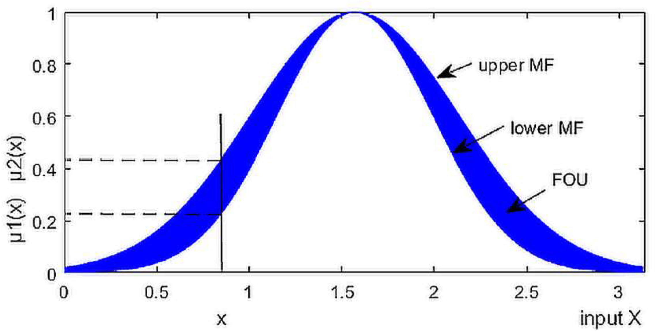
An example of a T2 fuzzy MF is the Gaussian MF represented in Figure 1, with the associated FOU being shown as a bounded blue area.

Upper MF and Lower MF are two T1 MFs. $\mu 1$ is the intersection of the crisp input $x$ with the lower MF, and $\mu 2$ is the intersection of $x$ with the upper MF.

3.1.1. Interval Type-2 Fuzzy System

For an IT2-FLS with a rule base of $M$ rules, each having $m$ antecedents, the jth rule can be expressed as [44]:

$$R^j:\mathrm{if}{x}_1\mathrm{is}{\tilde{F}}_1{}^j\mathrm{and}{x}_2\mathrm{is}{\tilde{F}}_2{}^j\dots \mathrm{and}{x}_m\mathrm{is}{\tilde{F}}_m{}^j\mathrm{then}y\mathrm{is}{\tilde{\theta }}_{}^j$$

(3)

where ${\tilde{F}}_i^j$ and ${\tilde{\theta }}_{}^j$ are IT2-FSs that are characterized by the fuzzy MFs ${\mu }_{{\tilde{F}}_i^j}(x_i)$ and ${\mu }_{{\tilde{\theta }}_{}^j}(y)$, respectively, ($j=1,2,\dots ,M$, $i=1,2,\dots ,m$); $X={\left[\begin{array}{cccc}{x}_1& x_2& \dots & x_m\end{array}\right]}^{}{}^T\in {ℝ}^m$ and $y\in ℝ$ are the input vector and the output of the IT2-FLS, respectively.

For the IT2-FLS described in (3), the meet operation is implemented by the product t-norm. Thus, the firing interval of the j-th fuzzy rule is the following IT1-FS:

$$Z^j(X)=\left[z_l^j(X),z_r^j(X)\right]$$

(4)

where $z_l^j(X)=\underset{i=1}{\overset{m}{\pi }}{\mu }_{{\tilde{F}}_i^j}^{low}(x_i)$ and $z_r^j(X)=\underset{i=1}{\overset{m}{\pi }}{\mu }_{{\tilde{F}}_i^j}^{upp}(x_i)$, with ${\mu }_{{\tilde{F}}_i^j}^{low}(x_i)$ and ${\mu }_{{\tilde{F}}_i^j}^{upp}(x_i)$ are the lower and upper MFs of ${\mu }_{{\tilde{F}}_i^j}(x_i)$, respectively.

3.1.2. Type Reduction for Interval Type-2 Fuzzy Sets

The output of the inference engine must be reduced to a T1-FS before defuzzification. The type reduction using the center of sets (COS) method is adopted in this study for the IT2-FSs and it is given by [45]:

$$Y_{\cos }\left({\theta }^1,{\theta }^2,\dots ,{\theta }^M,Z^1,Z^2,\dots ,Z^M\right)={\displaystyle \underset{y^1}{\int }{\displaystyle \underset{y^2}{\int }\dots {\displaystyle \underset{y^M}{\int }{\displaystyle \underset{z^1}{\int }{\displaystyle \underset{z^2}{\int }\dots {\displaystyle \underset{z^M}{\int }\frac{{\displaystyle \sum _{j=1}^M{z}^j}}{{\displaystyle \sum _{j=1}^M{y}^j{z}^j}}}}}}}}$$

(5)

where $Y_{\cos }$ is an IT1-FS defined by two end points $y_l(X)$ and $y_r(X)$; $y^j\in {\theta }^j=\left[{\theta }_l^j,{\theta }_r^j\right]$ with ${\theta }^j$is the centroid of the associated IT2 fuzzy consequent set ${\tilde{\theta }}_{}^j$; and, $z^j\in Z^j(X)=\left[z_l^j(X),z_r^j(X)\right]$.

The defuzzified crisp out by using the center of gravity is then obtained, as follows:

$$y=\frac{y_l+y_r}{2}$$

(6)

where $y_l$ and $y_r$ can be expressed as:

$$\{\begin{array}{l}{y}_l=\underset{Z^j}{\min }\frac{{\displaystyle \sum _{j=1}^M{\theta }_l^j}{z}^j}{{\displaystyle \sum _{j=1}^M{z}^j}}={\theta }_l^T{\xi }_l\\ y_r=\underset{Z^j}{Max}\frac{{\displaystyle \sum _{j=1}^M{\theta }_r^j}{z}^j}{{\displaystyle \sum _{j=1}^M{z}^j}}={\theta }_r^T{\xi }_r\end{array}$$

(7)

where ${\xi }_l={\left[\begin{array}{cccc}{\xi }_l^1& {\xi }_l^2& \dots & {\xi }_l^M\end{array}\right]}^{}{}^T$ and ${\xi }_r={\left[\begin{array}{cccc}{\xi }_r^1& {\xi }_r^2& \dots & {\xi }_r^M\end{array}\right]}^{}{}^T$ are two vectors of fuzzy basis functions, such that: ${\xi }_l^j=\frac{{\underset{\_}{z}}^j}{{\displaystyle \sum _{j=1}^M{\underset{\_}{z}}^j}}$ and ${\xi }_r^j=\frac{{\overline{z}}^j}{{\displaystyle \sum _{j=1}^M{\overline{z}}^j}}$, with (${\underset{\_}{z}}^j$, ${\overline{z}}^j$)$\in Z^j(X)$; ${\theta }_l={\left[\begin{array}{cccc}{\theta }_l^1& {\theta }_l^2& \dots & {\theta }_l^M\end{array}\right]}_{}^{}{}^T$ and ${\theta }_r={\left[\begin{array}{cccc}{\theta }_r^1& {\theta }_r^2& \dots & {\theta }_r^M\end{array}\right]}_{}^{}{}^T$ are the adjustable parameter vectors.

In this study, ${\underset{\_}{z}}^j$ and ${\overline{z}}^j$ are determined while using the iterative algorithm that was developed by Mendel and Karnik [46]. Therefore, $y_l$ and $y_r$ can be easily computed.

3.2. Control Law Design

In order to ensure that the state $q$ of the system (1) effectively tracks a desired reference $q_r$ in the presence of dynamic uncertainties and unknown disturbances without generating the chattering, a new robust AIT2-FSMC law is proposed.

3.2.1. Sliding Mode Control Law

The main objective of SMC is to force the system dynamics to reach and then remain on the sliding surface $s(Q,t)=\underset{\_}{0}$, with $\underset{\_}{0}\in {ℝ}^n$ denotes the null vector.

Define the tracking error $e=q_r-q$. Then, in order to ensure that the tracking error converges asymptotically to zero when the sliding surface $s(Q,t)=\underset{\_}{0}$ is established, we adopted in this study the following sliding surface defined by Slotine for a jth order system as [47]:

$$\begin{array}{cc}\hfill s(Q,t)& ={\left(\frac{\partial }{\partial t}+\lambda \right)}^{(p-1)}e\hfill \\ & ={\displaystyle \sum _{j=0}^{p-1}\frac{(p-1)!}{j!(p-j-1)!}}{\left(\frac{\partial }{\partial t}\right)}^{(p-j-1)}{\lambda }^{j}e\hfill \\ & =[s_1{s}_2\dots s_n{]}^T\in {ℝ}^n\hfill \end{array}$$

(8)

where $\lambda =diag{({\lambda }_i)}_{1\le i\le n}\in {ℝ}^{(n\times n)}$ is a diagonal matrix, with ${\lambda }_i$ is the positive slope of the sliding surface $s_i$; $p$ denotes the system order. In this study, for the system (1), we have $p=2$. Therefore:

$$s(Q,t)=\dot{e}+\lambda e$$

(9)

The time derivative of the above equation can be given, for the system (2), as:

$$\dot{s}(Q,t)={\ddot{q}}_r^{}-\left(A_0(Q)+B_0(q)u\right)-\left(\Delta A(Q)+\Delta B(q)u\right)-D+\lambda \dot{e}$$

(10)

In this paper, the IT2-FLS (6) is used to approximate the uncertainties $\Delta A(Q)$ and $\Delta B(q)$. Therefore, $\Delta A(Q)$ and $\Delta B(q)$ are substituted by their AIT2-FLSs, respectively:

$$\begin{array}{l}\Delta \widehat{A}(i)={\xi }_a^T(i){\theta }_a^{}(i)\\ \Delta \widehat{B}(i,j)={\xi }_b^T(i,j){\theta }_b^{}(i,j)\end{array},\begin{array}{l}i=1,\dots ,n\\ j=1,\dots ,n\end{array}$$

(11)

where ${\xi }_a^T(i)=\frac{1}{2}\left({\xi }_a{(i)}_l^T+{\xi }_a{(i)}_r^T\right)$ and ${\xi }_b^T(i,j)=\frac{1}{2}\left({\xi }_b{(i,j)}_l^T+{\xi }_b{(i,j)}_r^T\right)$, with ${\xi }_a{(i)}_l^{}={\left[\begin{array}{cccc}{\xi }_a{(i)}_l^1& {\xi }_a{(i)}_l^2& \dots & {\xi }_a{(i)}_l^M\end{array}\right]}^{}{}^T$, ${\xi }_a{(i)}_r^{}=[\begin{array}{cccc}{\xi }_a{(i)}_r^1& {\xi }_a{(i)}_r^2& \dots & {\xi }_a{(i)}_r^M\end{array}{]}^T$, ${\xi }_b{(i,j)}_l^{}=[\begin{array}{cccc}{\xi }_b{(i,j)}_l^1& {\xi }_b{(i,j)}_l^2& \dots & {\xi }_b{(i,j)}_l^M\end{array}{]}^T$, and ${\xi }_b{(i,j)}_r^{}={\left[\begin{array}{cccc}{\xi }_b{(i,j)}_r^1& {\xi }_b{(i,j)}_r^2& \dots & {\xi }_b{(i,j)}_r^M\end{array}\right]}^{}{}^T$ are the vectors of fuzzy basis functions as they were described in (7); ${\theta }_a^{}(i)=[\begin{array}{cccc}{\theta }_a^1(i)& {\theta }_a^2(i)& \dots & {\theta }_a^M(i)\end{array}{]}^T$ and ${\theta }_b^{}(i,j)={\left[\begin{array}{cccc}{\theta }_b^1(i,j)& {\theta }_b^2(i,j)& \dots & {\theta }_b^M(i,j)\end{array}\right]}^{}{}^T$ are the parameter vectors free to be designed by adaptive law; and, $M$ is the number of rules.

The system (11) can be rewritten as:

$$\begin{array}{l}\Delta \widehat{A}={\left[\begin{array}{cccc}\Delta \widehat{A}(1)& \Delta \widehat{A}(2)& \dots & \Delta \widehat{A}(n)\end{array}\right]}^{}{}^T={\xi }_a^T{\theta }_a\\ \Delta \widehat{B}=\left[\begin{array}{cccc}\Delta \widehat{B}(1,1)& \Delta \widehat{B}(1,2)& \dots & \Delta \widehat{B}(1,n)\\ \Delta \widehat{B}(2,1)& \Delta \widehat{B}(2,2)& \dots & \Delta \widehat{B}(1,1)\\ ⋮& ⋮& \ddots & ⋮\\ \Delta \widehat{B}(n,1)& \Delta \widehat{B}(n,2)& \dots & \Delta \widehat{B}(n,n)\end{array}\right]={\xi }_b^T{\theta }_b\end{array}$$

(12)

where ${\xi }_a^T=\left[\begin{array}{ccccc}{\xi }_a^T(1)& 0& 0& \dots & 0\\ 0& {\xi }_a^T(2)& 0& \dots & 0\\ 0& 0& .& \dots & ⋮\\ ⋮& ⋮& ⋮& \ddots & 0\\ 0& 0& \dots & 0& {\xi }_a^T(n)\end{array}\right]$ and ${\theta }_a=\left[\begin{array}{c}{\theta }_a(1)\\ {\theta }_a(2)\\ ⋮\\ {\theta }_a(n)\end{array}\right]$; ${\xi }_b^T=\left[\begin{array}{ccccc}{\xi }_b^T(1)& 0& 0& \dots & 0\\ 0& {\xi }_b^T(2)& 0& \dots & 0\\ 0& 0& .& 0& 0\\ ⋮& ⋮& ⋮& \ddots & ⋮\\ 0& 0& \dots & 0& {\xi }_b^T(n)\end{array}\right]$ and ${\theta }_b=\left[\begin{array}{c}{\theta }_b(1)\\ {\theta }_b(2)\\ ⋮\\ {\theta }_b(n)\end{array}\right]$, with ${\xi }_b^{}(i)=[\begin{array}{cccc}{\xi }_b^T(i,1)& {\xi }_b^T(i,2)& \dots & {\xi }_b^T(i,n)\end{array}{]}^T$ and ${\theta }_b(i)=\left[\begin{array}{ccccc}{\theta }_b(i,1)& 0& 0& \dots & 0\\ 0& {\theta }_b(i,2)& 0& \dots & 0\\ 0& 0& .& \dots & ⋮\\ ⋮& ⋮& ⋮& \ddots & 0\\ 0& 0& \dots & 0& {\theta }_b(i,n)\end{array}\right]$.

Define the optimal parameters of $\Delta \widehat{A}(Q)$ and $\Delta \widehat{B}(q)$:

$$\begin{array}{l}{\theta }_a^{\ast }=\arg \underset{{\theta }_a}{\min }\left(\underset{Q}{\sup }\Vert \Delta \widehat{A}-\Delta A\Vert \right)\\ {\theta }_b^{\ast }=\arg \underset{{\theta }_b}{\min }\left(\underset{q}{\sup }\Vert \Delta \widehat{B}-\Delta B\Vert \right)\end{array}$$

(13)

The minimum approximation error of $\Delta A(Q)$ and $\Delta B(q)$ is then given by:

$$\epsilon =\Delta A^{\ast }(Q)-\Delta A(Q)+\left(\Delta B^{\ast }(q)-\Delta B(q)\right)u$$

(14)

where $\Delta A^{\ast }(Q)={\xi }_a^T{\theta }_a^{\ast }$ and $\Delta B^{\ast }(q)={\xi }_b^T{\theta }_b^{\ast }$ are the optimal approximation of $\Delta A(Q)$ and $\Delta B(q)$, respectively.

In order to ensure the desired control performance, a new control law is designed, as follows:

$$\begin{array}{cc}\hfill u=[\begin{array}{cccc}{u}_1& u_2& \dots & u_n\end{array}{]}^T& ={\left(B_0(q)+\Delta \widehat{B}(q)\right)}^{-1}\left({\ddot{q}}_r-\left(A_0(Q)+\Delta \widehat{A}(Q)\right)+\lambda \dot{e}-u_{sl}^{}\right)\hfill \\ & =u_{eq}-{\left(B_0(q)+\Delta \widehat{B}(q)\right)}^{-1}{u}_{sl}\hfill \end{array}$$

(15)

where $u_{eq}={\left(B_0(q)+\Delta \widehat{B}(q)\right)}^{-1}\left({\ddot{q}}_r-\left(A_0(Q)+\Delta \widehat{A}(Q)\right)+\lambda \dot{e}\right)$.

The fuzzy equivalent control $u_{eq}$ describes the sliding mode of the system dynamics, it drives the system trajectories to the desired dynamics and it is obtained when $\dot{s}=\underset{\_}{0}$. However, dynamic uncertainties and unknown disturbances may cause a deterioration of the sliding mode. To overcome this problem, $u_{sl}$ is introduced, and it describes the reaching phase of the system dynamics towards the sliding surface $s=\underset{\_}{0}$. Thus, the new reaching control law is designed, as follows:

$$u_{sl}=-\alpha s(Q,t)-k{\displaystyle \underset{0}{\overset{{{\displaystyle t}}^r}{\int }}sign\left(s(Q,t)\right)}\begin{array}{c}dt\end{array}-\mu \omega \left(s(Q,t)\right)$$

(16)

where $\omega \left(s(Q,t)\right)={\left[\begin{array}{cccc}{\omega }_1(s_1)& {\omega }_2(s_2)& \dots & {\omega }_n(s_n)\end{array}\right]}^{}{}^T\in {ℝ}^n$ such that ${\omega }_i\left(s_i\right)=\{\begin{array}{ll}{s}_i+{\epsilon }_{i}sign(s_i)& s_i\in \mathsf{\Omega }\\ \frac{sign\left(s_i\right)}{{\log }^2\left|s_i\right|}& s_i\notin \mathsf{\Omega }\end{array}$, with $\mathsf{\Omega }={\{s_i|}^{}\left|s_i\right|\ge {\frac{N_i}{2}}^{}{,}^{}0<N_i\le 1\}$, and ${\epsilon }_i=\frac{1}{{\log }^2\left(\frac{N_i}{2}\right)}-\frac{N_i}{2}$ in order to ensure a continuous signal in $\left|s_i\right|=\frac{N_i}{2}$; $\alpha =diag{\left({\alpha }_i\right)}_{1\le i\le n}$, $\mu =diag{\left({\mu }_i\right)}_{1\le i\le n}$ and $k=diag{\left(k_i\right)}_{1\le i\le n}$ are diagonal matrices of the positive reaching control gains ${\alpha }_i$, ${\mu }_i$ and $k_i$, respectively, $i=1,\dots ,n$; ${\displaystyle \underset{0}{\overset{{{\displaystyle t}}_{}^r}{\int }}sign\left(s(Q,t)\right)}\begin{array}{c}dt\end{array}=[\begin{array}{cccc}{\displaystyle \underset{0}{\overset{{{\displaystyle t}}_1^r}{\int }}sign\left(s_1\right)}\begin{array}{c}dt\end{array}& {\displaystyle \underset{0}{\overset{{{\displaystyle t}}_2^r}{\int }}sign\left(s_2\right)}\begin{array}{c}dt\end{array}& \dots & {\displaystyle \underset{0}{\overset{{{\displaystyle t}}_n^r}{\int }}sign\left(s_n\right)}\begin{array}{c}dt\end{array}\end{array}{]}^T$, with $t^r={\left[\begin{array}{cccc}{t}_1^r& t_2^r& \dots & t_n^r\end{array}\right]}^{}{}^T$ such that $t_i^r=\{\begin{array}{l}t\begin{array}{cc}& \left|s_i\right|>{\vartheta }_i\end{array}\\ t_{{\vartheta }_i}\begin{array}{cc}& \left|s_i\right|\le {\vartheta }_i\end{array}\end{array}$ denotes the reaching time to a neighborhood ${\vartheta }_i$ of the sliding surface $s_i=0$.

The adaptive laws for the synthesized AIT2-FLSs are designed, as follows:

$$\begin{array}{l}{\dot{\theta }}_a^{}=-{\gamma }_a{\xi }_{a}s\\ {\dot{\mathsf{\Phi }}}^{}{}_b=-{\gamma }_b{u}_d^{}{\xi }_{b}s\end{array}$$

(17)

where ${\mathsf{\Phi }}_b^{}={\theta }_b{I}_n$, with $I_n={\left[\begin{array}{cccc}1& 1& \dots & 1\end{array}\right]}^{}{}^T\in {ℝ}^n$; $u_d=\left[\begin{array}{ccccc}{I}_d^1& 0& 0& \dots & 0\\ 0& I_d^2& 0& \dots & 0\\ 0& 0& .& \dots & ⋮\\ ⋮& ⋮& ⋮& \ddots & 0\\ 0& 0& \dots & 0& I_d^n\end{array}\right]$, with $I_d^1=I_d^2=\dots =I_d^n=I_d$ such as $I_d=\left[\begin{array}{ccccc}{u}_{1}I& 0& 0& \dots & 0\\ 0& u_{2}I& 0& \dots & 0\\ 0& 0& .& \dots & ⋮\\ ⋮& ⋮& ⋮& \ddots & 0\\ 0& 0& \dots & 0& u_{n}I\end{array}\right]$, $I\in {ℝ}^{M\times M}$ denotes the identity matrix; ${\gamma }_a$ and ${\gamma }_b$ are positive constants.

Theorem 1.

For the corollled system (1) with the AIT2-FLSs (11) and adaptive laws (17), the control law defined in (15) is globally asymptotically stable in closed loop system with the tracking error converges asymptotically to zero despite dynamic uncertainties and unknown disturbances.

Proof. 

In order to ensure the desired dynamics and guarantee the stability of the closed loop control system, the following Lyapunov function is adopted:

$$v=\frac{1}{2}{s}^{T}s+\frac{1}{2{\gamma }_a}{\tilde{\theta }}_a^T{\tilde{\theta }}_a+\frac{1}{2{\gamma }_b}{\tilde{\mathsf{\Phi }}}_b^T{\tilde{\mathsf{\Phi }}}_b$$

(18)

where ${\tilde{\theta }}_a^{}={\theta }_a-{\theta }_a^{\ast }$ and ${\tilde{\mathsf{\Phi }}}_b^{}={\tilde{\theta }}_b{I}_n$, with ${\tilde{\theta }}_b={\theta }_b-{\theta }_b^{\ast }$.

The time derivative of (18) is:

$$\dot{v}=s^T\dot{s}+\frac{1}{{\gamma }_a}{\dot{\theta }}_a^T{\tilde{\theta }}_a^{}+\frac{1}{{\gamma }_b}{\dot{\mathsf{\Phi }}}_b^T{\tilde{\mathsf{\Phi }}}_b^{}$$

(19)

Substitute $\dot{s}$ defined in (10) into (19), gives:

$$\dot{v}=s^T\left[{\ddot{q}}_r^{}-\left(A_0(Q)+B_0(q)u\right)\right]-s^T\left[\left(\Delta A(Q)+\Delta B(q)u\right)+D-\lambda \dot{e}\right]+\frac{1}{{\gamma }_a}{\dot{\theta }}_a^T{\tilde{\theta }}_a^{}+\frac{1}{{\gamma }_b}{\dot{\mathsf{\Phi }}}_b^T{\tilde{\mathsf{\Phi }}}_b^{}$$

(20)

From (15), we get:

$${\ddot{q}}_r=\left(A_0(Q)+\Delta \widehat{A}(Q)\right)+\left(B_0(q)+\Delta \widehat{B}(q)\right)u+u_{sl}-\lambda \dot{e}$$

(21)

Substituting (21) into (20) gives:

$$\begin{array}{l}\dot{v}=s^T\left[\left(\Delta \widehat{A}(Q)-\Delta A(Q)\right)+\left(\Delta \widehat{B}(q)-\Delta B(q)\right)u+\left(u_{sl}-D\right)\right]+\frac{1}{{\gamma }_a}{\dot{\theta }}_a^T{\tilde{\theta }}_a^{}+\frac{1}{{\gamma }_b}{\dot{\mathsf{\Phi }}}_b^T{\tilde{\mathsf{\Phi }}}_b^{}\\ =s^T\left[\left(\Delta \widehat{A}(Q)-\Delta A^{\ast }(Q)\right)+\left(\Delta A^{\ast }(Q)-\Delta A(Q)\right)+\left(\Delta \widehat{B}(q)-\Delta B^{\ast }(q)\right)u+\left(\Delta B^{\ast }(q)-\Delta B(q)\right)u+\left(u_{sl}-D\right)\right]+\\ \frac{1}{{\gamma }_a}{\dot{\theta }}_a^T{\tilde{\theta }}_a^{}+\frac{1}{{\gamma }_b}{\dot{\mathsf{\Phi }}}_b^T{\tilde{\mathsf{\Phi }}}_b^{}\\ =s^T\left[{\xi }_a^T{\tilde{\theta }}_a+{\xi }_b^T{\tilde{\theta }}_{b}u+u_{sl}-\phi \right]+\frac{1}{{\gamma }_a}{\dot{\theta }}_a^T{\tilde{\theta }}_a^{}+\frac{1}{{\gamma }_b}{\dot{\mathsf{\Phi }}}_b^T{\tilde{\mathsf{\Phi }}}_b^{}\end{array}$$

(22)

where $\phi =D-\epsilon ={\left[\begin{array}{cccc}{\phi }_1& {\phi }_2& \dots & {\phi }_n\end{array}\right]}^{}{}^T$ is assumed to be bounded ($\left|{\phi }_i\right|\le {\varphi }_i$, ${\varphi }_i\ge 0$, $i=1,\dots ,n$).

We have ${\tilde{\theta }}_b^{}u=u_d{\tilde{\mathsf{\Phi }}}_b^{}$. Then, substitute ${\tilde{\theta }}_b^{}u$ by $u_d{\tilde{\mathsf{\Phi }}}_b^{}$ into (22), gives:

$$\begin{array}{l}\dot{v}=s^T\left({\xi }_a^T{\tilde{\theta }}_a+{\xi }_b^T{u}_d{\tilde{\mathsf{\Phi }}}_b+u_{sl}-\phi \right)+\frac{1}{{\gamma }_a}{\dot{\theta }}_a^T{\tilde{\theta }}_a^{}+\frac{1}{{\gamma }_b}{\dot{\mathsf{\Phi }}}_b^T{\tilde{\mathsf{\Phi }}}_b^{}\\ =\left(s^T{\xi }_a^T+\frac{1}{{\gamma }_a}{\dot{\theta }}_a^T\right){\tilde{\theta }}_a^{}+\left(s^T{\xi }_b^T{u}_d+\frac{1}{{\gamma }_b}{\dot{\mathsf{\Phi }}}_b^T\right){\tilde{\mathsf{\Phi }}}_b^{}+s^T\left(u_{sl}-\phi \right)\end{array}$$

(23)

Substitute ${\dot{\theta }}_a^{}$ and ${\dot{\mathsf{\Phi }}}^{}{}_b$ defined in (17) into (23), then we have:

$$\dot{v}=s^T\left(u_{sl}-\phi \right)$$

(24)

Substituting $u_{sl}$ by its expression gives:

$$\dot{v}=-s^T\left(\alpha s(Q,t)+k{\displaystyle \underset{0}{\overset{{{\displaystyle t}}^r}{\int }}sign\left(s(Q,t)\right)}\begin{array}{c}dt\end{array}+\mu \omega \left(s(Q,t)\right)\right)-s^T\phi$$

(25)

The above equation becomes negative if the following condition is verified:

$$-s^T\left(\alpha s(Q,t)+k{\displaystyle \underset{0}{\overset{{{\displaystyle t}}^r}{\int }}sign\left(s(Q,t)\right)}\begin{array}{c}dt\end{array}+\mu \omega \left(s(Q,t)\right)\right)\le s^T\phi$$

(26)

The condition (26) is guaranteed if:

$${\alpha }_i\left|s_i\right|+k_i{t}_i^r+{\mu }_i\left|{\omega }_i\right|\ge {\varphi }_i,i=1,\dots ,n$$

(27)

An adequate choice of the reaching control gains $k_i^{},{\alpha }_i^{}$, and ${\mu }_i$ makes it possible that the condition (27) can be guaranteed. Hence, the function (19) becomes negative. ☐

In practice, and because the upper bounds ${\varphi }_i$ of ${\phi }_i$ are unknown, it becomes very difficult to obtain the optimal reaching control gains $k_i^{}$, ${\alpha }_i^{}$, and ${\mu }_i$ that ensure the rejection of ${\phi }_i$ without deteriorating the system robustness or generating the undesired chattering. Indeed, the large gains can cover a wide range of uncertainties. However, they can cause the chattering and a dynamic response with overshoot. On the other hand, the small gains can deteriorate the system robustness and affect the tracking control accuracy. In this paper, for handling this problem, a new AIT2-FLS is designed to better estimate the gains ($k_i^{}$, ${\alpha }_i^{}$, and ${\mu }_i$) of the control law $u_{sl}$ that provide the best tracking control performance of (1) by guaranteeing the condition (27) without generating the chattering.

3.2.2. Adaptive Interval Type-2 Fuzzy Sliding Mode Control Law

Based on the IT2-FLS (6), and with the sliding surface $s(Q,t)$ as input vector, the terms $u_{\alpha }=-\alpha s$, $u_k=-k{\displaystyle \underset{0}{\overset{t^r}{\int }}sign{(s)}^{}}dt$ and $u_{\mu }=-\mu \omega$ of the control law defined in (16) are substituted by their AIT2-FLSs, respectively:

$$\begin{array}{l}{\widehat{u}}_{\alpha }^{}(i)={\xi }_{\alpha }^T(i){\theta }_{\alpha }^{}(i)s_i\\ {\widehat{u}}_k^{}(i)={\xi }_k^T(i){\theta }_k^{}(i)t_i^r\\ {\widehat{u}}_{\mu }^{}(i)=\{\begin{array}{ll}\left({\xi }_{\mu }^T(i){\theta }_{\mu }^{}(i)\right)\left(\left|s_i\right|+{\epsilon }_i\right),& s_i\in \mathsf{\Omega }\\ \frac{{\xi }_{\mu }^T(i){\theta }_{\mu }^{}(i)}{{\log }^2\left|s_i\right|},& s_i\notin \mathsf{\Omega }\end{array}\end{array},i=1,\dots ,n$$

(28)

where ${\theta }_{\alpha }^{}(i)={\left[\begin{array}{cccc}{\theta }_{\alpha }^1(i)& {\theta }_{\alpha }^2(i)& \dots & {\theta }_{\alpha }^M(i)\end{array}\right]}^{}{}^T$, ${\theta }_k^{}(i)={\left[\begin{array}{cccc}{\theta }_k^1(i)& {\theta }_k^2(i)& \dots & {\theta }_k^M(i)\end{array}\right]}^{}{}^T$, and ${\theta }_{\mu }^{}(i)={\left[\begin{array}{cccc}{\theta }_{\mu }^1(i)& {\theta }_{\mu }^2(i)& \dots & {\theta }_{\mu }^M(i)\end{array}\right]}^{}{}^T$ are the parameter vectors free to be designed by adaptive law; ${\xi }_k^{}(i)=\frac{1}{2}\left({\xi }_k^{}{(i)}_l+{\xi }_k^{}{(i)}_r\right)={\left[\begin{array}{cccc}{\xi }_k^1(i)& {\xi }_k^2(i)& \dots & {\xi }_k^M(i)\end{array}\right]}^{}{}^T$, and ${\xi }_{\mu }^{}(i)=\frac{1}{2}\left({\xi }_{\mu }^{}{(i)}_l+{\xi }_{\mu }^{}{(i)}_r\right)={\left[\begin{array}{cccc}{\xi }_{\mu }^1(i)& {\xi }_{\mu }^2(i)& \dots & {\xi }_{\mu }^M(i)\end{array}\right]}^{}{}^T$ are the vectors of fuzzy basis functions, as they were described in (7).

The system (28) can be rewritten as:

$$\begin{array}{l}{\widehat{u}}_{\alpha }={\left[\begin{array}{cccc}{\widehat{u}}_{\alpha }^{}(1)& {\widehat{u}}_{\alpha }^{}(2)& \dots & {\widehat{u}}_{\alpha }^{}(n)\end{array}\right]}^{}{}^T={\xi }_{\alpha }^T{\theta }_{\alpha }s\\ {\widehat{u}}_k={\left[\begin{array}{cccc}{\widehat{u}}_k^{}(1)& {\widehat{u}}_k^{}(2)& \dots & {\widehat{u}}_k^{}(n)\end{array}\right]}^{}{}^T={\xi }_k^T{\theta }_k{t}^r\\ {\widehat{u}}_{\mu }={\left[\begin{array}{cccc}{\widehat{u}}_{\mu }^{}(1)& {\widehat{u}}_{\mu }^{}(2)& \dots & {\widehat{u}}_{\mu }^{}(n)\end{array}\right]}^{}{}^T={\xi }_{\mu }^T{\theta }_{\mu }\varpi \end{array}$$

(29)

where

$${\xi }_{\alpha }^T=\left[\begin{array}{ccccc}{\xi }_{\alpha }^T(1)& 0& 0& \dots & 0\\ 0& {\xi }_{\alpha }^T(2)& 0& \dots & 0\\ 0& 0& .& \dots & ⋮\\ ⋮& ⋮& ⋮& \ddots & 0\\ 0& 0& 0& \dots & {\xi }_{\alpha }^T(n)\end{array}\right],{\xi }_k^T=\left[\begin{array}{ccccc}{\xi }_k^T(1)& 0& 0& \dots & 0\\ 0& {\xi }_k^T(2)& 0& \dots & 0\\ 0& 0& .& \dots & ⋮\\ ⋮& ⋮& ⋮& \ddots & 0\\ 0& 0& 0& \dots & {\xi }_k^T(n)\end{array}\right]$$

$${\xi }_{\mu }^T=\left[\begin{array}{ccccc}{\xi }_{\mu }^T(1)& 0& 0& \dots & 0\\ 0& {\xi }_{\mu }^T(2)& 0& \dots & 0\\ 0& 0& .& \dots & ⋮\\ ⋮& ⋮& ⋮& \ddots & 0\\ 0& 0& 0& \dots & {\xi }_{\mu }^T(n)\end{array}\right],{\theta }_{\alpha }^{}=\left[\begin{array}{ccccc}{\theta }_{\alpha }^{}(1)& 0& 0& \dots & 0\\ 0& {\theta }_{\alpha }^{}(2)& 0& \dots & 0\\ 0& 0& .& \dots & ⋮\\ ⋮& ⋮& ⋮& \ddots & 0\\ 0& 0& 0& \dots & {\theta }_{\alpha }^{}(n)\end{array}\right]$$

$${\theta }_k^{}=\left[\begin{array}{ccccc}{\theta }_k^{}(1)& 0& 0& \dots & 0\\ 0& {\theta }_k^{}(2)& 0& \dots & 0\\ 0& 0& .& \dots & ⋮\\ ⋮& ⋮& ⋮& \ddots & 0\\ 0& 0& 0& \dots & {\theta }_k^{}(n)\end{array}\right],{\theta }_{\mu }^{}=\left[\begin{array}{ccccc}{\theta }_{\mu }^{}(1)& 0& 0& \dots & 0\\ 0& {\theta }_{\mu }^{}(2)& 0& \dots & 0\\ 0& 0& .& \dots & ⋮\\ ⋮& ⋮& ⋮& \ddots & 0\\ 0& 0& 0& \dots & {\theta }_{\mu }^{}(n)\end{array}\right]$$

$\varpi ={\left[\begin{array}{cccc}{\varpi }_1& {\varpi }_2& \dots & {\varpi }_n\end{array}\right]}^{}{}^T$ such that ${\varpi }_i=\{\begin{array}{ll}\left(\left|s_i\right|+{\epsilon }_i\right),& s_i\in \mathsf{\Omega }\\ \frac{1}{{\log }^2\left|s_i\right|},& s_i\notin \mathsf{\Omega }\end{array}$, $i=1,\dots ,n$.

Define the optimal parameters of the AIT2-FLSs ${\widehat{u}}_{\alpha }$, ${\widehat{u}}_k$, and ${\widehat{u}}_{\mu }$:

$$\begin{array}{l}{\theta }_{\alpha }^{\ast }=\arg \underset{{\theta }_{\alpha }}{\min }\left(\underset{s}{\sup }\Vert {\widehat{u}}_{\alpha }-u_{\alpha }\Vert \right)\\ {\theta }_k^{\ast }=\arg \underset{{\theta }_k}{\min }\left(\underset{s}{\sup }\Vert {\widehat{u}}_k-u_k\Vert \right)\\ {\theta }_{\mu }^{\ast }=\arg \underset{{\theta }_{\mu }}{\min }\left(\underset{s}{\sup }\Vert {\widehat{u}}_{\mu }-u_{\mu }\Vert \right)\end{array}$$

(30)

The global AIT2-FSMC law of the proposed control approach is designed as:

$$\begin{array}{l}u={\left[\begin{array}{cccc}{u}_1& u_2& \dots & u_n\end{array}\right]}^{}{}^T\\ ={\left(B_0(q)+\Delta \widehat{B}(q)\right)}^{-1}\left({\ddot{q}}_r-\left(A_0(Q)+\Delta \widehat{A}(Q)\right)+\lambda \dot{e}-{\widehat{u}}_{sl}^{}\right)\end{array}$$

(31)

where ${\widehat{u}}_{sl}={\widehat{u}}_{\alpha }+{\widehat{u}}_k+{\widehat{u}}_{\mu }$The adaptive laws for the synthesized AIT2-FLSs defined in (29) are designed, as follows:

$$\begin{array}{l}{\dot{\mathsf{\Phi }}}_{\alpha }=-{\gamma }_{\alpha }{s}_d^{}{\xi }_{\alpha }s\\ {\dot{\mathsf{\Phi }}}_k=-{\gamma }_k{t}_d^r{\xi }_{k}s\\ {\dot{\mathsf{\Phi }}}_{\mu }=-{\gamma }_{\mu }{W}_d^{}{\xi }_{\mu }s\end{array}$$

(32)

where $s_d=\left[\begin{array}{ccccc}{s}_{1}I& 0& 0& \dots & 0\\ 0& s_{2}I& 0& 0& 0\\ 0& 0& \cdot & \dots & \dots \\ ⋮& ⋮& ⋮& \ddots & 0\\ 0& 0& 0& \dots & s_{n}I\end{array}\right]$, $t_d^r=\left[\begin{array}{ccccc}{t}_1^{r}I& 0& 0& \dots & 0\\ 0& t_2^{r}I& 0& 0& 0\\ 0& 0& \cdot & \dots & \dots \\ ⋮& ⋮& ⋮& \ddots & 0\\ 0& 0& 0& \dots & t_n^{r}I\end{array}\right]$, and $W_d=\left[\begin{array}{ccccc}{\varpi }_{1}I& 0& 0& \dots & 0\\ 0& {\varpi }_{2}I& 0& 0& 0\\ 0& 0& \cdot & \dots & \dots \\ ⋮& ⋮& ⋮& \ddots & 0\\ 0& 0& 0& \dots & {\varpi }_{n}I\end{array}\right]$; ${\tilde{\mathsf{\Phi }}}_{\alpha }={\tilde{\theta }}_{\alpha }{I}_n$, ${\tilde{\mathsf{\Phi }}}_k={\tilde{\theta }}_k{I}_n$ and ${\tilde{\mathsf{\Phi }}}_{\mu }={\tilde{\theta }}_{\mu }{I}_n$ such as ${\tilde{\theta }}_{\alpha }={\theta }_{\alpha }-{\theta }_{\alpha }^{\ast }$, ${\tilde{\theta }}_k={\theta }_k-{\theta }_k^{\ast }$ and ${\tilde{\theta }}_{\mu }={\theta }_{\mu }-{\theta }_{\mu }^{\ast }$; ${\gamma }_{\alpha }$, ${\gamma }_k$ and ${\gamma }_{\mu }$ are positive constants.

Theorem 2.

For the n-link robot manipulator system (1), with AIT2-FLSs defined in (11) and (29), and adaptive laws expressed by (17) and (32), the proposed AIT2-FSMC law (31) is smooth and globally asymptotically stable in closed loop system with the tracking error converge asymptotically to zero despite dynamic uncertainties and unknown disturbances.

Proof. 

Consider the following augmented Lyapunov function:

$$v=\frac{1}{2}{s}^{T}s+\frac{1}{2{\gamma }_a}{\tilde{\theta }}_a^T{\tilde{\theta }}_a+\frac{1}{2{\gamma }_b}{\tilde{\mathsf{\Phi }}}_b^T{\tilde{\mathsf{\Phi }}}_b+\frac{1}{2{\gamma }_{\alpha }}{\tilde{\mathsf{\Phi }}}_{\alpha }^T{\tilde{\mathsf{\Phi }}}_{\alpha }+\frac{1}{2{\gamma }_k}{\tilde{\mathsf{\Phi }}}_k^T{\tilde{\mathsf{\Phi }}}_k+\frac{1}{2{\gamma }_{\mu }}{\tilde{\mathsf{\Phi }}}_{\mu }^T{\tilde{\mathsf{\Phi }}}_{\mu }$$

(33)

According to (24) and (31), the time derivative of (33) gives:

$$\dot{v}=s^T\left({\widehat{u}}_{sl}-\phi \right)+\frac{1}{{\gamma }_{\alpha }}{\dot{\mathsf{\Phi }}}_{\alpha }^T{\tilde{\mathsf{\Phi }}}_{\alpha }^{}+\frac{1}{{\gamma }_k}{\dot{\mathsf{\Phi }}}_k^T{\tilde{\mathsf{\Phi }}}_k^{}+\frac{1}{{\gamma }_{\mu }}{\dot{\mathsf{\Phi }}}_{\mu }^T{\tilde{\mathsf{\Phi }}}_{\mu }^{}$$

(34)

Let ${\widehat{u}}_{\alpha }^{\ast }={\xi }_{\alpha }^T{\theta }_{\alpha }^{\ast }s=-{\alpha }^{\ast }s$, ${\widehat{u}}_k^{\ast }={\xi }_k^T{\theta }_k^{\ast }{t}^r=-k^{\ast }{\displaystyle \underset{0}{\overset{t^r}{\int }}sign{(s)}^{}}dt$ and ${\widehat{u}}_{\mu }^{\ast }={\xi }_{\mu }^T{\theta }_{\mu }^{\ast }\varpi =-{\mu }^{\ast }\omega$ denote, respectively, the optimal control laws of $u_{\alpha }=-\alpha s$, $u_k=-k{\displaystyle \underset{0}{\overset{t^r}{\int }}sign{(s)}^{}}dt$ and $u_{\mu }=-\mu \omega$ that ensure the best tracking control performance of the robot manipulator (1) by providing the optimal gains ${\alpha }^{\ast }=diag\left({\alpha }_i^{\ast }\right)$, ${\mu }^{\ast }=diag\left({\mu }_i^{\ast }\right)$, and $k^{\ast }=diag\left(k_i^{\ast }\right)$, $i=1,\dots ,n$ of $u_{sl}$, which allows for effectively rejecting the effect of $\phi$ without generating the undesired chattering.

Considering (27), and as the adaptive gains ${\alpha }^{\ast }$, ${\mu }^{\ast }$ and $k^{\ast }$ are, respectively, the optimal estimation of ${\alpha }^{}$, ${\mu }^{}$, and $k^{}$. Thus, the following condition is verified:

$${\alpha }_i^{\ast }\left|s_i\right|+k_i^{\ast }{t}_i^r+{\mu }_i^{\ast }\left|{\omega }_i\right|\ge {\varphi }_i,i=1,\dots ,n$$

(35)

By introducing the optimal control law $u_{sl}^{\ast }=u_{\alpha }^{\ast }+u_k^{\ast }+u_{\mu }^{\ast }$ into (34), it gives:

$$\begin{array}{l}\dot{v}=s^T\left(({\widehat{u}}_{sl}-u_{sl}^{\ast })+(u_{sl}^{\ast }-\phi )\right)+\frac{1}{{\gamma }_{\alpha }}{\dot{\mathsf{\Phi }}}_{\alpha }^T{\tilde{\mathsf{\Phi }}}_{\alpha }^{}+\frac{1}{{\gamma }_k}{\dot{\mathsf{\Phi }}}_k^T{\tilde{\mathsf{\Phi }}}_k^{}+\frac{1}{{\gamma }_{\mu }}{\dot{\mathsf{\Phi }}}_{\mu }^T{\tilde{\mathsf{\Phi }}}_{\mu }^{}\\ =s^T\left({\xi }_{\alpha }^T{\tilde{\theta }}_{\alpha }s+{\xi }_k^T{\tilde{\theta }}_k{t}^r+{\xi }_{\mu }^T{\tilde{\theta }}_{\mu }\varpi \right)+s^T\left(u_{sl}^{\ast }-\phi \right)+\frac{1}{{\gamma }_{\alpha }}{\dot{\mathsf{\Phi }}}_{\alpha }^T{\tilde{\mathsf{\Phi }}}_{\alpha }^{}+\frac{1}{{\gamma }_k}{\dot{\mathsf{\Phi }}}_k^T{\tilde{\mathsf{\Phi }}}_k^{}+\frac{1}{{\gamma }_{\mu }}{\dot{\mathsf{\Phi }}}_{\mu }^T{\tilde{\mathsf{\Phi }}}_{\mu }^{}\end{array}$$

(36)

Substituting ${\widehat{u}}_{sl}$ and $u_{sl}^{\ast }$ by their expression into (36), and taking into account that ${\tilde{\theta }}_{\alpha }s=s_d{\tilde{\mathsf{\Phi }}}_{\alpha }$, ${\tilde{\theta }}_k{t}^r=t_d^r{\tilde{\mathsf{\Phi }}}_k$ and ${\tilde{\theta }}_{\mu }\varpi =W_d{\tilde{\mathsf{\Phi }}}_{\mu }$, then we have:

$$\begin{array}{l}\dot{v}=s^T\left({\xi }_{\alpha }^T{\tilde{\theta }}_{\alpha }s+{\xi }_k^T{\tilde{\theta }}_k{t}^r+{\xi }_{\mu }^T{\tilde{\theta }}_{\mu }\varpi \right)+s^T\left(u_{sl}^{\ast }-\phi \right)+\frac{1}{{\gamma }_{\alpha }}{\dot{\mathsf{\Phi }}}_{\alpha }^T{\tilde{\mathsf{\Phi }}}_{\alpha }^{}+\frac{1}{{\gamma }_k}{\dot{\mathsf{\Phi }}}_k^T{\tilde{\mathsf{\Phi }}}_k^{}+\frac{1}{{\gamma }_{\mu }}{\dot{\mathsf{\Phi }}}_{\mu }^T{\tilde{\mathsf{\Phi }}}_{\mu }^{}\\ =s^T\left({\xi }_{\alpha }^T{s}_d{\tilde{\mathsf{\Phi }}}_{\alpha }+{\xi }_k^T{t}_d^r{\tilde{\mathsf{\Phi }}}_k+{\xi }_{\mu }^T{W}_d{\tilde{\mathsf{\Phi }}}_{\mu }\right)+s^T\left(u_{sl}^{\ast }-\phi \right)+\frac{1}{{\gamma }_{\alpha }}{\dot{\mathsf{\Phi }}}_{\alpha }^T{\tilde{\mathsf{\Phi }}}_{\alpha }^{}+\frac{1}{{\gamma }_k}{\dot{\mathsf{\Phi }}}_k^T{\tilde{\mathsf{\Phi }}}_k^{}+\frac{1}{{\gamma }_{\mu }}{\dot{\mathsf{\Phi }}}_{\mu }^T{\tilde{\mathsf{\Phi }}}_{\mu }^{}\\ =s^T{\xi }_{\alpha }^T{s}_d{\tilde{\mathsf{\Phi }}}_{\alpha }+\frac{1}{{\gamma }_{\alpha }}{\dot{\mathsf{\Phi }}}_{\alpha }^T{\tilde{\mathsf{\Phi }}}_{\alpha }+s^T{\xi }_k^T{t}_d^r{\tilde{\mathsf{\Phi }}}_k+\frac{1}{{\gamma }_k}{\dot{\mathsf{\Phi }}}_k^T{\tilde{\mathsf{\Phi }}}_k+s^T{\xi }_{\mu }^T{W}_d{\tilde{\mathsf{\Phi }}}_{\mu }+\frac{1}{{\gamma }_{\mu }}{\dot{\mathsf{\Phi }}}_{\mu }^T{\tilde{\mathsf{\Phi }}}_{\mu }+s^T\left(u_{sl}^{\ast }-\phi \right)\\ =\left(s^T{\xi }_{\alpha }^T{s}_d+\frac{1}{{\gamma }_{\alpha }}{\dot{\mathsf{\Phi }}}_{\alpha }^T\right){\tilde{\mathsf{\Phi }}}_{\alpha }+\left(s^T{\xi }_k^T{t}_d^r+\frac{1}{{\gamma }_k}{\dot{\mathsf{\Phi }}}_k^T\right){\tilde{\mathsf{\Phi }}}_k+\left(s^T{\xi }_{\mu }^T{W}_d+\frac{1}{{\gamma }_{\mu }}{\dot{\mathsf{\Phi }}}_{\mu }^T\right){\tilde{\mathsf{\Phi }}}_{\mu }+s^T\left(u_{sl}^{\ast }-\phi \right)\end{array}$$

(37)

Substituting ${\dot{\mathsf{\Phi }}}_{\alpha }$, ${\dot{\mathsf{\Phi }}}_k$ and ${\dot{\mathsf{\Phi }}}_{\mu }$ by their expressions gives:

$$\dot{v}=s^T\left(u_{sl}^{\ast }-\phi \right)$$

(38)

Substituting $u_{sl}^{\ast }$ by its expression into (38), then we have:

$$\dot{v}=s^T\left(-{\alpha }^{\ast }s-k^{\ast }{t}^{r}sign(s)-{\mu }^{\ast }\varpi sign(s)-\phi \right)$$

(39)

According to (35), the above equation is negative. Thus, the desired tracking control performance of the proposed approach is guaranteed. ☐

The proposed control approach is depicted in the Figure 2 below.

4. Simulation Results

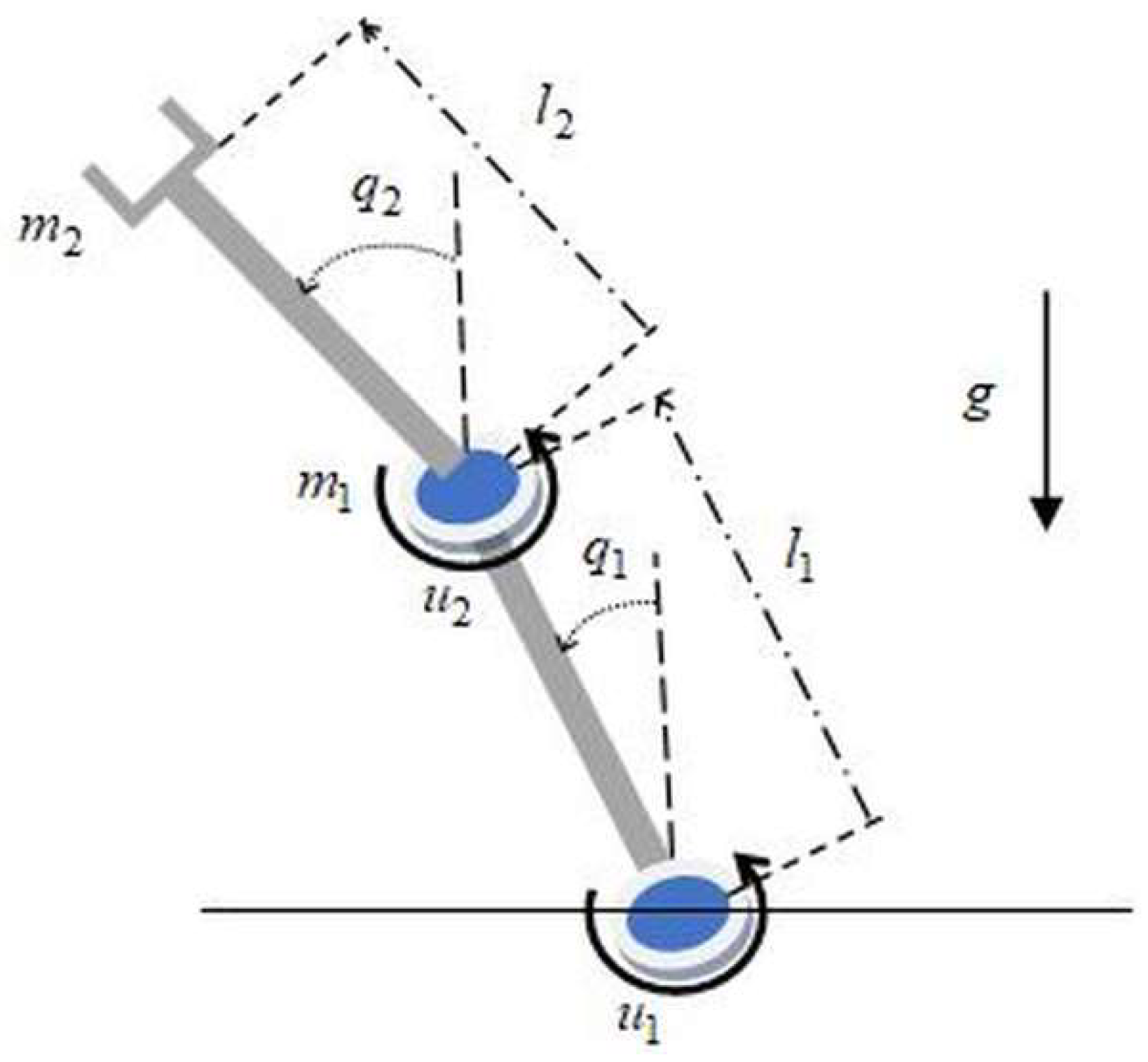
For simplicity, consider a 2-link robot manipulator, as shown in Figure 3, to validate the developed approach of control.

Let $l_1=l_2=0.5\mathrm{m}$ be arm lengths, $m_1=2\mathrm{kg}$ and $m_2=1\mathrm{kg}$ the masses at the end of each joint axe, $g=9.8({\mathrm{m}/\mathrm{s}}^2)$ the gravity acceleration, and $q={\left[\begin{array}{cc}{q}_1& q_2\end{array}\right]}^{}{}^T$ the joint angular position vector.

The robot manipulator is described by the following equation:

$$\ddot{q}=A_0(Q)+B_0(q)u+D$$

(40)

where $A_0(Q)=-J^{-1}(q)\left(C(Q)\dot{q}+G(q)\right)$, $B_0(q)=J^{-1}(q)$ and $D=J^{-1}(q)\left(d-F(\dot{q})\right)$ with, the inertia matrix $J(q)=\left[\begin{array}{cc}{(m_1+m_2)}^{}{l}_1^2& m_2{l}_1{l}_2\left(\sin (q_1)\sin (q_2)+(\cos (q_1)\cos (q_2)\right)\\ m_2{l}_1{l}_2\left(\sin (q_1)\sin (q_2)+(\cos (q_1)\cos (q_2)\right)& m_2{}^{}{l}_2^2\end{array}\right]$, the centripetal Coriolis matrix $C=m_2{l}_1{l}_2\left(\cos (q_1)\sin (q_2)-\sin (q_1)\cos (q_2)\right)\left[\begin{array}{cc}0& -{\dot{q}}_2\\ -{\dot{q}}_1& 0\end{array}\right]$, the gravity vector $G={\left[\begin{array}{cc}-(m_1+m_1)l_{1}g\sin (q_1)& -m_2{l}_{2}g\sin (q_2)\end{array}\right]}^{}{}^T$, the joint torque input vector $u_{}={\left[\begin{array}{cc}{u}_1^{}& u_2^{}\end{array}\right]}^{}{}^T$, the state vector $Q\begin{array}{c}=\end{array}{\left[\begin{array}{cc}{q}^T& {\dot{q}}^T\end{array}\right]}^{}{}^T\in {ℝ}^4$, the disturbance vector $d=\left[\begin{array}{c}{d}_1\\ d_2\end{array}\right]\in {ℝ}^2$, including un-modeled dynamics, unknown payload dynamics, and other unknown perturbations; and, the unknown friction vector $F(\dot{q})=\left[\begin{array}{c}{F}_1({\dot{q}}_1)\\ F_2({\dot{q}}_2)\end{array}\right]\in {ℝ}^2$.

Assume that the robot manipulator system (40) presents time-varying uncertainties on the mass of joints, as follows: $dm(\mathrm{kg})={\left[\begin{array}{cc}d{m}_1& d{m}_2\end{array}\right]}^{}{}^T={\left[\begin{array}{cc}0.2\sin (2t)& 0.4\sin (2t)\end{array}\right]}^{}{}^T$. Therefore, the dynamic Equation (40) can be rewritten as:

$$\ddot{q}=\left(A_0(Q)+\Delta A(Q)\right)+\left(B_0(q)+\Delta B(q)\right)u+\overline{D}$$

(41)

where $A_0(Q)$ and $B_0(q)$ represent the nominal dynamics; $\Delta A(Q)$ and $\Delta B(q)$ represent the parametric variations on the nominal system caused by $dm$; and, $\overline{D}={\left(J(q)+\Delta J(q)\right)}^{-1}\left(d-F(\dot{q})\right)$.

Un-modeled dynamics, unknown payload dynamics, unknown friction force, parametric variations, and other unknown perturbations are represented as:

$$\overline{D}={\left(J(q)+\Delta J(q)\right)}_{}^{-1}\left[\begin{array}{l}0.2\sin ({\dot{q}}_1)+0.8\sin (2t)+0.4q_1+0.2sign({\dot{q}}_1)\\ 0.2\sin ({\dot{q}}_2)+0.8\sin (2t)+0.4q_2+0.2sign({\dot{q}}_2)\end{array}\right]$$

(42)

where $\Delta J(q)$ represents the parametric variations on the inertia matrix $J(q)$.

Set the initial joint angular position vector $q(rad)={\left[\begin{array}{cc}1.2& 0.4\end{array}\right]}^{}{}^T$; the control objective is to maintain the system to track the desired trajectory $q_d={\left[\begin{array}{cc}{q}_{1d}& q_{2d}\end{array}\right]}^{}{}^T={\left[\begin{array}{cc}\sin (t)& \cos (t)\end{array}\right]}^{}{}^T$.

Set the sliding surfaces $s_1={\dot{e}}_1+{\lambda }_1{e}_1$ and $s_2={\dot{e}}_2+{\lambda }_2{e}_2$, where $e_1=q_{1d}^{}-q_1$ and $e_2=q_{2d}^{}-q_2$are the tracking errors.

Assume that $q_1$, $q_2$, ${\dot{q}}_1$, and ${\dot{q}}_2$ belong to $\left[\begin{array}{cc}-\frac{\pi }{2}& \frac{\pi }{2}\end{array}\right]$.

The proposed AIT2-FSMC law is designed as

$$u=\left[\begin{array}{c}{u}_1\\ u_2\end{array}\right]={\left(B_0(q)+\Delta \widehat{B}(q)\right)}^{-1}\left({\ddot{q}}_d-\left(A_0(Q)+\Delta \widehat{A}(Q)\right)+\lambda \dot{e}-{\widehat{u}}_{sl}^{}\right)$$

(43)

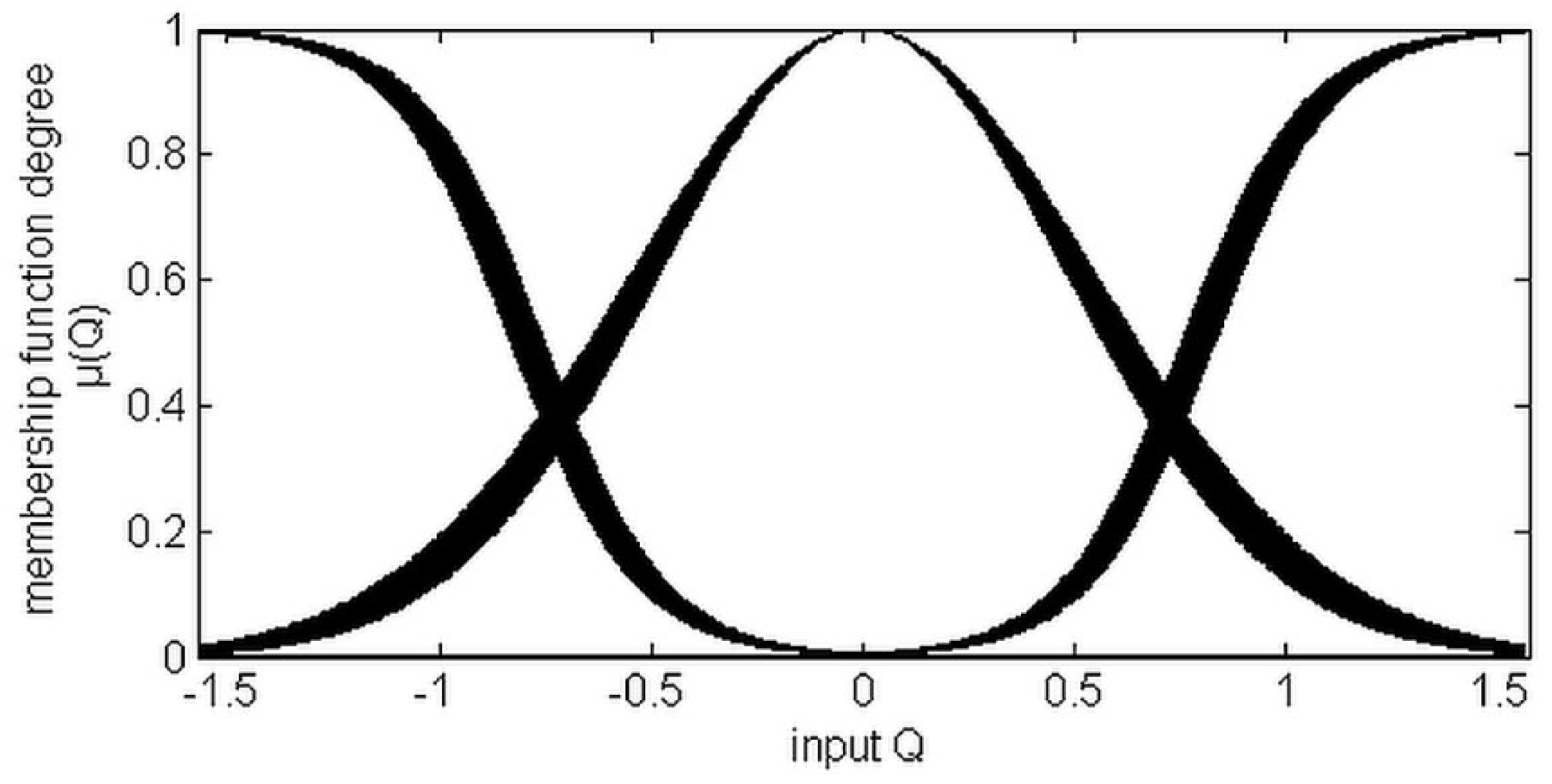
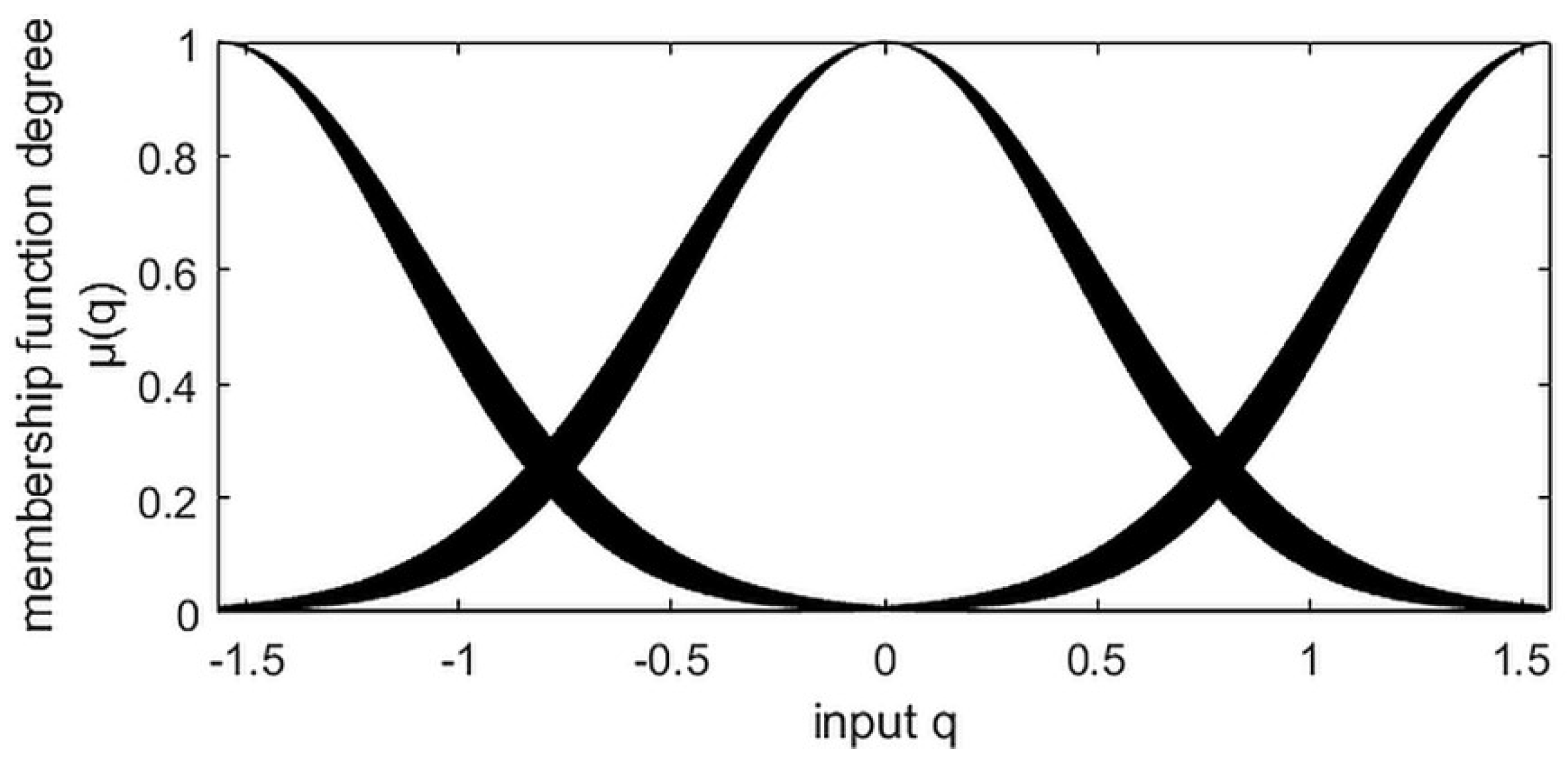
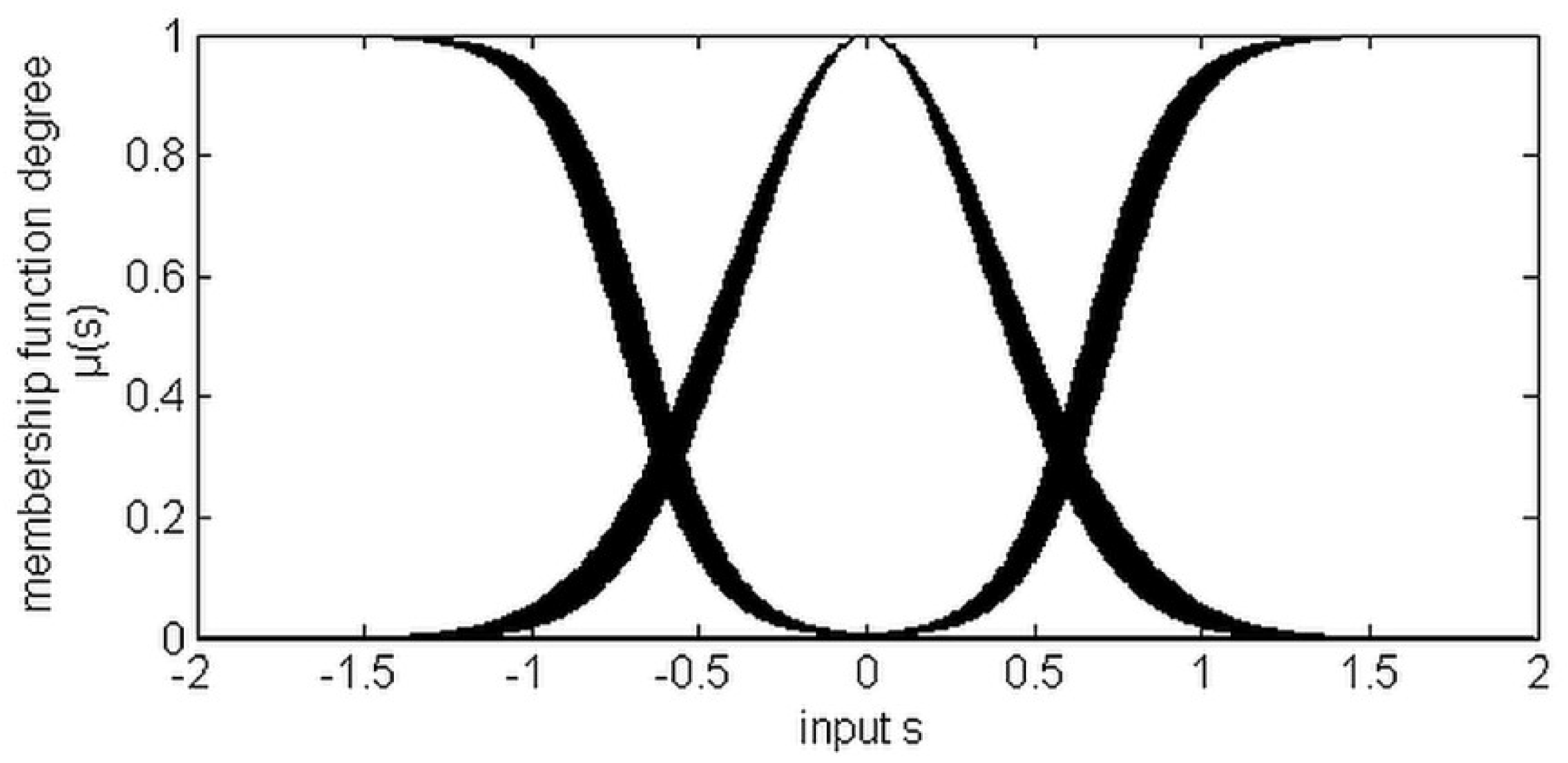
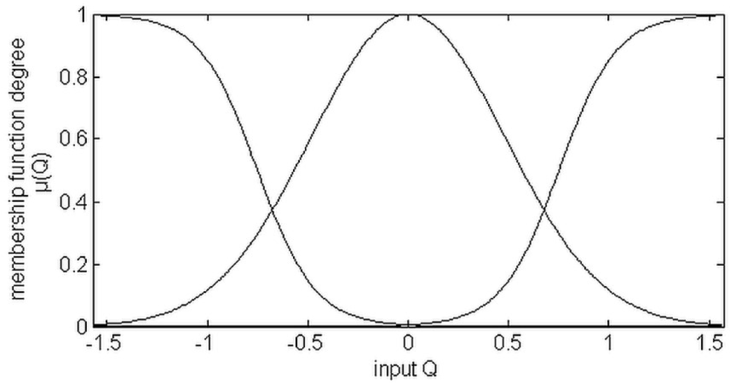
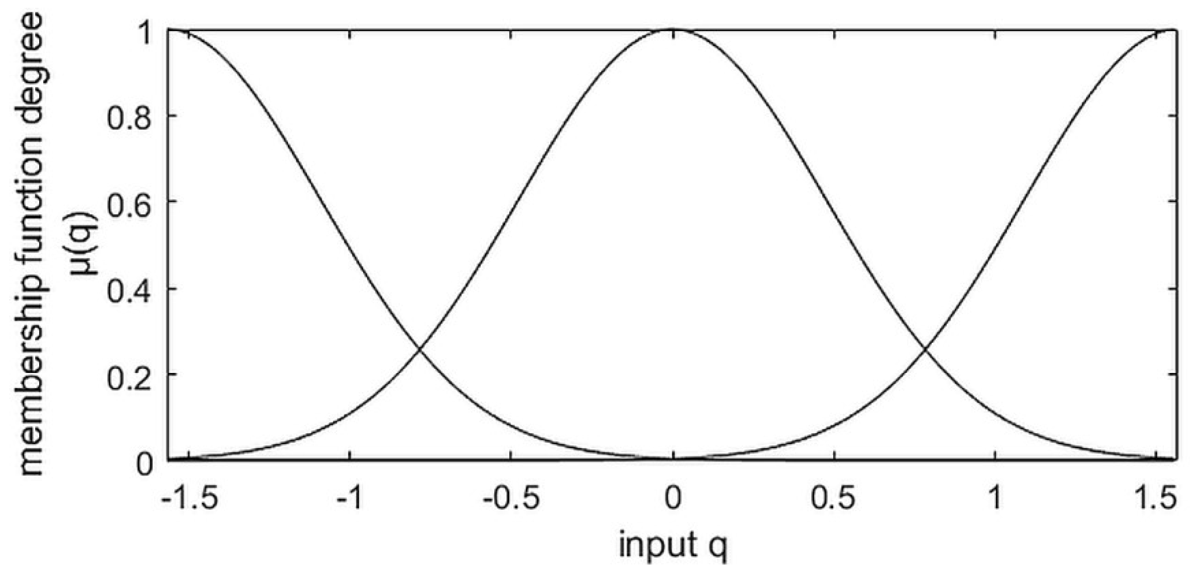
where the AIT2-FLS $\Delta \widehat{A}(Q)$ has four inputs $q_1$, $q_2$, ${\dot{q}}_1$, and ${\dot{q}}_2$, and each of them is defined by three MFs, as represented in Figure 4. The AIT2-FLS $\Delta \widehat{B}(q)$ has two inputs $q_1$ and $q_2$, and each of them is defined by three MFs, as depicted in Figure 5. Likewise, for the AIT2-FLS ${\widehat{u}}_{sl}={\widehat{u}}_{\alpha }+{\widehat{u}}_k+{\widehat{u}}_{\mu }$, three MFs are designed for each of its inputs $s_1$ and $s_2$, as depicted in Figure 6.

To show the effectiveness of the proposed approach of control, a comparison was made with the adaptive fuzzy SOST-SMC algorithm (AFSOST-SMC) that uses AT1-FLSs $\Delta \overline{A}(Q)$ and $\Delta \overline{B}(q)$ to approximate $\Delta A(Q)$ and $\Delta B(q)$, and it uses a SOST-SMC law to handle the approximation errors and unknown disturbances.

The global control law of the AFSOST-SMC approach is given as:

$$V=\left[\begin{array}{c}{V}_1\\ V_2\end{array}\right]={\left(B_0(q)+\Delta \overline{B}(q)\right)}^{-1}\left({\ddot{q}}_d-\left(A_0(Q)+\Delta \overline{A}(Q)\right)+\lambda \dot{e}-u_v^{}\right)$$

(44)

where, $u_v=-\left[\begin{array}{cc}{\alpha }_1& 0\\ 0& {\alpha }_2\end{array}\right]\left[\begin{array}{c}{\displaystyle \underset{0}{\overset{t}{\int }}sign(s_1)dt}\\ {\displaystyle \underset{0}{\overset{t}{\int }}sign(s_2)dt}\end{array}\right]-\left[\begin{array}{cc}{\beta }_1& 0\\ 0& {\beta }_2\end{array}\right]\left[\begin{array}{c}{\left|s_1\right|}^{0.5}\\ {\left|s_2\right|}^{0.5}\end{array}\right]$; ${\alpha }_1$, ${\alpha }_2$, ${\beta }_1$, ${\beta }_2$ are the gains of the control law $u_v$.

The T1-FSs used by $\Delta \overline{A}(Q)$ and $\Delta \overline{B}(q)$ to approximate $\Delta A(Q)$ and $\Delta B(q)$, are depicted in Figure 7 and Figure 8, respectively:

For the constant parameters of the two approaches of control, we take the following values, as shown in the

Table 1. Constant parameters of both control approaches.

Parameters	AIT2-FSMC	AFSOST-SMC
${\lambda }_1$	6	6
${\lambda }_2$	14	14
${\alpha }_1$	-	5
${\alpha }_2$	-	2
${\beta }_1$	-	10
${\beta }_2$	-	12
${\gamma }_a$	800	20
${\gamma }_b$	$0.001$	$0.001$
${\gamma }_{\alpha }$	110	-
${\gamma }_k$	$880$	-
${\gamma }_{\mu }$	24	-
$N_1$	0.1	-
$N_2$	0.1	-

below:

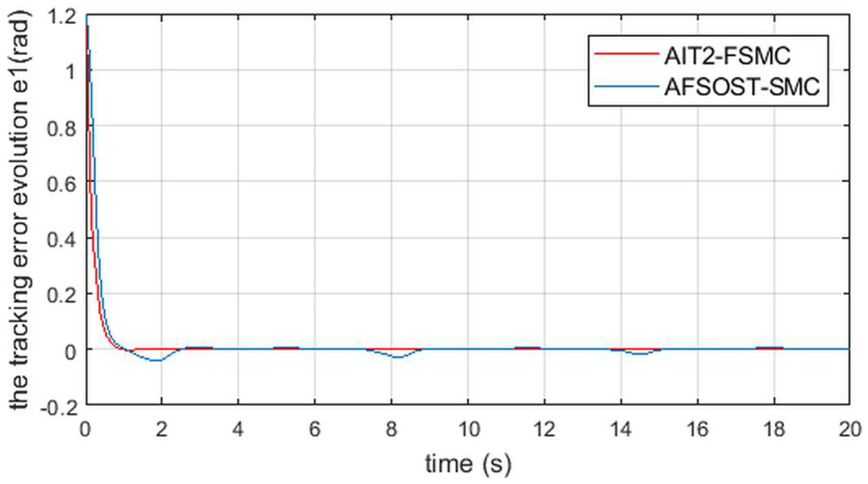
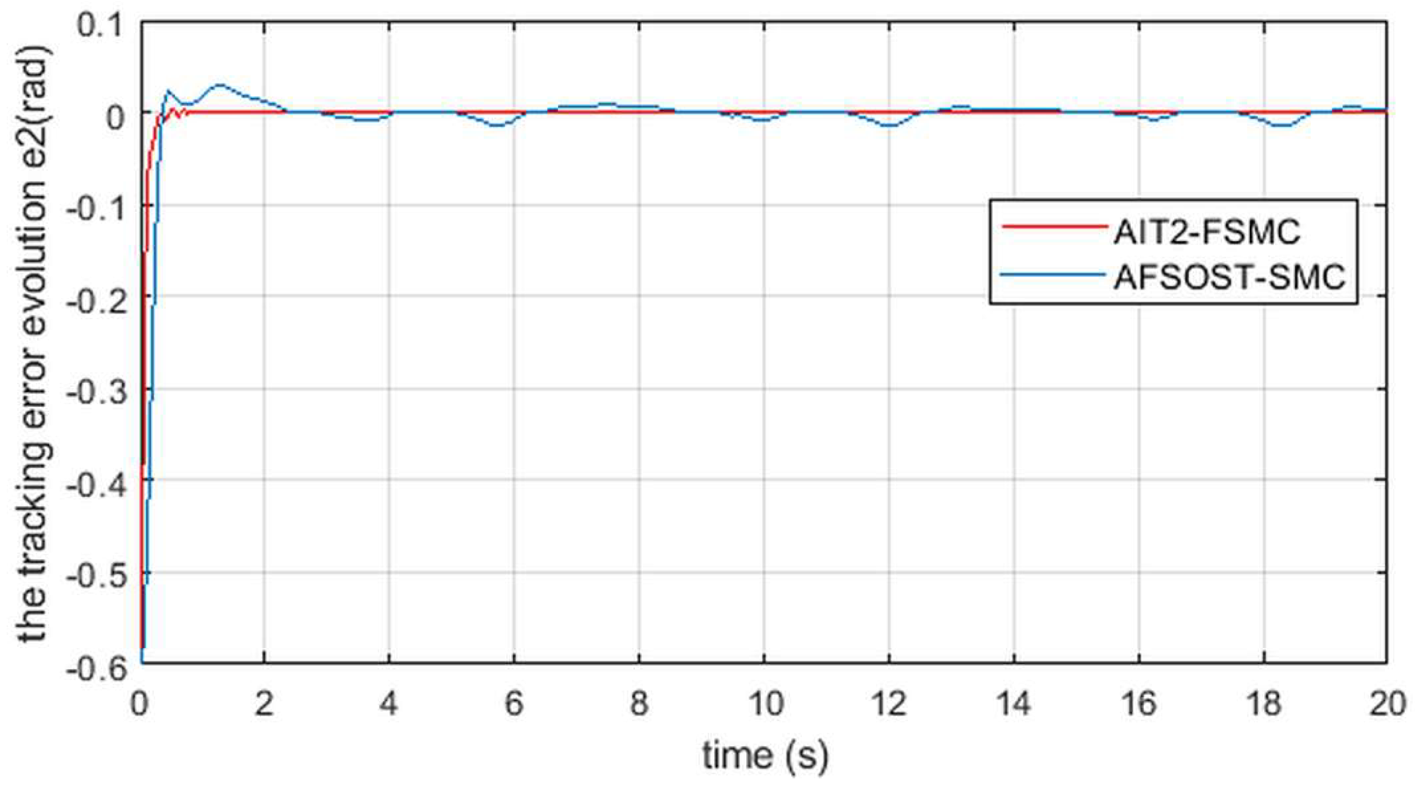
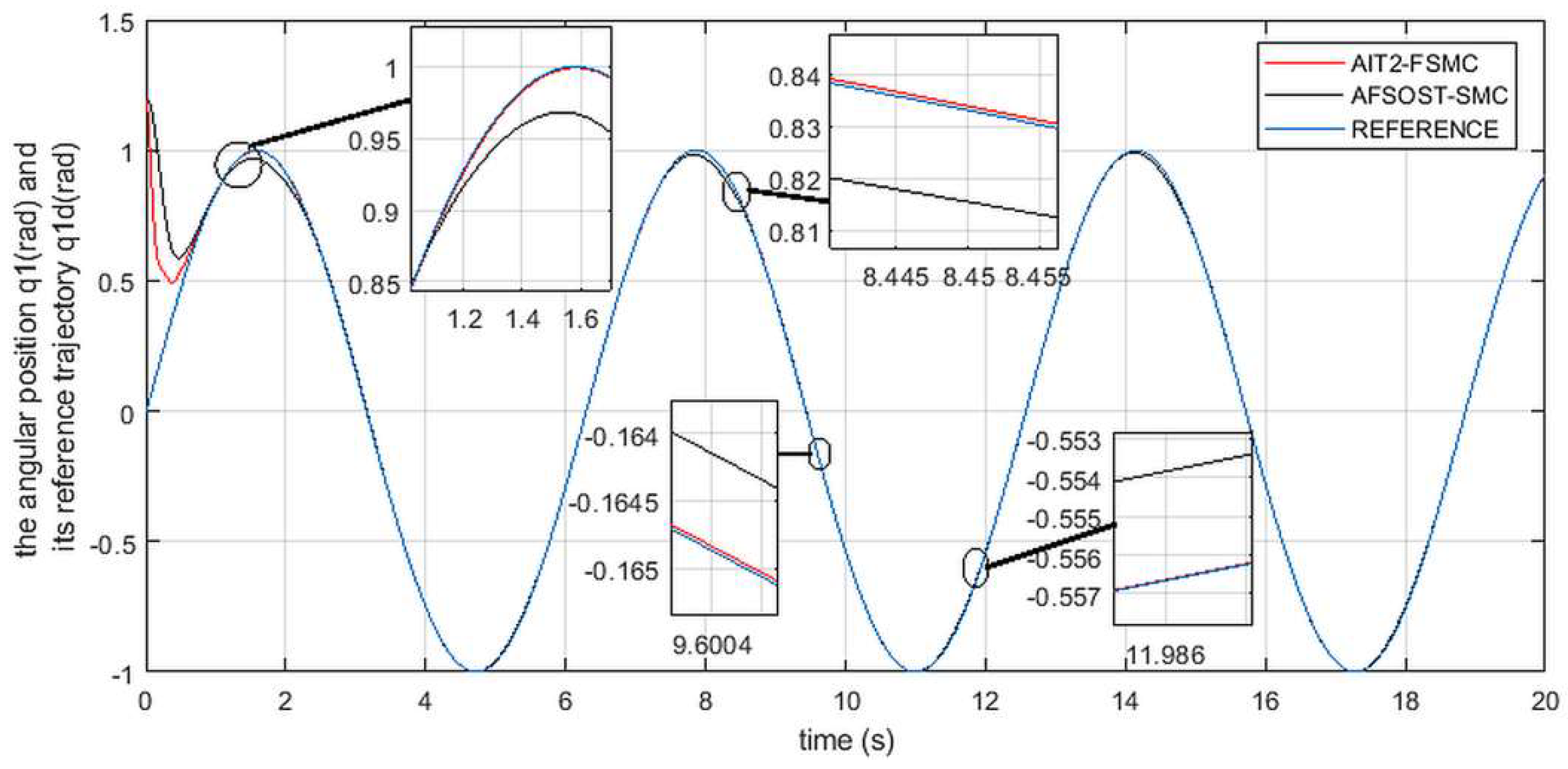
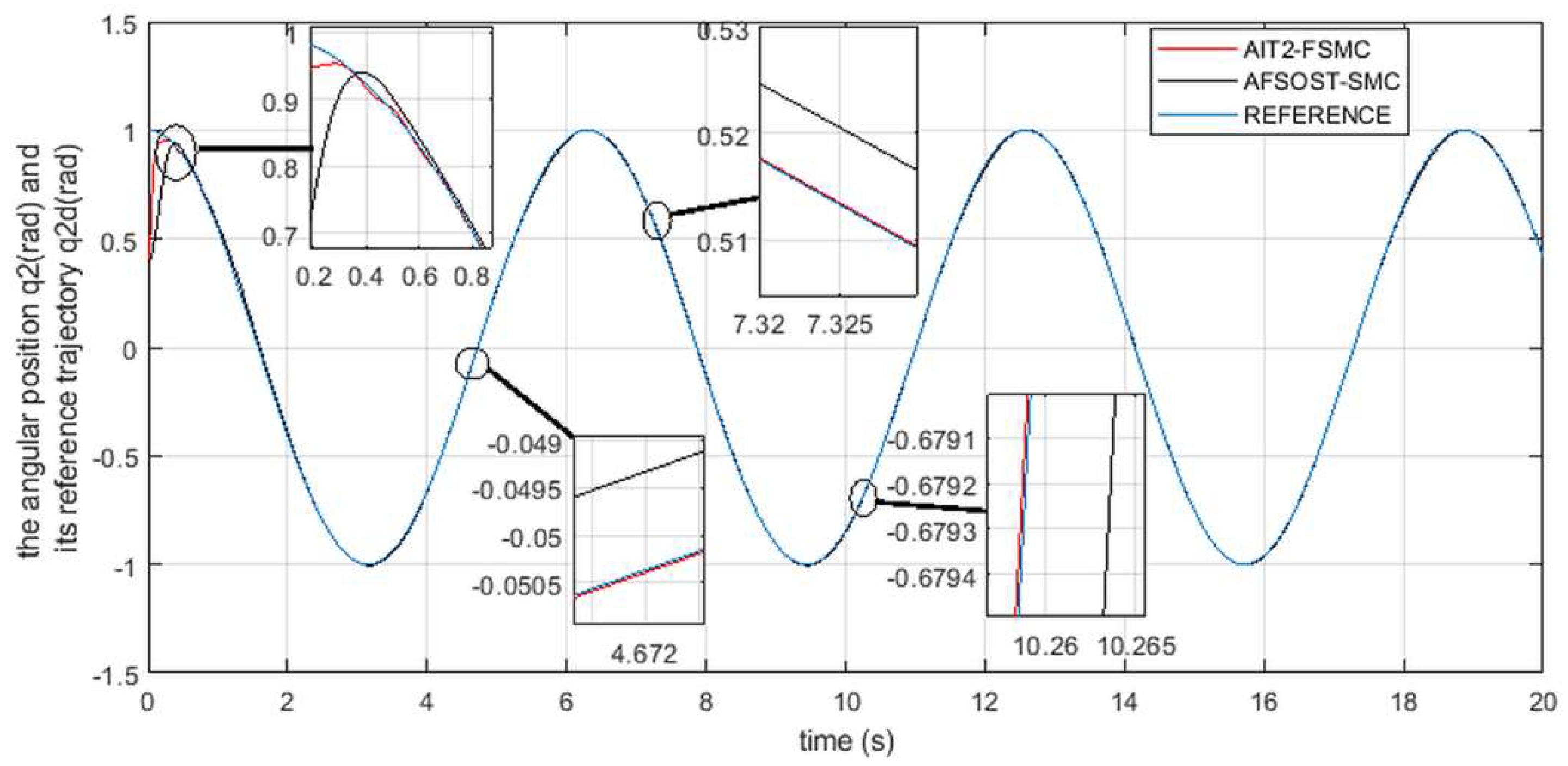
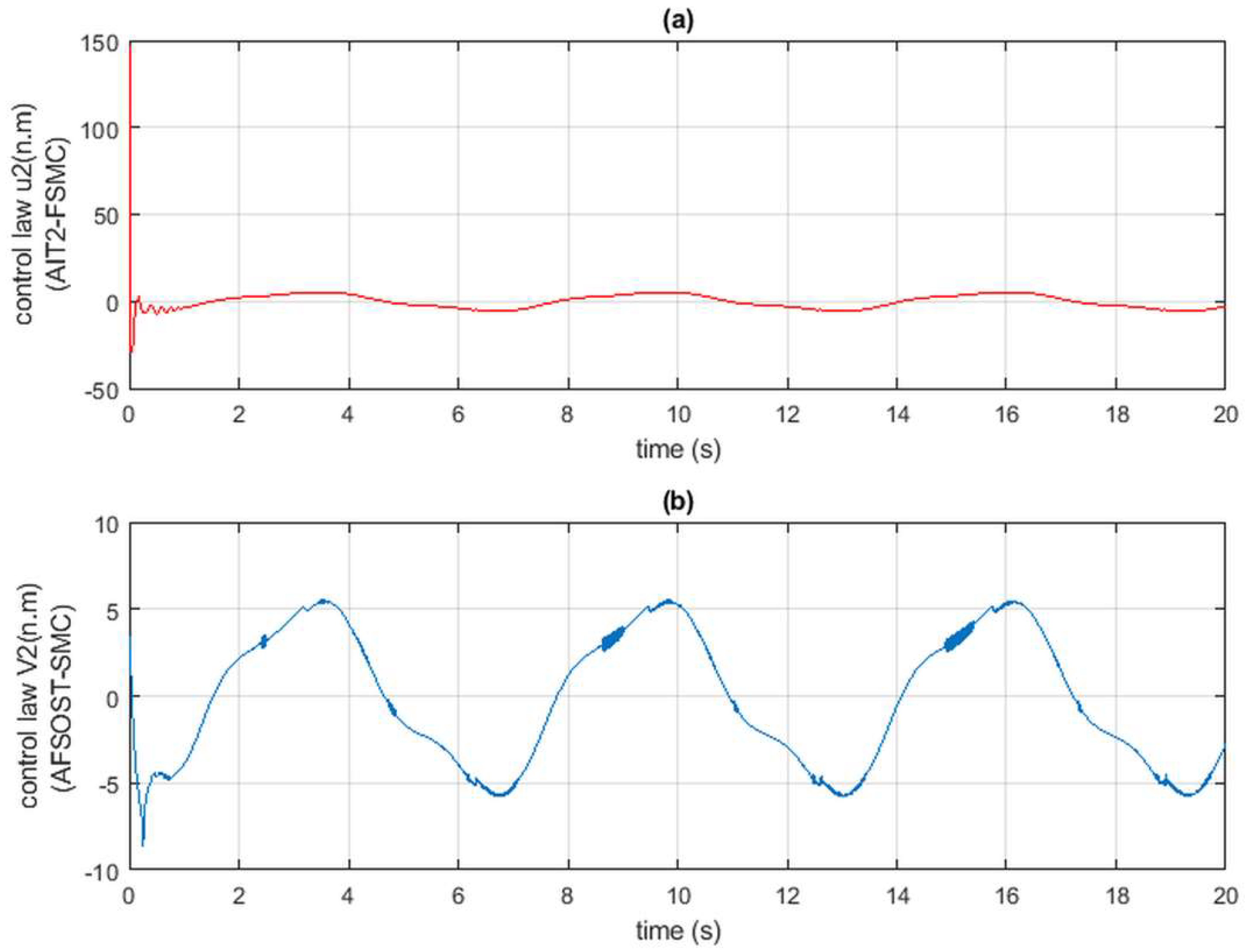
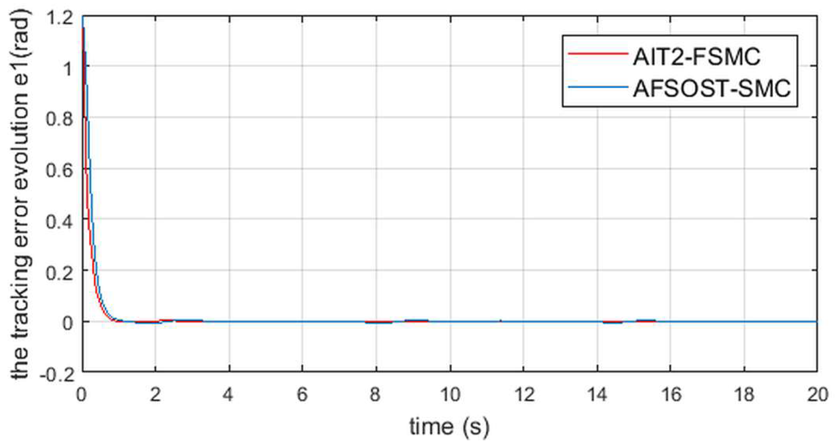
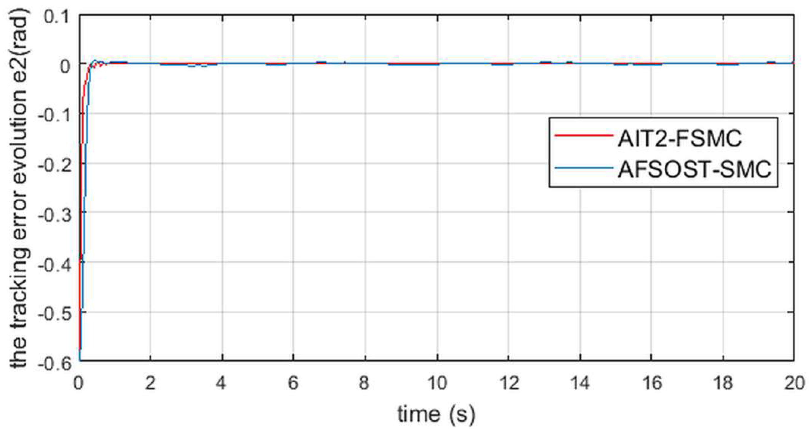
The simulation results are depicted in Figure 9, Figure 10, Figure 11, Figure 12, Figure 13, Figure 14, Figure 15, Figure 16, Figure 17 and Figure 18. They illustrate the comparison between the two control methods, namely the proposed AIT2-FSMC and AFSOST-SMC.

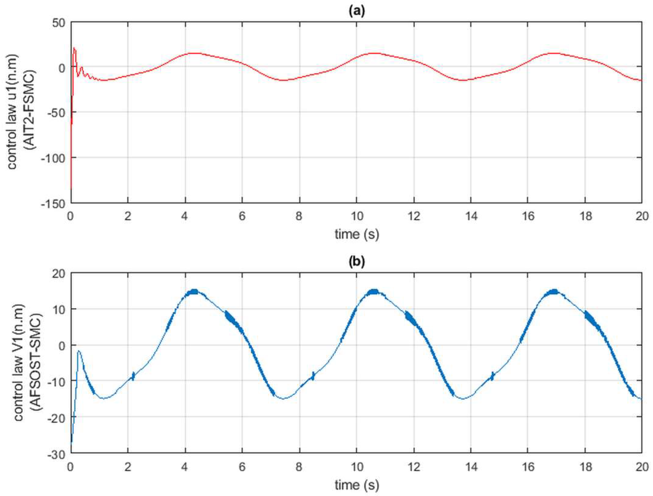
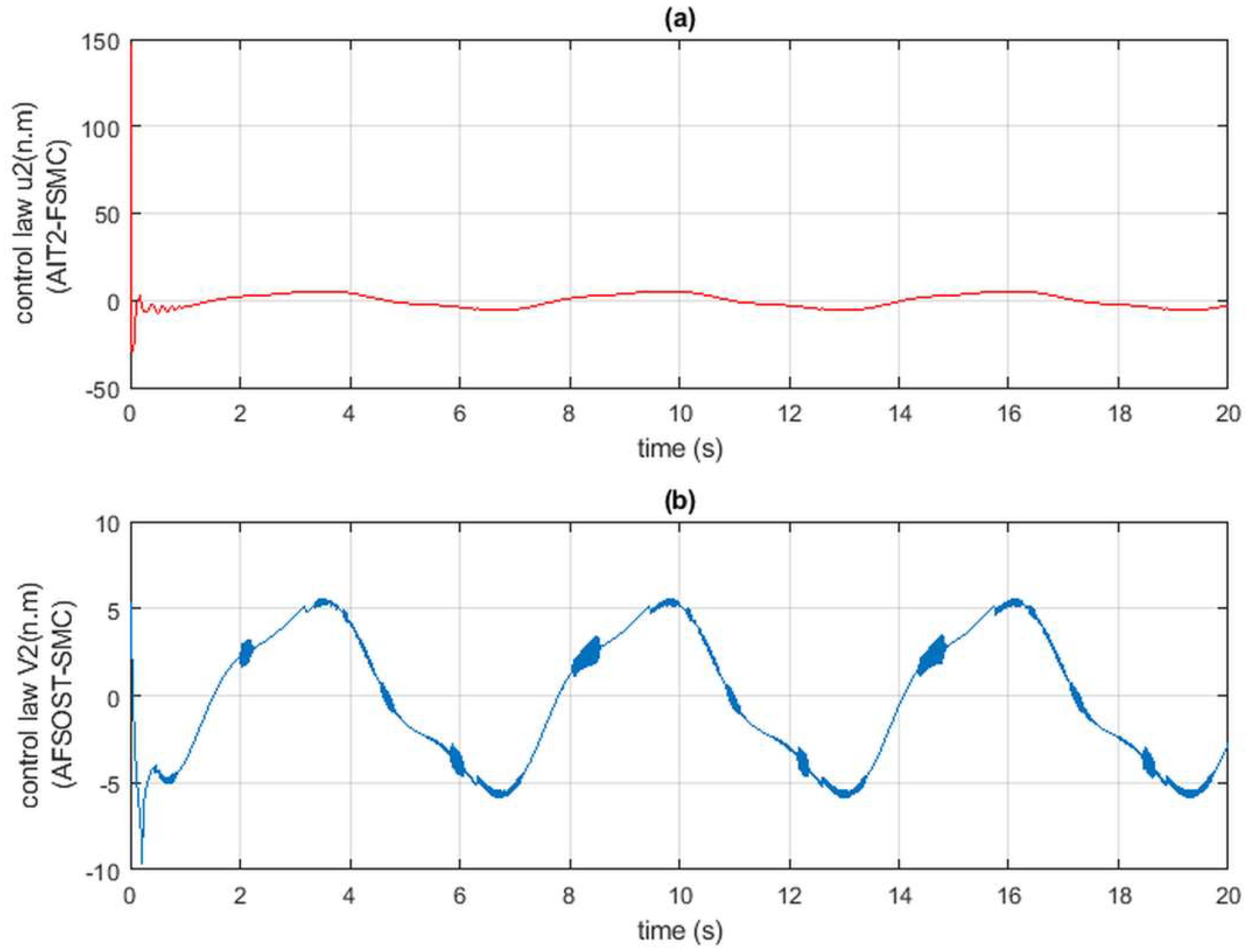
Figure 9 and Figure 10, they show the evolution of the tracking errors. Figure 11 and Figure 12, they depict the robot manipulator angular positions $q_1$ and $q_2$ trajectories, and their desired references $q_{d1}$ and $q_{d2}$, respectively. Figure 13 and Figure 14 they represent the control laws of both control approaches.

The comparison between the AIT2-FSMC and AFSOST-SMC methods shows that the AIT2-FSMC provides better tracking control performance with a smooth control law. This is thinks to the fact that the AIT2-FSMC, firstly, it provides better approximations of the uncertainties $\Delta A(Q)$ and $\Delta B(q)$, and secondly, it rejects the effect of un-modeled dynamics, approximation errors, and other unknown disturbances more efficiently than the AFSOST-SMC.

Figure 15 and Figure 16 below show that the tracking accuracy of the AFSOST-SMC approach is improved when we increase the gains ${\alpha }_1$, ${\alpha }_2$, ${\beta }_1$, and ${\beta }_2$ of the control law $u_v$. However, this implies control inputs with chattering, as shown in Figure 17 and Figure 18. Even with this improvement in accuracy, which generates the chattering in the AFSOST-SMC method, it is concluded that the AIT2-FSMC approach still shows a better tracking accuracy with smooth control inputs.

5. Conclusions

In this paper, we presented a new enhanced tracking control design for n-link robot manipulators in the presence of un-modelled dynamics, unknown payload dynamics, unknown friction force, parametric variations, and other unknown perturbations. Firstly, two AIT2-FLSs are designed to better approximate the parametric uncertainties, then secondly, a new control algorithm, which uses a new designed AIT2-FSMC law, is introduced in order to handle approximation errors and unknown disturbances that affect the robot manipulator systems. In order to overcome the chattering without deteriorating the system robustness, the AIT2-FSMC generates three adaptive control laws to guarantee the best estimation of the optimal smooth control law that ensures the best tracking control performance, despite the uncertainties and disturbances. The closed loop control system is globally asymptotically stable and mathematically proven. The simulation example confirms the effectiveness of the developed control approach in achieving the desired objectives. In the future, we intend to extend the study to cover a wide range of nonlinear systems, such as underactuated nonlinear systems and non affine nonlinear systems.

References

- Purwar, S.; Kar, I.N.; Jha, A.N. Adaptive control of robot manipulators using fuzzy logic systems under actuator constraints. Fuzzy Sets Syst. 2005, 152, 651–664. [Google Scholar] [CrossRef]
- Cuong, P.V.; Nan, W.Y. Adaptive trajectory tracking neural network with robust compensator for robot manipulators. Neural Comput. Appl. 2016, 27, 525–536. [Google Scholar] [CrossRef]
- Gauzman, C.A.C.; Bustos, L.T.A.; Rubio, J.O.M. Analysis and synthesis of global nonlinear H∞ controller for robot manipulators. Math. Probl. Eng. 2015, 2015, 410873. [Google Scholar] [CrossRef]
- Haghighi, S.T.; Piltan, F.; Kim, J.M. Robust composite high-order super-twisting sliding mode control of robot manipulators. Robotics 2018, 7, 13. [Google Scholar] [CrossRef]
- Rubio, J.J.; Pieper, J.; Meda-Campana, J.A.; Aguilar, A.; Rangel, V.I.; Gutierrez, J.G. Modelling and regulation of two mechanical systems. IET Sci. Meas. Technol. 2018. [Google Scholar] [CrossRef]
- Zhang, F. High-speed nonsingular terminal switched sliding mode control of robot manipulators. IEEE/CAA J. Autom. Sin. 2017, 4, 775–781. [Google Scholar] [CrossRef]
- Pan, Y.; Liu, Y.; Xu, B.; Yu, H. Hybrid feedback feedforward: An efficient design of adaptive neural network control. Neural Netw. 2016, 76, 122–134. [Google Scholar] [CrossRef] [PubMed]
- El Kari, A.; Essounbuli, N.; Hamzaoui, A. Commande adaptative floue robuste: Application à la commande en poursuite d’un robot. Phys. Chem. News 2003, 10, 31–38. [Google Scholar]
- Rubio, J.J. Robust feedback linearization for nonlinear processes control. ISA Trans. 2018, 74, 155–164. [Google Scholar] [CrossRef] [PubMed]
- Zi, B.; Sun, H.; Zhu, Z.; Qian, S. The dynamics and sliding mode control of multiple cooperative welding robot manipulators. Int. J. Adv. Robot. Syst. 2012, 9. [Google Scholar] [CrossRef]
- Pan, Y.; Guo, Z.; Li, X.; Yu, H. Output-feedback adaptive neural control of a compliant differential SMA actuator. IEEE Trans. Control Syst. Technol. 2017, 6, 2202–2210. [Google Scholar] [CrossRef]
- Londhe, P.S.; Santhakumar, M.; Patre, B.M.; Waghmare, L.M. Task space control of an autonomous underwater vehicle manipulator system by robust single-input fuzzy logic control sheme. IEEE J. Ocean. Eng. 2017, 42, 13–28. [Google Scholar] [CrossRef]
- Chen, Z.; Li, Z.; Chen, C.L.P. Disturbance observer-based fuzzy control of uncertain MIMO mechanical systems with input nonlinearities and its application to robotic exoskeleton. IEEE Trans. Cybern. 2017, 47, 984–994. [Google Scholar] [CrossRef] [PubMed]
- Fateh, M.M.; Souzanchikashani, M. Indirect adaptive fuzzy control for flexible-joint robot manipulators using voltage control strategy. J. Intell. Fuzzy Syst. 2015, 28, 1451–1459. [Google Scholar] [CrossRef]
- Kayacan, E.; Kayacan, E.; Ramon, H.; Kaynak, O.; Saeys, W. Towards agrobots: Trajectory control of an autonomous tractor using type-2 fuzzy logic controllers. IEEE/ASME Trans. Mech. 2015, 20, 287–298. [Google Scholar] [CrossRef]
- Andreu-Perez, J.; Cao, F.; Yang, G.-Z. A self-adaptive online brain-machine interface of a humanoid robot through a general type-2 fuzzy inference system. IEEE Trans. Fuzzy Syst. 2018, 26, 101–116. [Google Scholar] [CrossRef]
- Chaoui, H.; Guaeaieb, W.; Biglarbegian, M.; Yagoub, M.C.E. Computationally efficient adaptive type-2 fuzzy control of flexible-joint manipulators. Robotics 2013, 2, 66–91. [Google Scholar] [CrossRef]
- Biglarbegian, M.; Melek, W.W.; Mendel, J.M. Design of novel interval type-2 fuzzy controllers for modular and reconfigurable robots: Theory and experiments. IEEE Trans. Ind. Electron. 2011, 58, 1371–1384. [Google Scholar] [CrossRef]
- Castillo, O.; Amador-Angulo, L.; Castro, J.R.; Garcia-Valdez, M. A comparative study of type-1 fuzzy logic systems and generalized type-2 fuzzy logic system in control problems. Inf. Sci. 2016, 354, 257–274. [Google Scholar] [CrossRef]
- Cazarez-Castro, N.R.; Aguilar, L.T.; Castillo, O. Designing type-1 and type-2 fuzzy lyapunov synthesis for nonsmooth mechanical systems. Eng. Appl. Artif. Intell. 2012, 25, 971–979. [Google Scholar] [CrossRef]
- Ding, S.; Huang, X.; Ban, X.; Lu, H.; Zhang, H. Type-2 fuzzy logic for underactuated truss-like robotic finger with comparison of type-1 case1. J. Intell. Fuzzy Syst. 2017, 33, 2047–2057. [Google Scholar] [CrossRef]
- Alonge, F.; Cirrincoine, M.; D’lppolito, F.; Pucci, M.; Sferlazza, A. Robust active disturbance rejection control of induction motor systems based on additional sliding mode component. IEEE Trans. Ind. Electron. 2017, 64, 5608–5621. [Google Scholar] [CrossRef]
- Kim, N.; Park, Y.; Son, J.E.; Shin, S.; Min, B.; Park, H.; Kang, S.; Hur, H.; Ha, M.Y.H.; Lee, M.C. Robust sliding mode of a vapor compression cycle. Int. J. Control Autom. Syst. 2018, 16, 62–78. [Google Scholar] [CrossRef]
- Shah, A.; Huang, D.; Chen, Y.; Kang, X.; Qin, A. Robust sliding mode control of air handling unit for energy efficiency enhancement. Energies 2017, 10, 1815. [Google Scholar] [CrossRef]
- Levant, A. Chattering analysis. IEEE Trans. Autom. Control 2010, 55, 1380–1389. [Google Scholar] [CrossRef]
- Suryawanshi, P.V.; Shendge, P.D.; Phadke, S.B. A boundary layer sliding mode control design for chatter reduction using uncertainty and disturbance estimator. Int. J. Dyn. Control 2016, 4, 456–465. [Google Scholar] [CrossRef]
- Goel, A.; Swarup, A. Chattering free trajectory tracking control of a robotic manipulator using high order sliding mode. Adv. Comput. Comput. Sci. 2017, 553, 753–761. [Google Scholar] [CrossRef]
- Zhang, X.; Yin, C.; Bai, H. Fixed-boundary-layer sliding-mode and variable switching frequency control for a bidirectional DC-DC converter in hybrid energy storage system. Electr. Power Compon. Syst. 2017, 45, 1474–1485. [Google Scholar] [CrossRef]
- Levant, A. Principles of 2-sliding mode design. Automatica 2007, 43, 576–586. [Google Scholar] [CrossRef] [Green Version]
- Zhang, Y.; Li, R.; Xue, T.; Liu, Z.; Yao, Z. An analysis of the stability and chattering reduction of high-order sliding mode tracking control for a hypersonic vehicle. Inf. Sci. 2016, 348, 25–48. [Google Scholar] [CrossRef]
- Mu, K.; Liu, C.; Peng, J. Robust tracking control for robot manipulator via fuzzy logic system and H∞ approaches. J. Control Sci. Eng. 2015, 2015, 459431. [Google Scholar] [CrossRef]
- Chettouh, M.; Toumi, R.; Hamerlin, M. High-order sliding modes for a robot driven by pneumatic artificial rubber muscles. Adv. Robot. 2012, 22, 689–704. [Google Scholar] [CrossRef]
- Jeong, C.-S.; Kim, J.-S.; Han, S.-I. Tracking error constrained super-twisting sliding mode control for robotic systems. Int. J. Control Autom. Syst. 2018, 16, 804–814. [Google Scholar] [CrossRef]
- Nagesh, I.; Edwards, C. A multivariable super-twisting sliding mode approach. Automatica 2014, 50, 984–988. [Google Scholar] [CrossRef] [Green Version]
- Darfa, L.; Benallegue, A.; Fridman, L. Super twisting algorithm for attitude tracking of four rotors UAV. J. Frankl. Inst. 2012, 349, 685–699. [Google Scholar] [CrossRef]
- Levant, A. Sliding order and sliding accuracy in sliding mode control. Int. J. Control 1993, 58, 1247–1263. [Google Scholar] [CrossRef]
- Yen, V.T.; Nan, W.Y.; Cuong, P.V.; Quynh, N.X.; Thich, V.H. Robust adaptive sliding mode control for industrial robot manipulator using fuzzy wavelet neural networks. Int. J. Control Autom. Syst. 2017, 15, 2930–2941. [Google Scholar] [CrossRef]
- Kapoor, N.; Ohri, J. Sliding mode control (SMC) of robot manipulator via intelligent controllers. J. Inst. Eng. Ser. B 2017, 98, 83–98. [Google Scholar] [CrossRef]
- Feng, J.; Gao, Q.; Guan, W.; Huang, X. Fuzzy sliding mode control for erection mechanism with unmodelled dynamics. Autom. J. Control Meas. Electron. Comput. Commun. 2017, 58, 131–140. [Google Scholar] [CrossRef]
- Soltanpour, M.R.; Khooban, M.H.; Soltani, M. Robust fuzzy sliding mode control for tracking the robot manipulator in joint space and in presence of uncertainties. Robotica 2014, 32, 433–446. [Google Scholar] [CrossRef]
- Zi, B.; Sun, H.; Zhang, D. Design, analysis and control of a winding hybrid-driven cable parallel manipulator. Robot. Comput. Integr. Manuf. 2017, 48, 196–208. [Google Scholar] [CrossRef]
- Yu, J.; Liu, J.; Wu, Z.; Fang, H. Depth control of a bioinspired robotic dolphin based on sliding-mode fuzzy control method. IEEE Trans. Ind. Electron. 2018, 65, 2429–2438. [Google Scholar] [CrossRef]
- Hwang, C.-L.; Yang, C.-C.; Huang, J.Y. Path tracking of an autonomous ground vehicle with different payloads by hierarchical improved fuzzy dynamic sliding-mode control. IEEE Trans. Fuzzy Syst. 2018, 26, 899–914. [Google Scholar] [CrossRef]
- John, R.I.B.; Mendel, J.M. Type-2 fuzzy sets made simple. IEEE Trans. Fuzzy Syst. 2002, 10, 117–127. [Google Scholar] [CrossRef] [Green Version]
- Mendel, J.M. Uncertain Rule-Based Fuzzy Logic Systems: Introduction and New Directions; Prentice-Hall PTR: Upper Saddle River, NJ, USA, 2001. [Google Scholar]
- Wu, D.; Mendel, J.M. Enhanced Karnik-Mendel algorithms. IEEE Trans. Fuzzy Syst. 2009, 17, 923–934. [Google Scholar] [CrossRef]
- Slotine, J.J.; Sastry, S.S. Tracking control of non-linear systems using sliding surfaces, with application to robot manipulators. Int. J. Control 2007, 38, 465–492. [Google Scholar] [CrossRef]
Figure 1.
A type-2 fuzzy set.
Figure 2.
A schematic representation of the proposed control approach.
Figure 3.
A 2-link robot manipulator.
Figure 4.
Interval type-2 fuzzy sets used by the AIT2-FLS .
Figure 5.
Figure 6.
Figure 7.
Type-1 fuzzy sets used by the fuzzy system .
Figure 8.
Figure 9.
The tracking error of both control approaches.
Figure 10.
Figure 11.
The angular position of both control approaches, and its reference trajectory .
Figure 12.
Figure 13.
(a) The control law of the control approach AIT2-FSMC; (b) The control law of the control approach AFSOST-SMC.
Figure 14.
Figure 15.
The tracking error of both control approaches, for .
Figure 16.
Figure 17.
(a) The control law of the control approach AIT2-FSMC; (b) The control law of the control approach AFSOST-SMC, for .
Figure 18.