1. EASE-Grid History and Attributes
Defined in the early 1990s as part of the NOAA/NASA Polar Pathfinder Program for gridded, satellite-derived passive microwave brightness temperatures, the Equal-Area SSM/I Earth Grid (
EASE-Grid) was simple to use and understand. The original definition [
1,
2] specified three projections together with the Backus–Gilbert interpolation method used for the SSM/I (Special Sensor Microwave/Imager) Pathfinder data set [
3]. The
EASE-Grid projection and gridding scheme was quickly adopted and used with different interpolation methods by the SMMR, AVHRR and TOVS Polar Pathfinder projects, and has been used in the production of numerous other data sets since then. Over time, the authors realized that the projection and gridding scheme had become so widely used that the SSM/I in the original name was a misnomer, since there was nothing SSM/I-specific about the projection and grid definitions. By 2002, Brodzik and Knowles [
4] decided to retain the acronym but changed the meaning to “Equal-Area
Scalable Earth-Grid”, to emphasize the versatility of applications it enjoyed. Today, the term
EASE-Grid refers to the three original projections and associated gridding scheme, but does not include prescriptions for binning or interpolation methods.
The
EASE-Grid definition [
4] specifies a set of three equal-area projections together with an infinite set of potential grid (spatial resolution and coverage) definitions. The
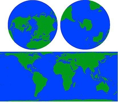
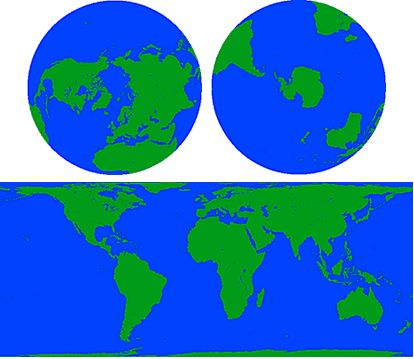
EASE-Grid projections comprise polar aspect Lambert azimuthal equal-area projections (
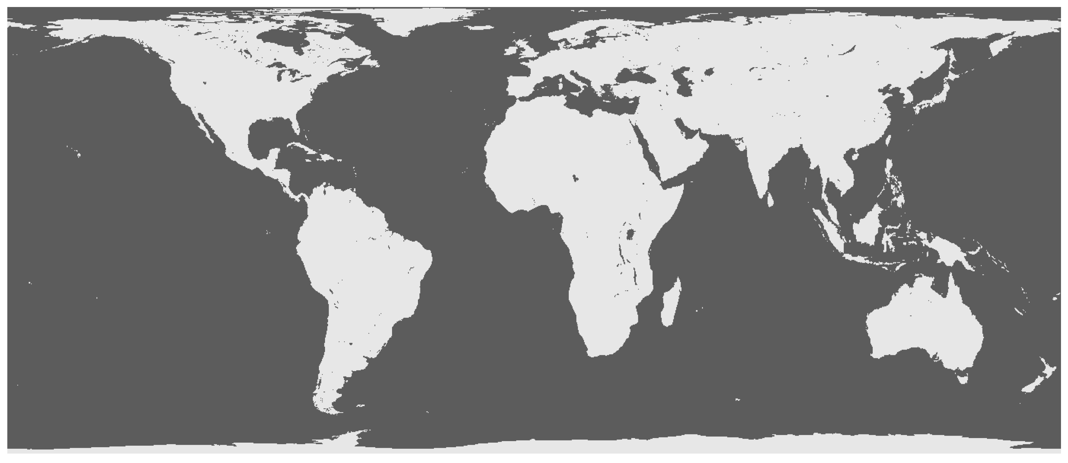
Figure 1) for Northern or Southern Hemisphere, and a cylindrical equal-area projection with standard parallels at ±30°(
Figure 2) for applications in mid- and low-latitude regions.
Figure 1.
Northern and Southern
EASE-Grid projections. See second figure in
Section 2 for zoomed corner subset.
Figure 1.
Northern and Southern
EASE-Grid projections. See second figure in
Section 2 for zoomed corner subset.
The first EASE-Grids, defined for SSM/I gridded brightness temperatures at 25-km resolution, spanned the full Northern and Southern Hemispheres in the azimuthal aspects and the global projection to a latitude of ±86.72°. This poleward extent was inside the data area near the pole for SSM/I, where no data were collected by the sensor due to orbital inclination and the sensor geometry. The grid resolution was chosen to approximate the SSM/I spatial sampling resolution of 25 km. The SSM/I sensor also included one scanning frequency at 85 GHz that was sampled at twice the spatial resolution of the remaining frequencies. Higher-resolution, 12.5-km EASE-Grids were also defined for each projection with the center location of every other 12.5-km cell co-located with the center of a 25-km cell.
A number of data set producers (including [
5,
6,
7,
8,
9,
10]) have adopted the
EASE-Grid format. For equal-area projections, area calculations are accomplished by simply multiplying a constant cell area by the sum of grid cells with particular characteristics. For polar applications, this simple operation is much easier than area calculations on the common alternative polar stereographic grids, where grid cell area is a function of latitude. Data set producers also take advantage of the
EASE-Grid “scalability” feature by defining custom grid resolutions and areal coverages to suit specific applications [
11].
Figure 2.
Cylindrical EASE-Grid projection.
Figure 2.
Cylindrical EASE-Grid projection.
In the years since the original
EASE-Grid definition, other authors have recommended the use of equal-area projections for gridded data sets. The Peters projection (a cylindrical equal-area projection like the one chosen for the cylindrical
EASE-Grid, but with standard parallels at ±45° instead of ±30°) was recommended for ocean-scale oceanographic applications by Krause and Tomczak [
12], who sought the qualities of fidelity of area combined with a rectangular coordinate system. Trischenko
et al. [
13] have adopted a Lambert azimuthal equal-area projection for their MODIS Arctic Circumpolar Mosaic, noting that this choice of projection reduces image distortion and preserves image information content, which they consider an advantage over gridded data in the typical “lat-lon” (Plate-Carrée, or equidistant cylindrical) projection or the MODIS sinusoidal projection.
The original
EASE-Grid was defined as an easier alternative to swath format data in order to support standardized spatial comparisons of geophysical phenomena derived from satellite microwave data [
1]. Over time,
EASE-Grid has been adopted and used by broader communities to produce gridded data sets that include satellite passive microwave brightness temperatures [
3,
8,
14,
15], permafrost land classifications [
5,
16], atmospheric parameters [
6], surface reflectance, albedo and skin temperature [
7], snow and ice products [
10,
17,
18,
19,
20] and soil moisture [
9]. Judging by the variety and number of these data set producers,
EASE-Grid satisfies a need in communities that choose equal-area projections for gridded data sets.
2. EASE-Grid Limitations
EASE-Grid is a popular gridding choice for satellite-derived data sets, especially applications representing geophysical parameters in the polar regions. However, while the original EASE-Grid is easy to learn and easy to adapt to new applications, it suffers from a set of limitations that make its use with current software packages error-prone for users, mapping experts and non-experts alike.
In the following discussion, we use the ISO19111 terminology explained in Section 2.1.2 and
Appendix A of Iliffe and Lott [
21], with some additional notes relevant to issues with the EASE-Grid definition indicated in italics.
An ellipsoid is a closed surface formed by the rotation of an ellipse about its shorter (minor) axis.
A coordinate system (CS) is a set of rules to define how coordinates are assigned to points, usually by means of associated axes.
A coordinate reference system (CRS) is a CS that defines position, scale and orientation of its axes defined with respect to an object, which for our purposes is the Earth.
Geodetic latitude is the angle from the equatorial plane to the perpendicular to the ellipsoid through a given point.
Geodetic longitude is the angle from the prime meridian plane to the meridian plane of a given point.
An ellipsoidal coordinate system (ECS) is a CS specified by geodetic latitude and longitude.
A
geodetic datum defines the relationship of a 2- or 3-dimensional CS to the Earth.
A geodetic datum defines the position of the origin, the scale, and the orientation of the axes of an ECS with respect to a particular Earth ellipsoid. The characteristics of several Earth ellipsoids are included in Table 1.
A geodetic coordinate reference system (GCRS) is an ECS defined for a particular geodetic datum.
A coordinate conversion is a change of coordinates from one CRS to another, in which the CRSs are either based on the same datum or, if they are based on different datums, no algorithm has been applied to transform the coordinates from one datum to the other.
A coordinate transformation is a change of coordinates from one CRS to another in which the CRSs are based on different datums. In this case, a coordinate transformation algorithm is applied to convert the coordinates of one CRS to conform to the datum of the other CRS.
A map projection is a coordinate conversion from an ECS to a plane. A map projection is defined by various projection parameters, including the projection ellipsoid, the ECS coordinates of the projection origin in the plane, the orientation of the projected axes in the plane with respect to the ECS, and other projection-specific parameters.
A projected coordinate reference system (PCRS) is a CRS derived from a GCRS by applying a specified map projection. Note that the projection ellipsoid specified in the map projection may or may not match the datum specified in the GCRS.
The original
EASE-Grid map projections were defined with a spherical Earth model for the projection ellipsoid, namely the International 1924 Authalic Sphere (see
Table 1 and
Appendix B). However, most of the data currently stored in
EASE-Grid are derived from satellite-based sensors, which have WGS 84 as the GCRS datum. Iliffe and Lott [
21] make a distinction between conversions and transformations by pointing out that conversions are defined and are considered to be exact. They point out that coordinate conversions therefore result in no loss of positional accuracy, which was also explained in Brodzik and Knowles [
4] to justify the choice of a spherical Earth model in the original
EASE-Grid map projection definitions.
The decision to use a spherical Earth model for the PCRS projection ellipsoid with data that are referenced to a GCRS datum for a different ellipsoid does not result in loss of positional accuracy during coordinate conversion, as long as software packages consider the PCRS map projection ellipsoid and the GCRS reference datum separately. The distinction must be handled correctly by any software that reprojects
EASE-Grid data: this requires that users understand the software well enough to know when to apply coordinate conversions alone (reprojecting with no change in GCRS reference datum) versus coordinate transformations (reprojecting and changing the GCRS reference datum).
EASE-Grid data users can encounter problems because a number of popular software packages, including ArcGIS, make the assumption that the PCRS map projection ellipsoid and the GCRS reference datum are the same. These applications typically provide no way to specify different values, or suggest applying an inappropriate coordinate transformation instead of the appropriate coordinate conversion [
22]. Without a thorough understanding of how the software is handling conversions and transformations, an unsuspecting user may perform a reprojection of data from
EASE-Grid that erroneously assumes the GCRS reference datum is the 1924 Authalic Sphere, rather than the actual GCRS reference datum, which is the WGS 84 datum.
Table 1.
Characteristics of Earth ellipsoids (Table 2.1, p. 10 in [
21] and
Appendix B) discussed in the text.
Table 1.
Characteristics of Earth ellipsoids (Table 2.1, p. 10 in [21] and Appendix B) discussed in the text.
| Earth Ellipsoids |
|---|
| Name | Equatorial Radius (m) | Flattening | Calculated Polar Radius | Calculated Eccentricity |
|---|
| | a | f | b = a(1 − f ) | e = |
|---|
| International 1924 Ellipsoid | 6 378 388 | 1/297.0 | 6 356 911.946 | 0.081 991 889 979 0 |
| International 1924 Authalic Sphere | 6 371 228 | 0 | 6 371 228 | 0.0 |
| WGS 84 | 6 378 137 | 1/298.257 223 563 | 6 356 752.314 | 0.081 819 190 842 6 |
In the case of the coarser resolution
EASE-Grids (12.5-km or coarser), the consequences of these errors were not drastic (on the order of one or two grid cell locations). However, recent applications of
EASE-Grid, for example, to store data at 500-m resolution, have led to significant errors in reprojection as in
Figure 3.
Furthermore, formats do not always allow for different GCRS reference datums and PCRS projection ellipsoids. The popular GeoTIFF file format standard requires that the PCRS projection ellipsoid be the same as the GCRS reference datum [
23].
EASE-Grid data cannot be legitimately distributed in GeoTIFF format, therefore, without first applying a coordinate conversion (reprojection with no change in GCRS reference datum) to change the projection ellipsoid from the authalic sphere to WGS 84 [
22,
24]. An alternative but awkward approach would be to apply a coordinate transformation to perform the datum shift from WGS 84 to the authalic sphere, but this would change latitude values by as much as 0.19 degrees, or 20 km near ±45° [
25]. For either of these alternatives, the resulting data would be a legitimate GeoTIFF file, but could no longer be designated
EASE-Grid.
Figure 3.
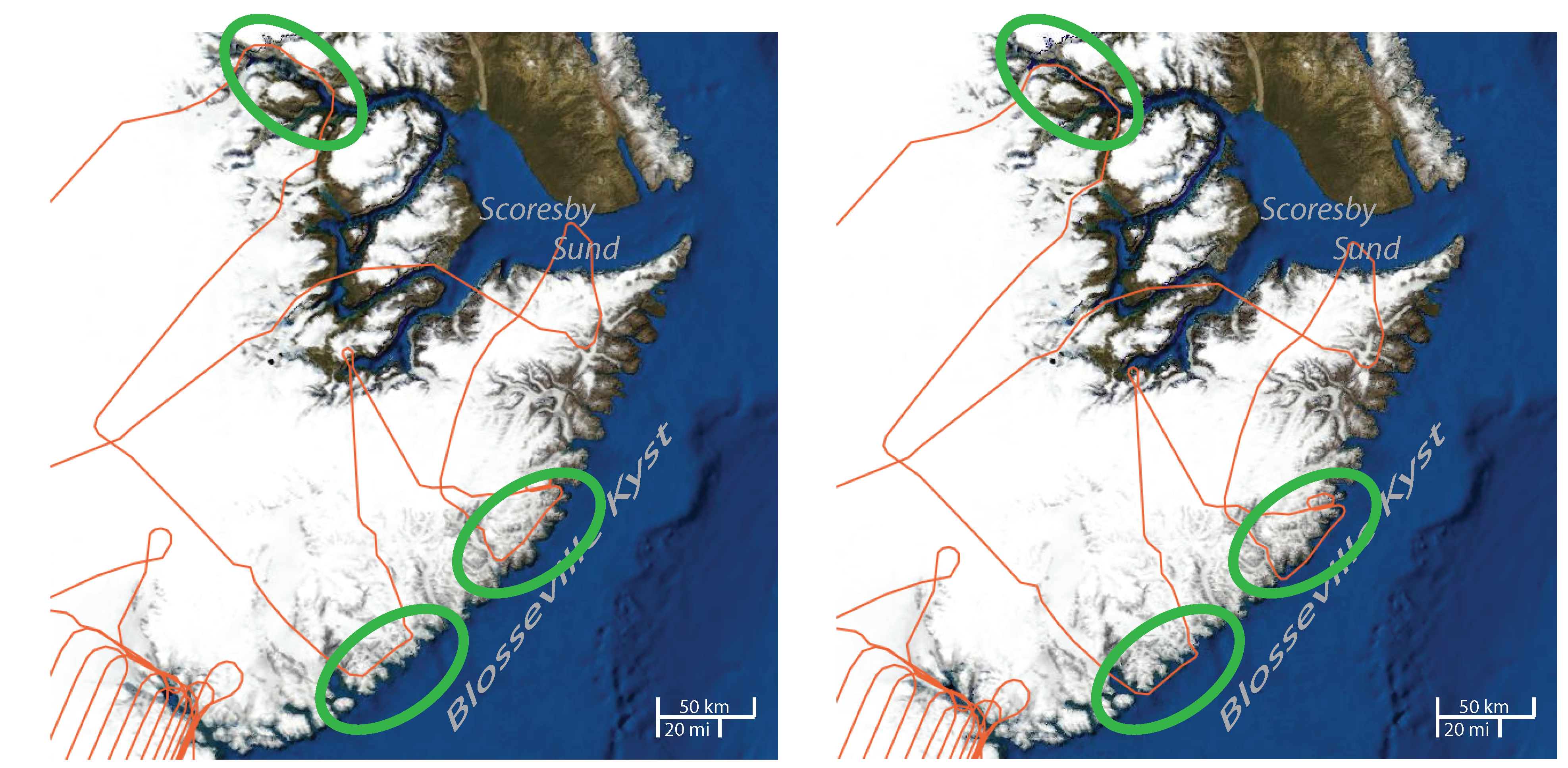
Example of NASA Operation IceBridge flight tracks overlaid on NASA Blue Marble basemap of central eastern Greenland. Blue Marble data are produced in a Plate-Carrée projection referenced to the WGS 84 datum and stored as WMS layers in the original EASE-Grid. The left-hand base map was derived by coordinate transformation into the original EASE-Grid, with an inappropriate datum shift. The right-hand base map was derived correctly by coordinate conversion only (reprojection without the datum shift). The error in the basemap was not identified until the flight manager notified us that the flight track actually traversed down the middle of Daugaard-Jensen Gletscher in the upper Scoresby Sund fjord (top center circle in each image) and that the flightlines parallel to Blosseville Kyst (lower two circles in each image) were performed over sea ice along the coast, not inland.
Figure 3.
Example of NASA Operation IceBridge flight tracks overlaid on NASA Blue Marble basemap of central eastern Greenland. Blue Marble data are produced in a Plate-Carrée projection referenced to the WGS 84 datum and stored as WMS layers in the original EASE-Grid. The left-hand base map was derived by coordinate transformation into the original EASE-Grid, with an inappropriate datum shift. The right-hand base map was derived correctly by coordinate conversion only (reprojection without the datum shift). The error in the basemap was not identified until the flight manager notified us that the flight track actually traversed down the middle of Daugaard-Jensen Gletscher in the upper Scoresby Sund fjord (top center circle in each image) and that the flightlines parallel to Blosseville Kyst (lower two circles in each image) were performed over sea ice along the coast, not inland.
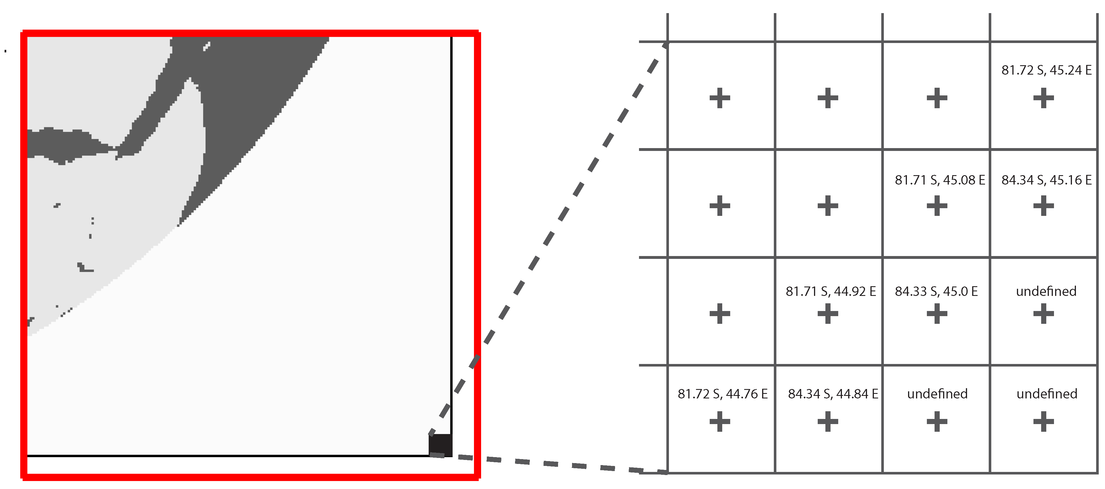
Finally, idiosyncracies at the corners and edges of grids were introduced in the azimuthal
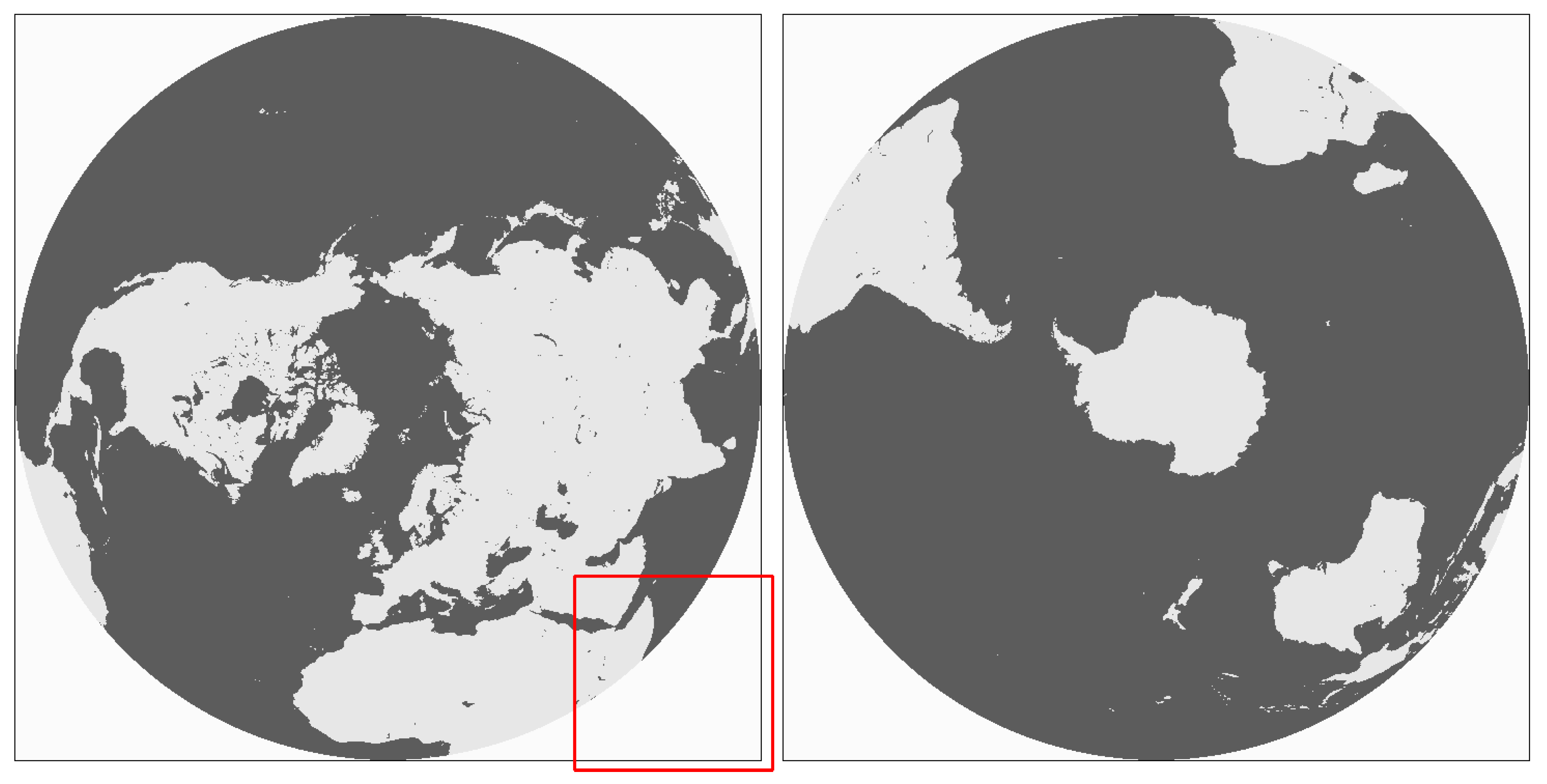
EASE-Grids, due to grid definitions with an odd number of pixels, with the pole located at the center of the center grid cell. Grids at multiples of the original 25-km spatial resolution were defined in a bore-centered fashion. The equator was properly contained (in the mathematical sense of a proper subset) within the extent of the enclosing rectangular grid extent. These choices caused two problems. First, the spatial coverage near each of the four corners of the azimuthal projections extends beyond the opposite pole. While projection coordinates in meters from the projection original are defined at the corners of these grids, the geographic (latitude, longitude) coordinates are undefined (literally “off the Earth”) at locations near the corners of the grid (
Figure 4). Second, the bore-centered relationship forced a partial-cell-sized offset in spatial coverage, so related grids always had different spatial extents. The original justification for the bore-centered relationship was to achieve computational speed in sampling from a finer- to a coarser-resolution grid: no averaging would be required, since each coarse resolution cell was at every other fine-resolution cell location. Over time, this decision has proven difficult to justify. Most users find nested grid cells, that is, four 12.5-km cells nested in a single 25-km cell, easier to conceptualize. Users also consider that grid subsampling rather than averaging is inappropriately discarding data.
Figure 4.
Zoomed area of lower right corner of Northern
EASE-Grid projection in
Figure 1, indicating 25-kilometer corner pixels with undefined (latitude, longitude) coordinates. All corners are symmetric.
Figure 4.
Zoomed area of lower right corner of Northern
EASE-Grid projection in
Figure 1, indicating 25-kilometer corner pixels with undefined (latitude, longitude) coordinates. All corners are symmetric.
While the nominal cell size of the 25 km grids was 25 km × 25 km, the actual cell dimension was slightly larger, 25.06725 km × 25.06725 km, to make the global grid exactly span the equator. Once the scale was chosen for the cylindrical grid, the same scale was used for the azimuthal grids. This decision made documentation simple, with the same scale for all three projections. However, there is no mathematical justification for this decision.
3. EASE-Grid 2.0 Definition
We propose the following new EASE-Grid 2.0 definition to achieve the following goals: (1) make the GCRS reference datum and PCRS projection ellipsoid the same so that formats like GeoTIFF can easily accommodate the data and software packages can easily and properly reproject the data, (2) make nested grid definitions simpler, (3) eliminate undefined geographic coordinates at corners of azimuthal grids (4) decouple scales between cylindrical and azimuthal grids, and (5) select new dimensions that will immediately distinguish data in the EASE-Grid 2.0 format from the original EASE-Grid format.
The EASE-Grid 2.0 definition comprises the same three equal-area projections defined in the original, except that the PCRS projection ellipsoid is WGS 84 rather than the International 1924 Authalic Sphere. Data referenced to the WGS 84 datum and stored in EASE-Grid 2.0 projections can now be formatted directly as GeoTIFF without any reprojection. The likelihood that common software packages will correctly handle reprojection is much higher than with EASE-Grid data.
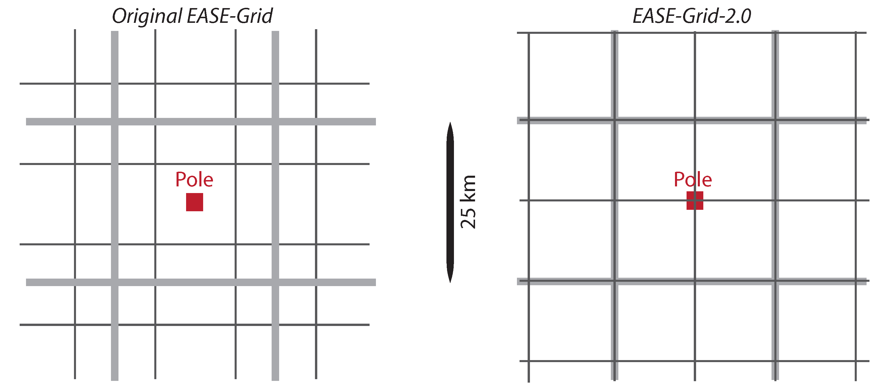
Numbers of rows and columns of the azimuthal grids are even, with the respective pole on the azimuthal grids located at the intersection of the center four grid cells (
Figure 5).
Figure 5.
Relative gridding schemes for representative azimuthal 25 km and 12.5 km original EASE-Grid ((Left), bore-centered) vs. EASE-Grid 2.0 ((Right), nested) cells near the pole.
Figure 5.
Relative gridding schemes for representative azimuthal 25 km and 12.5 km original EASE-Grid ((Left), bore-centered) vs. EASE-Grid 2.0 ((Right), nested) cells near the pole.
The scale of the cylindrical grid will again be determined as the closest value to the desired nominal scale such that an exact number of cells spans the equator; however, corresponding azimuthal grid scales will be exact. For example, the new 25 km cylindrical grid cell size is 25,025.2600081 m, but the new 25 km azimuthal grid cell size is exactly 25,000.0 m.
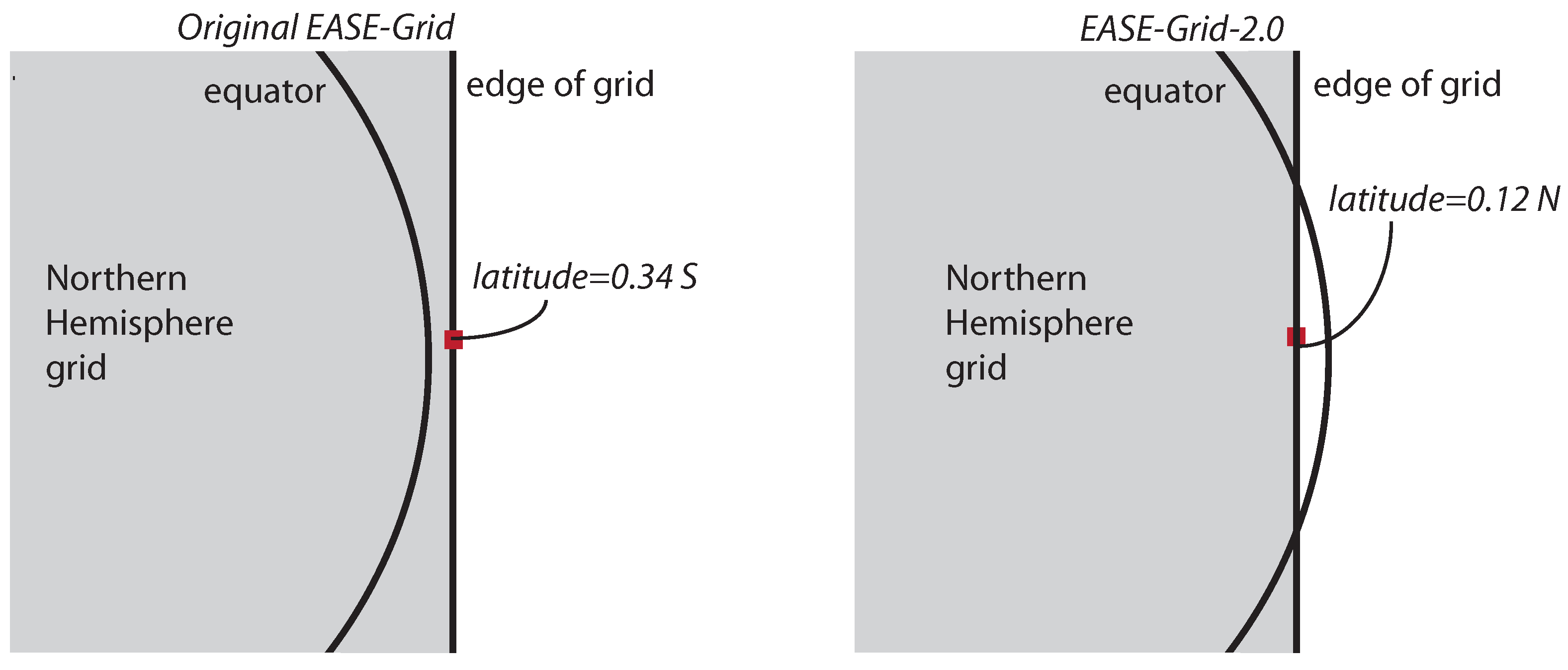
Figure 6.
Relationship of equator to right edge of grid coverage in Northern Hemisphere azimuthal 25-kilometer original EASE-Grid ((Left), equator enclosed within spatial coverage) vs. EASE-Grid 2.0 ((Right), equator slightly outside spatial coverage). Southern Hemisphere grids are defined likewise. Curvature of equator is greatly exaggerated relative to edge of grid.
With the exact scale of 25 km, we chose the number of cells in the new 25 km azimuthal grids to be 720 columns by 720 rows. This positions the equator slightly outside the grid coverage at each of the four array edges (
Figure 6), with a small sector of the hemisphere outside the spatial coverage of the grid. We chose this dimension (1) to avoid the original problem with undefined latitude/longitude values in the grid corners, (2) to promote the many exact multiples and divisors for nested and nesting grids that are possible with the value 720, and (3) to indicate by different grid dimensions alone that the new grids are different from the original
EASE-Grids (the original 25 km azimuthal
EASE-Grid dimensions are 721 columns × 721 rows).


