Article

Prioritizing Areas for Rehabilitation by Monitoring Change in Barangay-Based Vegetation Cover

1
Division of Spatial Information Science, Graduate School of Life and Environmental Sciences, University of Tsukuba, 1-1-1 Tennodai, Tsukuba City, Ibaraki 305-8572, Japan
2
Don Mariano Marcos Memorial State University, Bacnotan 2515 La Union, Philippines
*
Author to whom correspondence should be addressed.
ISPRS Int. J. Geo-Inf. 2012, 1(1), 46-68; https://doi.org/10.3390/ijgi1010046
Submission received: 29 December 2011 / Revised: 1 March 2012 / Accepted: 5 March 2012 / Published: 13 March 2012

Abstract

:
Analysis of spatial and temporal changes of vegetation cover using remote sensing (RS) technology, in conjunction with Geographic Information Systems (GIS), is becoming increasingly important in environmental conservation. The objective of this study was to use RS data and GIS techniques to assess the vegetation cover in 1989 and 2009, in the barangays (smallest administrative units) of the city of San Fernando, La Union, the Philippines, for planning vegetation rehabilitation. Landsat images were used to prepare both the 1989 and 2009 land cover maps, which were then used to detect changes in the vegetation cover for the barangays. In addition to conventional accuracy assessment parameters such as; proportion correct, and standard Kappa index of agreement, two other parameters; quantity, and allocation disagreements were used to assess the accuracy of the land cover classification. Results revealed that there were gains and losses of vegetation cover in most of the barangays, but overall vegetation cover increased by 11% (around 625 ha) based on the original extent of 1989. Those barangays that showed substantial net losses in vegetation cover need to be prioritised for rehabilitation planning. As exemplified in this study, the collection, processing and analysis of relevant RS and GIS information, can facilitate priority-setting in the planning of environmental rehabilitation and conservation by the local government at both city and barangay levels.

Graphical Abstract

1. Introduction

Land use/cover change (LUCC) analysis is a critical component of sustainable land use planning [1,2]. In order to better understand the interactions between human and natural phenomena, timely and accurate detection of change in the earth’s surface features is needed [3]. Furthermore, multi-temporal sets of data are required when monitoring LUCC in order to have effective and accurate evaluations of human impact on the environment [4]. Remote Sensing (RS) has contributed to the fulfilment of this particular requirement by providing much of the necessary data via satellite imagery. Previous studies have highlighted the importance of LUCC for sustainable land use planning in Southeast Asia [5,6]. In the Philippines, biodiversity loss [7], water quality deterioration [8], and natural disasters like flash floods and landslides [9,10,11] have been associated with the loss of vegetation cover. However, the century old ‘theory’ that vegetation cover like forests prevent floods by acting as a giant sponge soaking up water during heavy rains, has been refuted by [12] arguing that there is no scientific evidence linking large scale flooding to deforestation. Nevertheless, it has been stressed that watershed management projects like soil and water conservation and reforestation activities may be beneficial on a local scale, i.e., with a well-developed undergrowth and litter layer, forests may contribute to reducing erosion and sedimentation [12], which have adverse effects on aquatic and reservoir life, potable water quality, irrigation quality and navigation [13].
The Philippines has suffered from a substantial loss in natural vegetation, particularly during the last century. From a forest cover of around 90% of the total area of the country in 1521 [14], this figure has decreased gradually to 62% in 1920, 35% in 1967 and 22% in 1987 through deforestation [15]. As a counter measure, provisions on environmental law were incorporated into the 1987 Philippine Constitution. Specifically, the Constitution states in its declaration of principles and state policies in Article II, Section 16 that; ‘the State shall protect and advance the right of the people to a balanced and healthful ecology in accord with the rhythm and harmony of nature’. Also, Article XII, Section 2 states that; ‘with the exception of agricultural land, all other natural resources shall not be alienated. The exploration, development and utilization of natural resources shall be under the full control and supervision of the State’. These provisions show awareness of the continuing degradation of the country’s environment, which has become a matter of national concern and why over recent years, reforestation projects have been implemented. Based on the latest statistics produced by the Philippines’ Department of Environment and Natural Resources [16], the country’s forest cover increased from 18% in 1995 [15], to 7.168 million ha, or around 24% of the country’s total land area, of which 4.6% is plantation forest. The Philippine Constitution has also been the basis upon which to implement existing forestry and environment-related laws (e.g., the Revised Forestry Code of the Philippines of 1975, and Philippine Environment Code of 1977, amongst others) and to enact new ones (e.g., Executive Order Nos. 23 and 26 of 2011—creating and implementing the National Greening Program, The Philippine Clean Water Act of 2004, The Wildlife Resources Conservation and Protection Act of 2001, and The Philippine Clean Air Act of 1999, amongst others). These policies serve as a legal basis for the barangays, municipalities and cities in their environmental protection and rehabilitation programs.
Some recently published studies relating to LUCC analysis and modelling using medium-resolution satellite images like Landsat images include the following references [17,18,19,20,21,22,23,24,25,26,27,28,29,30,31,32]. Some of them fall under specific research topics like; urban growth analysis and modelling [17,18,21,22,23,30,31], LUCC mapping, analysis and modelling [25,26,27,28,30,31,32,28,30], landscape fragmentation analysis [24,29], and deforestation driving forces analysis and forest conversions forecasting [19,20]. These studies were conducted in various parts of the world. In the LUCC study conducted by [5,20,27,33] in the countries of South and Southeast Asia, most of the selected representative study areas were watershed-based, whilst some others were administrative boundary-based, including national parks. In the Philippines, Lasco and Pulhin [34] analysed the forest land use change and its impact on climate change mitigation for the whole country, whilst Estoque and Murayama [17] monitored the LUCC for Baguio city. In this study, we attempt to extend the monitoring of vegetation cover changes down to the grassroots level, i.e., the smallest administrative unit. Land/vegetation cover changes, more often than not, are within the jurisdiction of the local administrative or political unit. It is here where effective environmental protection and conservation project planning and implementation begin. Republic Act No. 7160 [35], otherwise known as the local government code of the Philippines, states that; ‘as the basic political unit, the barangay serves as the primary planning and implementing unit of government policies, plans, programs, projects, and activities in the community, and as a forum wherein the collective views of the people may be expressed, crystallized and considered, and where disputes may be amicably settled’. At present, each barangay, which is headed by the barangay Captain/Chairman, has defined powers to enhance its existence as an autonomous part of the municipality or city. The local government code of the Philippines [35] provides the barangay executive, legislative and adjudicatory powers, and it is in this context that the barangay is important as a unit of analysis for monitoring changes in vegetation covers.
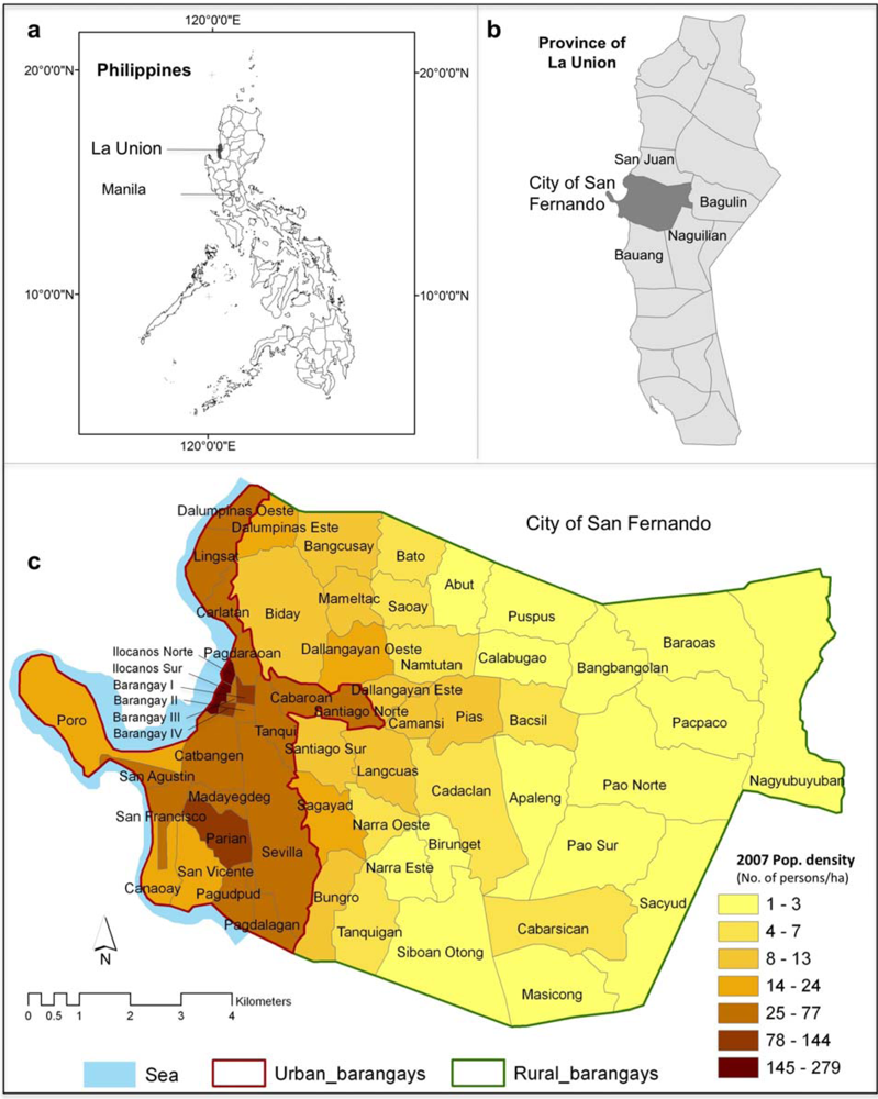
The objective of this study was to assess the vegetation cover for 1989 and 2009 in the barangays of the city of San Fernando, La Union, the Philippines, using medium-resolution RS satellite images and Geographic Information Systems (GIS) techniques for planning vegetation rehabilitation. Having identified the principal changes in vegetation cover between 1989 and 2009 at the barangay level, we discuss the interventions adopted by San Fernando as part of its environmental rehabilitation, protection and conservation agenda.

2. Data and Methods

2.1. Study Area

San Fernando is a coastal city located at 16°37′N latitude and 120°19′E longitude (Figure 1), rising to 500 m above mean sea level [36]. Covering 10,688 ha [37], it is about 60 km from the city of Baguio and 270 km north of Metro Manila. It is bounded by the municipalities of San Juan to the north, Bauang to the south, Bagulin and Naguilian to the east, and the South China Sea to the west.
Figure 1. (a) Map of the Philippines. (b) Map of the Province of La Union. (c) Map of the City of San Fernando showing the 2007 population density per barangay. Note: The National Statistics Office (NSO), the Philippines, classifies the 59 barangays that compose the city into urban barangays (24) and rural barangays (35). Sources: Barangay boundary (2001 Base Map of the City of San Fernando); 2007 Population data [38].
Ijgi 01 00046 g001
San Fernando is a component city of the Province of La Union. According to the National Statistical Coordination Board of the Philippines, a component city is one that does not belong to the categories of highly urbanised and independent component cities. San Fernando, known as the gateway to Ilocandia, is also the centre of the Ilocos region (Region 1), being the seat of national government offices for Region I and the centre of trade, commerce, financial, and educational institutions. The city, comprising 59 barangays, has a population of 114,813 and exhibited an average annual growth rate of about 2% from 1995 to 2007 [38,39,40]. The literacy and employment rates are 97.77% and 94.73%, respectively [37]. The main source of livelihood is agriculture; most of the arable lands are planted with rice, legumes, leafy vegetables, root crops, fruit trees, corn and tobacco [37]. Some people living along the coastline are engaged in fishing activities. The city is also known for its tourist trade. The climate of San Fernando belongs to the Philippine Atmospheric, Geophysical and Astronomical Services Administration (PAGASA)–Climate Type I, being characterised by two pronounced seasons: dry from November to April, and wet for the rest of the year. The temperature may rise above 27 °C, but seldom falls below 26 °C except during the night [41]. The vegetation cover in the city comprises Molave forests and mangrove areas, with a sparse distribution of arboreal species such as rain trees (Samanea saman), and Narra (Pterocarpus spp.) in the city core. Molave forest is a dry, monsoonal forest, which is found only in parts of western Philippines [14]. It occurs in regions where there are distinct wet and dry seasons, each of several months duration. Some of the most important species are Molave (Vitex parviflora), Narra (Pterocarpus spp.), and Ipil (Intsia bijuga), amongst others [42]. Other vegetation includes bushes, shrubs, vines and bamboos in the shrub lands and all of these contribute to the greenery of the city. In general, San Fernando was selected as the study area because it has been active in environmental protection and rehabilitation activities.

2.2. Data Acquisition and Pre-Processing

The two cloud-free images captured during the dry season (8 January 1989 and 9 December 2009) were downloaded from http://glovis.usgs.gov/. The decision was taken to compare vegetation cover during the dry season, so that the effect of rainfall on vegetation phenology would be minimal. Table 1 presents the details of the data used.
In this study, pixels that contained reference features in both time periods were checked to verify that they appeared in the same geographic locations in both images. Although the two images were already orthorectified, upon close examination, a deviation was still observed. Thus, a geometric correction was carried out to minimise the discrepancies using the 1989 image as reference. A total of 26 ground control points and six check points, well distributed across the entire image, were used to geometrically correct the 2009 image in ERDAS IMAGINE® software, following the second order polynomial equations. Both images were resampled to a pixel size of 30 × 30 m, using the nearest neighbour method, in order to maintain the radiometric properties of the original data [31] and this resulted in an RMS error of less than half of a pixel. The images were not radiometrically enhanced before the unsupervised classification was performed to avoid interfering with the original spectral information [43]. The other maps; the previous land use map, topographic map, base map and GeoEye-1 high-resolution satellite images, were all georeferenced based on the two georectified Landsat images with geometric characteristics such as; Projection—UTM, Zone 51N, Spheroid and Datum—WGS 84. The georeferenced base map of San Fernando was digitised on-screen using ArcGIS® software in order to produce a barangay boundary map.
Table 1. Data used and their details.
DataSource/DateScale/ResolutionDescription
Landsat 5 TMNASA Landsat Program/8 January 198930 mNumber of bands: 7
Landsat 7 ETM+NASA Landsat Program/9 December 200930 mNumber of bands: 8
Land use of San FernandoSan Fernando, Philippines/1990s1:20,000Reference image in the classification of the 1989 land cover map
Topographic map of San FernandoNAMRIA, Philippines/19771:50,000Reference image in the classification of the 1989 land cover map
GeoEye-1 satellite images of San FernandoGoogle Earth/15 December 2009; 4 March 2010; 11 April 201050cmReference image in the classification of the 2009 land cover map
Base Map of San FernandoSan Fernando, Philippines/30 May 20011:20,000Reference in digitising the polygon boundary of the city and the barangays
Socio-economic informationSan Fernando, PhilippinesN/AReference in the analysis and discussions

2.3. Land/Vegetation Cover Classification

In the context of this study, vegetation cover includes the commonly used cover classes in land use/cover mapping and studies [17,36,44] such as brushland (shrubs, brushwood, bushes, scrubs, grasses and geophytes) and woodland/forest. In some cases, sparsely distributed trees associated with shrubs/bushes are classified under brushland [17], whilst woodland/forest is further classified into primary, or secondary [20].
Dense vegetation exhibits different spectral characteristics compared with open vegetation. Other land covers like water body and non-vegetated land also have different spectral values. However, a close examination of the satellite images and their spectral information showed that built-up/residential areas and croplands have relatively similar spectral characteristics causing mixed pixels and spectral confusion. Thus, in this study, we only focused on vegetated and non-vegetated land, without further subdividing non-vegetated areas. The four land cover classes; dense vegetation, open vegetation, water body, and non-vegetated land (Table 2 and Figure 2), were adopted for image classification based on; the modified Anderson land use/cover scheme levels I and II [44], the National Mapping and Resource Information Authority (NAMRIA) of the Philippines, and the authors’ a priori knowledge of the study area.
Table 2. Land cover classification scheme for the City of San Fernando.
Land Cover aDescriptions
Open vegetation shrubs, brushwood, bushes, scrubs, grasses, geophytes, and sparsely distributed trees
Dense vegetationwoodland/forest b
Water bodysea, creeks, swamps and other water bodies
Non-vegetated landbuilt-up and residential areas, cropland/agricultural land, bare land and other open areas
a The terms “open” and “dense” vegetation are used in the subsequent discussion; b The forest in the study area is a secondary or second growth forest. There is no primary or virgin forest in the study area.
Figure 2. Visual representation of the land cover classification scheme. The figure covers a part of Barangay Canaoay (see Figure 1). This image is a 2010 GeoEye-1 satellite image used as a reference. Source: Google Earth.
Ijgi 01 00046 g002
We adopted the unsupervised classification method using the Iterative Self-Organizing Data Analysis (ISODATA) algorithm, which uses a minimum distance to assign a pixel to a cluster. We chose this classification method because it clusters the pixels with relatively similar spectral characteristics with a high degree of objectivity [45]. This method is capable of discriminating the four land cover classes adopted in this study. Unsupervised classification using ISODATA uses the original cell value in clustering the pixels with similar spectral characteristics. Since this study focuses on the classification of only a few land cover classes, which can be easily distinguished from each other based on spectral values, ISODATA can be used. Using this method, potential errors due to human limitations on digitising training sites, as in the case of supervised classification, may be avoided. Land cover classification based on the spectral characteristics of the image pixels without training, or forcing the pixels to be in a particular class, is what this study intends, as land cover classes with relatively high spectral confusion (e.g., built, cropland, bare land) were not further distinguished.
In particular, the ISODATA algorithm is affected by the sampling technique and clustering parameters such as the number of clusters [45,46]. A few and also many clusters produce outcomes that are respectively too broad and too detailed, whereby the former may not necessarily reflect reality, whilst the latter requires more computational and processing power and time. In recognition of these considerations, ISODATA was run to generate 20 clusters for both images without assigning a predefined signature set as initial clusters. This number of clusters was determined after several numbers of clusters were empirically assessed in finding the optimum number of clusters for a four-class/category land cover classification. The resultant clusters were assigned to one of the four classes (dense vegetation, open vegetation, water body, and non-vegetated land), by visual interpretation of the original image and reference data (see Table 1) and by using our local knowledge of the study area. Finally, the clusters with the same land cover classes were merged together.

2.4. Accuracy Assessment

A standard overall accuracy for land use/cover maps is set between 85% [44] and 90% [47]. In this study, the accuracy levels of the classified 1989 and 2009 land cover maps were assessed using the georeferenced GeoEye-1 high-resolution satellite images, previous land use map, topographic map and local knowledge of the study area as reference (Table 1). It is assumed that these reference maps are the most accurate maps available for the particular time-periods, so they serve as the basis by which to measure the accuracy of the classification. With a minimum representation threshold of 30 for each land cover category, a total of 250 points were generated for each of the two land cover maps (1989 and 2009) using the stratified random sampling design (unaligned) in ERDAS IMAGINE® software. In this sampling method, the points are stratified based on the distribution of land cover classes [28,31,60]. The possibility of bias is also lessened because it allows the points, or pixels to be randomly selected [48]. Subsequently, the 1989 land cover map was checked with reference to the topographic map and previous land use map, whilst for the 2009 land cover map, the GeoEye-1 high-resolution satellite images were used as reference. The original Landsat image was used as reference for the points, or pixels located in areas covered with clouds in the GeoEye-1 high-resolution satellite images.
The proportion correct and the standard Kappa index of agreement [48,49] have been the most commonly reported parameters for accuracy assessment for a classified land use/cover map. Whilst proportion correct is relatively easy to calculate and understand [50], the standard Kappa index of agreement has been criticised by many authors (e.g., [51,52,53,54]), for giving information that is redundant to proportion correct and misleading for practical decision making [50]. However, proportion correct alone does not give a clear understanding of the errors of the classification. Pontius and Millones [50] proposed the use of two other parameters, or components for accuracy assessment; quantity disagreement, and allocation disagreement. Quantity disagreement is defined as; ‘the amount of difference between the reference map and a comparison map that is due to the less than perfect match in the proportion of the categories (land cover classes)’, whilst allocation disagreement is defined as; ‘the amount of difference between the reference map and a comparison map that is due to less than the optimal match in the spatial allocation of the categories, given the proportions of the categories in the reference and comparison maps [50]. We opted to present all of the four parameters mentioned and we interpreted their respective meanings in relation to the present study.

2.5. Detection of Barangay-Based Vegetation Cover Changes

A post-classification comparison technique using the ‘CROSSTAB’ module in IDRISI® [55] was employed to detect the changes in vegetation cover from 1989 to 2009. By cross-tabulating the 1989 and 2009 land cover maps, we traced the extent of a particular cover class (e.g., how many pixels) that transitioned to other cover classes from 1989 or time 1 (T1), to 2009 or time 2 (T2). The process of cross-tabulating the two images produced a statistical table, which was used to calculate the extent of change of one cover class to another from T1 to T2, and a map that showed the spatial location of the changes, including the non-change areas. The post-classification comparison technique was extended, and a GIS zonal analysis was employed using the 59 barangays in San Fernando as units of analysis. The zonal analysis, which was accomplished using ArcGIS® software, allowed us to summarise the area of each land cover class, and to detect the extent of transition from a particular land cover class to another, in each barangay. The observed changes in vegetation cover for all the 59 barangays in San Fernando, including the ‘gained from’ and ‘lost to’ information, were calculated and the top 15 barangays that gained and lost ‘dense’ vegetation cover were determined. The correlation coefficients between the annual population growth rates (APGR) of these barangays and their respective net gains and losses of ‘dense’ vegetation cover were calculated.

3. Results

3.1. Accuracy Assessment

The results of the accuracy assessment revealed overall classification accuracy levels of 85% and 88%, and kappa statistics of 0.80 and 0.84 for the 1989 and 2009 land cover maps, respectively (Table 3). Based on these parameters (i.e., proportion correct and Kappa), the accuracy levels are within the range reported by some other LUCC studies that used medium-resolution satellite images (i.e., Landsat TM and ETM+) [17,18,19,20,21,22,23,24,25,26,27,28,29,30,31,32] like the ones used in this study. The reported overall accuracies of these studies [17,18,19,20,21,22,23,24,25,26,27,28,29,30,31,32] range from 82% to 99% with an average of 89%. The number of land cover classes ranges from three to nine with an average of six. Those that used an unsupervised classification method [27,31,61] have an overall accuracy ranging from 85% to 90% with an average overall accuracy of 88%, and the number of land cover classes ranges from three to eight with an average of six. In this study, the number of land cover classes (4) influenced the accuracy of the land cover maps, rendering relatively high classification accuracy.
Table 3. Error matrix of the land cover maps derived from Landsat images.
(a) 1989
Classified Data Reference Data Classified TotalsProducer’s Accuracy (%)User’s Accuracy (%)
OpenDenseWater BodyNon-Vegetated Land
Open54606667282
Dense115510678982
Water body00282309793
Non-vegetated land101076879087
Reference totals75622984
Overall classification accuracy = 85%, Overall kappa statistics = 0.80
(b) 2009
Classified DataReference Data Classified TotalsProducer’s Accuracy (%)User’s Accuracy (%)
OpenDenseWater BodyNon-Vegetated Land
Open60402667691
Dense136401789382
Water body00291309797
Non-vegetated land61168769489
Reference totals79693072250
Overall classification accuracy = 88%, Overall kappa statistics = 0.84
Figure 3 presents the details of the allocation and quantity disagreements including the commission, agreement and omission for each land cover class. Allocation disagreement ‘is always an even number of pixels because allocation disagreement always occurs in pairs of misallocated pixels’ [50]. A single pair consists of one pixel of omission for a particular land cover class and one pixel of commission for the same class. An omission pixel is defined as a pixel for a particular land cover class that appears on the reference map, but not on the comparison map (e.g., the pixel is ‘dense’ vegetation in the reference map, but not in the comparison map). A commission pixel is the opposite; where a pixel for a particular land cover class appears on the comparison map and not on the reference map. In calculating the omission and commission, including the agreement for each land cover class relative to the whole study area, Table 3, which contains the sample matrix, had to be converted into a population matrix in order to compute the unbiased summary statistics [50]. The results show that the ‘open’ vegetation cover class had the highest omissions of 9% and 8% in 1989 and 2009, respectively (Figure 3(a,b)). This class had the same commission of 5% with the ‘dense’ vegetation cover and ‘non-vegetated’ land classes in 1989, whilst in 2009 the ‘dense’ vegetation cover class had the highest commission of 6%. In terms of agreement, the ‘non-vegetated’ land class had the highest with 34% and 28% in 1989 and 2009. The ‘dense’ vegetation cover class had an agreement of 23% and 27%, whilst the ‘open’ vegetation cover class had an agreement of 22% and 25% in 1989 and 2009. Thus, the results show that the proportion correct of the ‘non-vegetated’ land class to the whole study area, was relatively lower in 2009 than in 1989, whilst the proportion correct of the ‘dense’ and ‘open’ vegetation cover classes were relatively higher in 2009, compared with 1989. Furthermore, the results revealed that the relative ranking of Kappa is similar to the relative ranking of proportion correct of the two matrices, which means that here, as in other studies (e.g., [17,18,20,22,26,32]), the Kappa indices express information that is superfluous to proportion correct.
The separation of the overall disagreement into components of quantity and allocation, revealed a 4% and 6% quantity disagreement (out of 15% and 12% overall disagreement relative to the whole study area) for the 1989 and 2009 land cover maps, respectively (Figure 3(c,d)), and this allowed some degree of confidence in proceeding with the change detection analysis. This is important because the main purpose of this study focuses on the detection of the net quantity of land cover change between two-time periods, in which allocation disagreement is less important than quantity disagreement [50].
Figure 3. Accuracy assessment. (a) 1989 commission, agreement and omission; (b) 2009 commission, agreement and omission; (c) 1989 allocation and quantity disagreements; and (d) 2009 allocation and quantity disagreements
Ijgi 01 00046 g003

3.2. Land Cover of the City of San Fernando

The source RS satellite images are shown as true colour composites in Figure 4(a) and Figure 5(a). Figure 4(b) and Figure 5(b) show the classified land cover maps of San Fernando for 1989 and 2009, respectively. Table 4 summarises the generated statistics of the different land cover classes and their respective changes from 1989 to 2009. The results showed that the vegetated area of the city was about 54%, whilst the non-vegetated area was about 46% in 1989. Of the vegetated area, 27% was ‘dense’ and 27% was ‘open’ vegetation cover. Of the non-vegetated areas in 1989, 39% was ‘non-vegetated land’, which included built-up and residential areas, cropland/agricultural land, bare land and other open areas, whilst the remaining 7% comprised bodies of water. In 2009, the vegetated area made up 60% of the city, this being broken down into ‘dense’ (33%) and ‘open’ (27%) classifications. The non-vegetated area made up about 40%, of which 32% was ‘non-vegetated land’, with water bodies making up the remaining 8%. Therefore, over a period of 20 years, between 1989 and 2009, the vegetated area in the city increased by about 6% of the whole landscape, or 11% (625 ha) of its original extent in 1989, matched by a corresponding decrease in the non-vegetated area. Of this increase in vegetated area from 1989 to 2009, most (594 out of 625 ha, representing 20% increase of the original area) can be attributed to the increase in ‘dense’ vegetation cover.
The major conversions that occurred on the vegetation cover are given in Figure 6 and Table 5. The results revealed that of the 1,333 ha (gross gain) that transitioned to ‘dense’ vegetation cover; 76.1% was from ‘open’ vegetation cover, 23.8% was from ’non-vegetated land’, and the remaining 0.1% was from water bodies. In the case of the 1,650 ha (gross gain) newly formed ‘open’ vegetation cover; 66.0% was from ‘non-vegetated land’, 33.8% was from ‘dense’ vegetation cover, and the remaining 0.2% was from water bodies.
Hence, whilst ‘dense’ vegetation cover had a gross gain of over a thousand hectares during the transition process it ended up with a net gain of around 600 ha, because some erstwhile ‘dense’ vegetation was lost over this period. In fact, of the total loss of 739 ha; 75.5% was due to conversion to ‘open’ vegetation, 21.5% was lost to ‘non-vegetated land’, and the remaining was lost to water bodies. In the case of the ‘open’ vegetation cover, the results show that whilst it had a relatively high gross gain (1,650 ha) during the process, it ended up with a net gain of around 31 ha. Of the 1,619 ha loss; 62.6% was due to conversion to ‘dense’ vegetation cover (a beneficial development), 36.9% was due to conversion to ‘non-vegetated land’, and the remaining was lost to water bodies.
The change detection analysis revealed that the rate of ‘dense’ vegetation cover loss from 1989 to 2009 was 1.2% per year (36 ha/year), whilst the rate of ‘dense’ vegetation cover gain was 2.3% per year (67 ha/year), giving a net conversion rate to ‘dense’ vegetation cover of around 1.1% per year (30 ha/year) (Table 4 and Table 5). In comparison with other studies that have used medium-resolution RS satellite images, the rate of ‘dense’ vegetation cover loss in San Fernando is much lower than the rate of forest cover loss in the rapidly growing city of Baguio in the Philippines, which was around 3% per year, or 75 ha/year based on the net change from 1988 to 2009 [17]. In County Centre in Pennsylvania, the rate of forest loss at county level from 1993 to 2000 was 0.07% per year (140 ha/year), whilst the rate of forest gain was around 0.12% per year (248 ha/year), giving a net conversion rate to forest of 0.05% per year (109 ha/year) [23]. In Lao PDR, the rate of “current forest” loss from 1993 to 2007 was 2.4% per year (437,400 ha/year), whilst the rate of “current forest” gain was 0.7% per year (129,800 ha/year), giving a net conversion rate from “current forest” of 1.7% per year (307,600 ha/year) [61]. Based on the net change, the rate of primary forest loss in Tam Dao National Park in Vietnam from 1993 to 2007 was 2.4% per year (912 ha/year) [20], whilst the rate of forest loss in Kathmandu valley in Nepal from 1978 to 2000 was around 1% per year (137 ha/year) [24]. Also based on the net change, the rate of conversion to dense forest in the Birahi Ganga sub-watershed of the Garhwal Himalaya in India, from 1976 to 2005 was about 0.1% per year (2 ha/year) [56]. Thus, in comparison with other studies that have used medium-resolution RS satellite images, this study shows that the rate of ‘dense’ vegetation cover loss in San Fernando is within the range of other reported rates. However, although it has a relatively higher percentage rate per year than the others, it has the lowest rate in terms of extent (ha/year). Moreover, although it has the highest percentage rate of gain per year of ‘dense’ vegetation cover, the rate in terms of extent (ha/year) is in the mid-range.
Figure 4. (a) The 1989 Landsat image displayed in its “true colour” composite (RGB:321). (b) The 1989 classified land cover map of the City of San Fernando, La Union, Philippines. Note: See Table 2 for the detailed descriptions of the land cover classes.
Ijgi 01 00046 g004
Figure 5. (a) The 2009 Landsat image displayed in its “true colour” composite (RGB:321). (b) The 2009 classified land cover map of the City of San Fernando, La Union, Philippines. Note: See Table 2 for the detailed descriptions of the land cover classes.
Ijgi 01 00046 g005
Table 4. Statistics of the land cover classes in the City of San Fernando.
Land cover aLand Cover Statistics (ha)Gain/Loss (ha)
198920091989–2009
Open2,8152,84631
Dense2,8993,493594
Water body759866107
Non-vegetated land4,0863,354−732
Total b10,55910,559---
a See Table 2 for the descriptions of the land cover classes; b The total land area may not be equal to the land area published by [37].
Figure 6. Major vegetation covers conversions, 1989–2009.
Ijgi 01 00046 g006
Table 5. Major vegetation covers conversions, 1989–2009.
‘From Class’‘To Class’Area (ha)
Open vegetationDense vegetation1,014
Open vegetationNon-vegetated land598
Dense vegetationOpen vegetation558
Dense vegetationNon-vegetated land159
Non-vegetated landOpen vegetation1,089
Non-vegetated landDense vegetation317
Other conversions161
Our results showed that there were gains and losses in all of the land cover classes. Whilst some gains in vegetation cover could be due to natural regeneration, reforestation activities largely contributed in the improvement of vegetation cover in the study area. On the other hand, in a study on deforestation in the province of La Union, Mehaffy [57] found that the main causes of deforestation were due to fuel wood and charcoal production. Tobacco curing (Variety: Virginia) requires fuel and this is primarily wood that is obtained locally. Consequently, this contributed to the changes in vegetation cover from ‘dense’, to ‘open’ and ‘non-vegetated land’, and from ‘open’ vegetation cover, to ‘non-vegetated land’, observed in this study. However, there is a diminishing supply of fuel wood as the government has enforced more stringent policies that prohibit illegal felling of trees and timber poaching within forested lands. There is also greater public awareness of the adverse consequences of forest denudation. Another reason for the decline of tobacco cultivation is that many farmers have switched to other crops such as; corn, peanuts, and vegetables, amongst others.

3.3. Monitoring the Barangay-Based Vegetation Cover Changes

We highlighted in Table 6 and Table 7 the top 15 barangays that gained, and the 15 barangays that lost ‘dense’ vegetation cover from 1989 to 2009. Around 75.7% of the total gains of the top 15 barangays that gained ‘dense’ vegetation cover came from the conversion of ‘open’ vegetation cover, whilst around 24.2% came from the conversion of ‘non-vegetated land’ and the remainder was gained from water bodies (Table 6). On the other hand, around 63.2% of the total losses of the 15 barangays that lost ‘dense’ vegetation cover were due to conversion to ‘open’ vegetation cover, whilst around 27.4% were due to conversion to ‘non-vegetated land’ and the remainder was lost to water bodies (Table 7).
Table 6. Top 15 barangays that gained ‘dense’ vegetation (1989–2009) (ha).
Barangay b‘Dense’ Vegetation‘Gain from’‘Loss to’Net Change in “Dense” Vegetation APGR a (%)
19892009Water Body“Open” Vegetation‘Non-Vegetated Land’Water Body“Open” Vegetation‘Non-Vegetated Land’
1. Pao Norte136194076220.132758-0.2
2.Nagyubuyuban182240090310.25211583
3. Cadaclan187239058180223522
4. Baraoas120170060180243512
5. Bangbangolan871230.434140111362
6. Bacsil558803010061332
7. Calabugao71990307081281
8. Abut791070.427130112272
9. Apaleng1551800.540140282250.4
10. Puspus789902810014321-0.5
11. Bangcusay10310169031212
12. Pacpaco779703260152201
13. Birunget32500175031181
14. Pao Sur1241420.34110029418-0.2
15. Sacyud181199048120.32912180.2
Total1574205816252000.52875448418
Average1051370.142130.04194321
a Annual Population Growth Rate (1990–2007); b All of the top 15 barangays that gained “dense” vegetation are “rural barangays” (see Figure 1).
Table 7. The 15 barangays that lost ‘dense’ vegetation (1989–2009) (ha).
Barangay“Dense” Vegetation‘Loss to’‘Gain from’Net Change In “Dense” Vegetation APGRa (%)
19892009Water Body“Open” Vegetation‘Non-Vegetated Land’Water Body“Open” Vegetation‘Non-Vegetated Land’
1. Cabarsican16714404760246−234
2. Masicong11810103790226−173
3. Catbangen b931350.211−61
4. Biday373366110.1145−43
5. Poro b40.2400.1000.2−42
6. Santiago Norte b3102200.50.3−34
7. Pagudpud b310.21200.40.2−34
8. Lingsat b31300.300.31−22
9. Sevilla b858401990224−13
10. Camansi65022021−13
11. Dalumpinas Oeste b2110.11011−16
12. Pagdalagan b2100.41010.5−14
13. Barangay II b10.100.20.3000−0.5-2
14. Dallangayan Este44021011−0.33
15. Canaoay b99323044−0.32
Total45438718120520.39430−6741
Average30261830.0262−43
a Annual Population Growth Rate (1990–2007); b Urban barangays: Ten (10) of the 15 barangays that showed lost in “dense” vegetation are “urban barangays” (see Figure 1).
The results further revealed that the top 15 barangays that gained ‘dense’ vegetation cover were all rural barangays, whereas 10 of the 15 barangays that lost ‘dense’ vegetation cover were urban barangays. These results showed that most of the areas with improved vegetation cover were found to be in the rural areas. Conversely, most of the areas with degraded vegetation cover were found to be in the urban region, reflecting the conversion of vegetated areas. The finding was also supported by the calculated annual population growth rates (APGR) of these barangays. The APGR of the top 15 barangays that lost “dense” vegetation cover was generally higher, with an average of 3%, as compared with the 1% of the 15 barangays that gained ‘more dense’ vegetation cover. Nevertheless, a direct overall causal correlation between APGR and vegetation cover gain (r = 0.43) or loss (r = −0.16) was not prominent.

4. Discussion and Conclusions

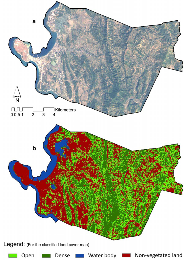
This study has used medium-resolution RS satellite images and GIS techniques to examine changes in vegetation cover from 1989 to 2009 in the barangays of the city of San Fernando, La Union, the Philippines, as input in planning vegetation rehabilitation. The vegetation cover change detection and analysis revealed that there were gains and losses of vegetation cover in most of the barangays in San Fernando during the said period. However, despite a decrease in vegetation, especially in ‘dense’ vegetation cover, in some of the urban barangays, there was an overall increase during the 20-year period. This is largely due to the reforestation efforts of both the barangays and the city government of San Fernando. Unfortunately, as there is no report on the survival rates of the planted trees, it is difficult to ascertain the degree of success of the reforestation activities, especially in the rural barangays. Nevertheless, the initiatives taken seem to have paid off, as shown by the results of this study.
The current initiatives of the city government are aimed at ensuring substantial protection and conservation of its entire natural environment amidst the critical challenges of sustainable urbanisation. The management of forested and degraded areas has been one of the current environmental rehabilitation, protection and conservation programs of the city. Other programs include management of the coastal areas and solid wastes, the clean air program, and the water and sanitation program, amongst others [37]. San Fernando has also enacted ordinances in relation to environmental protection and conservation. The most comprehensive was the City Ordinance No. 2006–013, otherwise known as the Environment Code of the City of San Fernando. In fact, San Fernando has been a recipient of numerous awards related to its initiatives in environmental rehabilitation, protection and conservation. For taking steps to conserve the environment, especially its vegetation cover, the city was the 2nd Runner-up in the Award for the Cleanest and Greenest City in the Philippines in 2003. In 2007, it won the Likas Yaman Award for Environmental Excellence by the Department of Environment and Natural Resources, Region 1 [37]. The numerous other awards received by the city in recent years, reflects the success of the city in delivering quality service to its people and in responding to the challenges of urbanisation. The success achieved by San Fernando city may persuade other municipalities in the province, and other cities in the region, to consider undertaking similar projects that would have a positive impact on the environment.
However, the loss of vegetation cover, especially in urban areas, is one problem that the city still has to resolve. In a city like San Fernando, urban forestry and urban greening, which focus on the management of urban green spaces comprising tree stands and individual trees [58], may be adopted and implemented. The barangays that showed losses of ‘dense’ and ‘open’ vegetation cover due to conversion to ‘non-vegetated land’, as well as those that showed substantial net losses in vegetation cover need to be prioritised in the rehabilitation planning. With the passing of Executive Order No. 26 on 24 February 2011 by the national government, which was created to implement the National Greening Program—to plant 1.5 billion trees in 1.5 million ha by 2016 [59], it is also expected that more reforestation projects will be undertaken by the barangays and the city government of San Fernando. In principle, the barangay officials, headed by their respective Captains, identify the areas for vegetation rehabilitation. This information is input during the strategic planning by the city government in which the barangay officials are involved. With support from the provincial government, the Department of Environment and Natural Resources (DENR), and other government agencies, including non-government organisations, the city government, who subsidises the rehabilitation programs by providing tree-planting materials, supervision and technical expertise, prioritises those barangays that require immediate attention. In this instance, the RS/GIS-generated information would be useful to the government at both city and barangay levels.
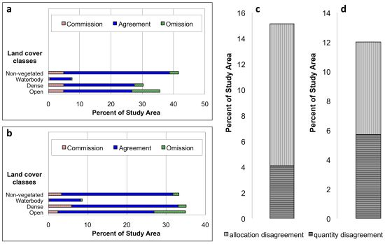
The RS/GIS methodologies used in this case study have demonstrated their usefulness and applicability in the monitoring of barangay-based vegetation cover changes. The classification method using a relatively small number and more general land cover classes, which did not require the pixels to be trained, but allowed the pixels to be classified based on their original spectral values, performed relatively well. The two parameters used in the accuracy assessment of the land cover maps; namely quantity disagreement and allocation disagreement, provide additional important information that the proportions correct and the standard Kappa index of agreement cannot offer. For example, the relative proportions of the two parameters can be used as a basis in determining whether the achieved accuracy levels of the land cover maps strongly support, and/or are appropriate for quantity-based or spatially-based analysis. However, a more specific baseline, particularly on what proportion of quantity or allocation disagreement is acceptable for a particular type of analysis, is yet to be established.
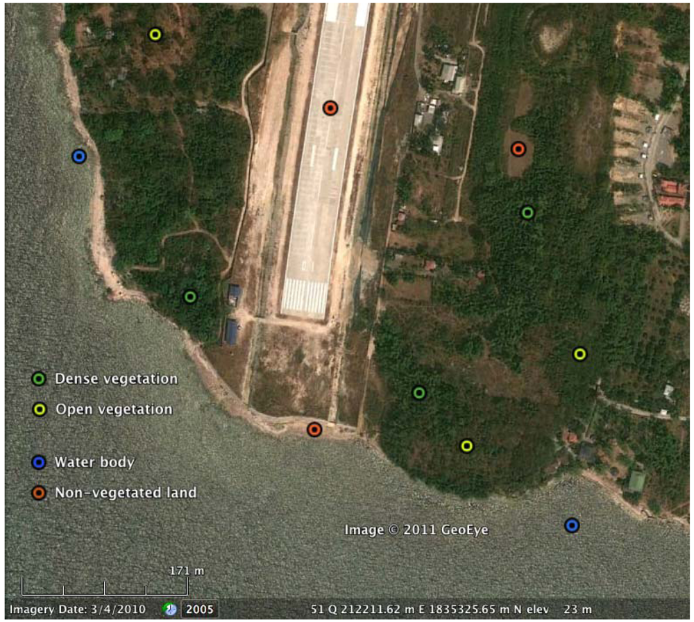
Extending the analysis down to the lowest level of the administrative hierarchy shows an indirect and a modest recognition of the significant role of these units in the rehabilitation, protection and conservation of the environment. The barangays hold very important, first-hand information on how changes in the vegetation cover occur and thus, these barangays, if explicitly involved, may give significant input in the rehabilitation, protection and conservation planning activities. In general, this study has contributed to the understanding of the vegetation cover changes in San Fernando, and will form the basis of the spatial decision-making processes for the environmental rehabilitation, protection and conservation efforts of the city and its barangays. We recommend, however, that the results of this study should be interpreted and used with careful consideration of the accuracy/inaccuracy levels of the classified land cover maps. This is because a part of the land cover change presented could be due to the time difference of the two RS satellite images used. In addition, the different spatial characteristics (e.g., scale/resolution) of the reference data used could also be one source of error affecting the accuracy of the results. Furthermore, it should not be forgotten that the changes in vegetation cover were analysed using land cover maps classified from images captured during the dry season. Land/vegetation cover mapping and change detection using images captured during the wet season should be one of the important concerns for future studies.
Nonetheless, this study has shown the suitability of the application of medium-resolution satellite images in obtaining information about the past and present vegetation cover in the study area. The approach implemented in this study can be used for similar studies in areas where up-to-date information on vegetation cover and cover conversions is as yet unavailable. Such information is extremely valuable for decision making at the lower administrative level, such as the barangay level. However, because in the Philippines most RS/GIS technologies are not yet accessible to the public, and the associated databases are yet to be developed for public use, the city government of San Fernando and its barangays, have to work hand-in-hand with the agencies that are already using these technologies, like the National Mapping and Resource Information Authority (NAMRIA), National Economic and Development Authority (NEDA), and Department of Environment and Natural Resources (DENR). Investment on RS/GIS software, database and technical staff development is needed.

Acknowledgements

The authors wish to thank the editors and the two anonymous reviewers whose constructive feedback helped to improve this paper. Likewise to the city government of San Fernando, particularly the Office of the Mayor, for approving the request to gather data for this study from the concerned units, and to the staff of the City Environment and Natural Resources Office for their support.

References and Notes

  1. de Sherbinin, A. Land-Use and Land-Cover Change—A CIESIN Thematic Guide; Columbia University: Palisades, NY, USA, 2002. Available online: http://sedac.ciesin.columbia.edu/tg/ guide_main.jsp (accessed on 29 October 2010).
  2. Lambin, E.F.; Baulies, X.; Bockstael, N.; Fischer, G.; Krug, T.; Leemans, R.; Moran, E.F.; Rindfuss, R.R.; Sato, Y.; Skole, D.; Turner, B.L., II; Vogel, C. Land-Use and Land-Cover Change (LUCC) Implementation Strategy. In IGBP Report 48 and IHDP Report 10; Nunes, C., Augé, J.I., Eds.; IGBP: Stockholm, Sweden, 1999; pp. 1–31. [Google Scholar]
  3. Lu, D.; Mausel, P.; Brondizio, E.; Moran, E. Change detection techniques. Int. J. Remote Sens. 2004, 25, 2365–2407. [Google Scholar] [CrossRef]
  4. Bakr, N.; Weindorf, D.C.; Bahnassy, M.H.; Marei, S.M.; El-Badawi, M.M. Monitoring land cover changes in a newly reclaimed area of Egypt using multi-temporal Landsat data. Appl. Geogr. 2010, 30, 592–605. [Google Scholar] [CrossRef]
  5. Asia-Pacific Network for Global Change Research (APN), Land Use and Land Cover Change in Southeast Asia: A Synthesis Report; 2001-13; APN: Kobe, Japan, 2001.
  6. Gunawan, I.; Skole, D.; Sanjaya, H.; Rahmadi, A.; Muchlis, M; Adi, G.A.; Gandharum, L.; Agus, A.B. Southeast Asia Regional Global Observation of Forest Cover Report No. 1; Directorate of Technology for Natural Resources Inventory, Agency for the Assessment and Application of Technology: Jakarta, Indonesia, 2000. [Google Scholar]
  7. Ong, P.S. The State of Philippine Biodiversity: Changing Mindscapes amidst the Crisis. In The 7th International Conference on Philippine Studies (ICOPHIL), Leiden, The Netherlands, 16–19 June 2004.
  8. Guarin, F.Y. Water quality management issues in Lingayen Gulf, Philippines and some proposed solutions. Marine Pollut. Bull. 1991, 23, 19–23. [Google Scholar] [CrossRef]
  9. Gaillard, J.C.; Liamzon, C.C.; Villanueva, J.D. ‘Natural’ disaster? A retrospect into the causes of the late-2004 typhoon disaster in Eastern Luzon, Philippines. Environ. Hazards 2007, 7, 257–270. [Google Scholar] [CrossRef]
  10. Pamintuan, M. Protect Philippine Forests; Philippine Daily Inquirer: Manila, Philippines, 2011. [Google Scholar]
  11. Saldivar-Sali, A.; Einstein, H.H. A landslide risk rating system for Baguio, Philippines. Eng. Ecol. 2007, 91, 85–99. [Google Scholar]
  12. United Nation-Food and Agriculture Organization (UN-FAO), Forests and Floods: Drowning in Fiction or Thriving on Facts? FAO and CIFOR: Bogor Barat, Indonesia, 2005.
  13. Hamilton, L.S.; Pearce, A.J. Biophysical Aspects in Watershed Managemen. In Watershed Resources Management: An Integrated Framework with Studies from Asia and the Pacific; Easter, K.W., Dixon, J.A., Hufschmidt, M.M., Eds.; Westview Press: Boulder CO, USA, 1986; pp. 33–52. [Google Scholar]
  14. Kummer, D. Deforestation in the Postwar Philippines; University of Chicago Press: Chicago, IL, USA, 1992. [Google Scholar]
  15. Revilla, J.A.V.; Javier, E.Q.; Vergara, N.T.; Gendrano, O.A. Quo Vadis, Philippine Forestry: toward Environmental Disaster or on to Sustainability (Forestry 2050); 2000; Unpublished report. [Google Scholar]
  16. Department of Environment and Natural Resources (DENR), Compendium of Basic Environment and Natural Resources (ENR) Statistics for Operations and Management, 2nd ed; DENR: Manila, Philippines, 2008.
  17. Estoque, R.C.; Murayama, Y. Spatio-temporal urban land use/cover change analysis in a hill station: The case of Baguio City, Philippines. Procedia-Social and Behavioural Sciences 2011, 21, 326–335. [Google Scholar]
  18. Araya, Y.H.; Cabral, P. Analysis and modelling of urban land cover change in Setúbal and Sesimbra, Portugal. Remote Sens. 2010, 2, 1549–1563. [Google Scholar] [CrossRef]
  19. Jaimes, N.B.P.; Sendra, J.B.; Delgado, M.G.; Plata, R.F. Exploring the driving forces behind deforestation in the state of Mexico (Mexico) using geographically weighted regression. Appl. Geogr. 2010, 30, 576–591. [Google Scholar] [CrossRef]
  20. Khoi, D.D.; Murayama, Y. Forecasting areas vulnerable to forest conversion in the Tam Dao National Park region, Vietnam. Remote Sens. 2010, 2, 1249–1272. [Google Scholar] [CrossRef]
  21. Poelmans, L.; Rompaey, A.V. Detecting and modeling spatial patterns of urban sprawl in highly fragmented areas: A case study in the Flanders–Brussels region. Landscape Urban Plan. 2009, 93, 10–19. [Google Scholar] [CrossRef]
  22. Dewan, A.M.; Yamaguchi, Y. Land use and land cover change in Greater Dhaka, Bangladesh: Using remote sensing to promote sustainable urbanization. Appl. Geogr. 2009, 29, 390–401. [Google Scholar] [CrossRef]
  23. Batisani, N.; Yarnal, B. Urban expansion in Centre County, Pennsylvania: Spatial dynamics and landscape transformations. Appl. Geogr. 2009, 29, 235–249. [Google Scholar] [CrossRef]
  24. Thapa, R.B.; Murayama, Y. Examining spatiotemporal urbanization patterns in Kathmandu Valley, Nepal: Remote sensing and spatial metrics approaches. Remote Sens. 2009, 1, 534–556. [Google Scholar] [CrossRef]
  25. Brink, A.B.; Eva, H.D. Monitoring 25 years of land cover change dynamics in Africa: A sample based remote sensing approach. Appl. Geogr. 2009, 29, 501–512. [Google Scholar] [CrossRef]
  26. Lee, Y.J.; Park, M.J.; Park, G.A.; Kim, S.J. A Modified CA-Markov Techniques for the Prediction of Future Land Use Change. In Proceedings of 2008 ASABE Annual International Meeting, Providence, RI, USA, 29 June–2 July 2008.
  27. Huang, Q.H.; Cai, Y.L. Simulation of land use change using GIS-based stochastic model: The case study of Shiqian County, Southwestern China. Stoch. Environ. Res. Risk Assess. 2007, 21, 419–426. [Google Scholar] [CrossRef]
  28. Shalaby, A.; Tateishi, R. Remote sensing and GIS for mapping and monitoring land cover and land use changes in the Northwestern coastal zone of Egypt. Appl. Geogr. 2007, 27, 28–41. [Google Scholar] [CrossRef]
  29. Kamusoko, C.; Aniya, M. Land use/cover change and landscape fragmentation analysis in the Bindura District, Zimbabwe. Land Degrad. Develop. 2007, 18, 221–233. [Google Scholar] [CrossRef]
  30. Xiao, J.; Shen, Y.; Ge, J.; Tateishi, R.; Tang, C.; Liang, Y.; Huang, Z. Evaluating urban expansion and land use change in Shijiazhuang, China, by using GIS and remote sensing. Landscape Urban Plan. 2006, 75, 69–80. [Google Scholar] [CrossRef]
  31. Mundia, C.N.; Aniya, M. Analysis of urban land use/cover change and urban expansion of Nairobi city using remote sensing and GIS. Int. J. Remote Sens. 2005, 26, 2831–2849. [Google Scholar] [CrossRef]
  32. Weng, Q. Land use change analysis in the Zhujiang Delta of China using satellite remote sensing, GIS and stochastic modeling. J. Environ. Manage. 2002, 64, 273–284. [Google Scholar] [CrossRef]
  33. Broich, M.; Hansen, M.C.; Potapov, P.; Adusei, B.; Lindquist, E.; Stehman, S. Time-series analysis of multi-resolution optical imagery for quantifying forest cover loss in Sumatra and Kalimantan, Indonesia. Int. J. Appl. Earth Obs. Geoinf. 2011, 13, 277–291. [Google Scholar]
  34. Lasco, R.D.; Pulhin, F.B. Forest land use change in the Philippines and climate change mitigation. Mitigation and Adaptation Strategies for Global Change 2000, 5, 81–97. [Google Scholar] [CrossRef]
  35. Republic Act (RA) 7160, Local Government Code of 1991; Congress of the Philippines: Manila, Philippines, 1991.
  36. National Mapping and Resource Information Authority (NAMRIA), Topographic Map of San Fernando, La Union; NAMRIA, DENR: Manila, Philippines, 1977.
  37. The City Government of San Fernando. The Official Website of the City of San Fernando, La Union, Philippines. 2011. Available online: www.sanfernandocity.gov.ph (accessed on 29 October 2010).
  38. National Statistics Office (NSO), Census of Population; NSO: Manila, Philippines, 2007.
  39. National Statistics Office (NSO), Census of Population; NSO: Manila, Philippines, 2000.
  40. National Statistics Office (NSO), Census of Population; NSO: Manila, Philippines, 1995.
  41. Estoque, R.C.; Murayama, Y. Suitability analysis for beekeeping sites in La Union, Philippines, using GIS and multi-criteria evaluation techniques. Res. J. Appl. Sci. 2010, 5, 242–253. [Google Scholar] [CrossRef]
  42. Tamesis, F. Philippine forests and forestry. Unasylva 1948, 2, 324–325. [Google Scholar]
  43. Tommervik, H.; Hogda, K.A.; Solheim, I. Monitoring vegetation changes in Pasvik (Norway) and Pechenga in Kola Peninsula (Russia) using multitemporal Landsat MSS/TM data. Remote Sens. Environ. 2003, 85, 370–388. [Google Scholar] [CrossRef]
  44. Anderson, J.R.; Hardy, E.E.; Roach, J.T.; Witmer, R.E. A Land Use and Land Cover Classification System for Use with Remote Sensor Data; US Geological Survey Professional Paper 964; US GPO: Washington, DC, USA, 1976. [Google Scholar]
  45. Yang, X.; Lo, C.P. Using a time series of satellite imagery to detect land use and cover changes in the Atlanta, Georgia. Int. J. Remote Sens. 2002, 23, 1775–1798. [Google Scholar] [CrossRef]
  46. Vanderee, D.; Ehrlich, D. Sensitivity of ISODATA to changes in sampling procedures and processing parameters when applied to AVHRR time-series NDVI data. Int. J. Remote Sens. 1995, 31, 136–145. [Google Scholar]
  47. Lins, K.S.; Kleckner, R.L. Land cover mapping: An overview and history of the concepts. In Gap Analysis: A Landscape Approach to Biodiversity Planning; Scott, J.M., Tear, T.H., Davis, F., Eds.; ASPRS: Bethesda, MD, USA, 1996; pp. 57–65. [Google Scholar]
  48. Congalton, R.G. A review of assessing the accuracy of classifications of remotely sensed data. Remote Sens. Environ. 1991, 37, 35–46. [Google Scholar] [CrossRef]
  49. Congalton, R.G.; Green, K. Assessing the accuracy of remotely sensed data: Principles and practices, 2nd ed; CRC Press: Boca Raton, FL, USA, 2009. [Google Scholar]
  50. Pontius, R.G.; Millones, M. Death to Kappa: Birth of quantity disagreement and allocation disagreement for accuracy assessment. Int. J. Remote Sens. 2011, 32, 4407–4429. [Google Scholar] [CrossRef]
  51. Foody, G.M. Harshness in image classification accuracy assessment. Int. J. Remote Sens. 2008, 29, 3137–3158. [Google Scholar] [CrossRef]
  52. Allouche, O.; Tsoar, A.; Kadmon, R. Assessing the accuracy of species distribution models: prevalence, kappa and true skill statistic (TSS). J. Appl. Ecol. 2006, 43, 1223–1232. [Google Scholar] [CrossRef]
  53. Foody, G.M. Thematic map comparison: evaluating the statistical significance of differences in classification accuracy. Photogramm. Eng. Remote Sensing 2004, 70, 627–633. [Google Scholar]
  54. Di Eugenio, B.; Glass, M. The kappa statistic: A second look. Computat. Linguist. 2004, 30, 95–101. [Google Scholar] [CrossRef]
  55. Eastman, J.R. IDRISI Taiga Tutorial; Clark University: Worcester, MA, USA, 2009. [Google Scholar]
  56. Yu, H.; Joshi, P.K.; Das, K.K.; Chauniyal, D.D.; Melick, D.R.; Yang, X.; Xu, J. Land use/cover change and environmental vulnerability analysis in Birahi Ganga sub-watershed of the Garhwal Himalaya, India. Tropical Ecol. 2007, 48, 241–250. [Google Scholar]
  57. Mehaffey, D. Deforestation and Forest Management in the Philippine Provinces of Benguet and La Union. M.Sc. Dissertation, University of Wales Bangor, Gwynedd, UK, 2004. [Google Scholar]
  58. Bentsen, P.; Lindholst, A.C.; Konijnendijk, C.C. Reviewing eight years of urban forestry & urban greening: Taking stock, looking ahead. Urban For. Urban Green. 2010, 9, 273–280. [Google Scholar] [CrossRef]
  59. Executive Order (EO) No. 26, An Order for the Implementation of the National Greening Program (NGP) of the Philippines; Office of the President of the Republic of the Philippines: Manila, Philippines, 2011.
  60. ERDAS, ERDAS Field Guide; ERDAS Inc: Norcross, GA, USA, 2009.
  61. Kamusoko, C.; Oono, K.; Nakazawa, A.; Wada, Y.; Nakada, R.; Hosokawa, T.; Tomimura, S.; Furuya, T.; Iwata, A.; Moriike, H.; et al. Spatial simulation modeling of future forest cover change scenarios in Luangprabang Province, Lao PDR. Forests 2011, 2, 707–729. [Google Scholar] [CrossRef]

