A New Algorithm for Identifying Possible Epidemic Sources with Application to the German Escherichia coli Outbreak

Abstract

In this paper we describe a recently developed algorithm called Topological Weighted Centroid (TWC). TWC takes locations of an event of interest and analyzes the possible associated dynamics using the ideas of free energy and entropy. This novel mathematical tool has been applied to a real world example, the epidemic outbreak caused by Escherichia coli that occurred in Germany in 2011, to point out the real source of the outbreak. Other four examples of application to other epidemic spreads are described: Chikungunya fever of 2007 in Italy; Foot and mouth disease of 1967 in England; Cholera of 1854 in London; and the Russian influenza of 1889–1890 in Sweden. Comparisons have been made with other already published algorithms: Rossmo Algorithm, NES, LVM, Mexican Prob. The TWC results are significantly superior in comparison with other algorithms according to four independent indexes: distance from the peak, sensitivity, specificity and searching area. They are consistent with the idea that the spread of infectious disease is not random but follows a progression based on inherent, but as yet undiscovered, mathematical laws. The TWC method could provide an additional powerful tool for the investigation of the early stages of an epidemic and novel simulation methods for understanding the process through which a disease is spread.

1. Introduction

In a previous paper we introduced for the first time a new mathematical approach (H-PST Algorithm) to identify the possible location of an epidemic outbreak source [1] showing that a distribution of events generated by the same process in a two dimensional space has a wealth of hidden information. We compared this new artificial intelligence method with other well-known algorithms to identify the source of three examples of infectious disease outbreaks derived from literature. The H-PST algorithm is a system able to project a distance matrix of points (events) into a bi-dimensional space with the generation of a new point that has been named the hidden unit. This new hidden unit deforms the original Euclidean space and transforms it into a new space (cognitive space). The cost function of this transformation is the minimization of the differences between the original distance matrix among the assigned points and the distance matrix of the same points projected into the bi-dimensional map. The position of the hidden unit proved to effectively target the outbreak source in many epidemics much better than the other classic algorithms specifically targeted for this task. This study shows clearly that one possible hidden piece of information that can be revealed is the location from which the event originated. To adequately understand the history of this method the reader is directed to [1,2].

From the beginning, however, we were aware of some limitations of this technique. In fact, the H-PST algorithm is very efficient when the point distances do not follow either the Euclidean or Manhattan metrics (time distances, curvilinear distances, etc.), but less efficient when the point distances fit a two-dimensional map. In addition, H-PST defines the search area as a single point and not as a probability area. This has prompted us to develop a more accurate algorithm with a multivalent performance. The algorithm presented here is called the Topological Weighted Centroid (TWC) and was designed in 2008 [3,4] at Semeion Research Center. It minimizes the global entropy among the positions of the points where the events occurred using no additional information but able to point out the position of a hidden “point zero” (the source of the process), taking historical information only from the already manifested precise positions of the other events together with other interesting mathematical entities. This discovery suggests that every static distribution of points in a two dimensional space could implicate new information about their dynamics.

This paper is organized into sections:

In Section 2 we present a series of mathematical entities that the TWC algorithm generated:

• A new point, the TWC Alfa, and a new scalar field, the TWC Alfa Map: these two entities constitute an estimation of the outbreak of the assigned epidemic;
• A scalar field, the TWC Beta, whose goal is to show the possible diffusion map of the epidemic;
• Another scalar field, the TWC Gamma, and other mathematical entities show an estimation of the future diffusion of the epidemic.

In Section 3 we present four different and well known cases of epidemics whose outbreaks are well known:

• Case 1: The Chikungunya fever epidemic of 2007;
• Case 2: The Foot and mouth disease epidemic of 1967 in Great Britain;
• Case 3: The Golden Square cholera epidemic of 1854 in London;
• Case 4: The Russian influenza in Sweden in 1889–1890;

In Section 4 we will present and compare the effectiveness of TWC-α algorithm with other algorithms known in the geographic profiling field:

• The Rossmo Algorithm [5];
• Negative Exponential Summation Algorithm (NES) [1];
• Likelihood Variance Maximization Algorithm (LVM) [1];
• Mexican Probability Algorithm (Mex Prob) [4].

We have decided not to consider certain trivial algorithms such as the spatial central tendency because they have already been shown to be too naive and not competitive (Le Comber [6], Stevenson [7]).

We have also decided not to consider certain other approaches including temporal information and frequencies in the epidemic dynamics. We have already proposed new algorithms to cope with these richer datasets (see Buscema [8]). In this paper we want to show only the possibility of obtaining the maximum of information from the crude spatial distribution of a set of events (points with latitude and longitude) in bi-dimensional space.

In Section 5 we will present the results of the comparison and propose a methodology, composed of four indicators, to evaluate the performances of any algorithm in geographic profiling:

• The Distance of the peak of the map from the target (outbreak);
• The Sensitivity of the target location on the map;
• The Specificity of the target location on the map;
• The Percent of the searching area proposed by any algorithm.

In Section 6 we provide a first validation of the predictive capability of TWC methodology using 12 months of data collecting concerning a food epidemic in OAHU (Hawaii) in 2010.

Finally, in Section 7 we demonstrate the efficacy of TWC in the epidemic outbreak that occurred in Germany in 2010, the hemolytic uremic syndrome (HUS) epidemic in which over 40 deaths occurred in a two month period. Section 7 is also addresses the conclusions.

2. The Topological Weighted Centroid Algorithm

2.1. Some Mathematical Details about TWC-α Method

The points at which an event of interest occurs are called the assigned points. The center of mass of the assigned points represents the point at which the maximum entropy occurs.

Let N = Number of assigned points and K = Number of all the points of the two-dimensional plane on a chosen/fixed grid. Then the coordinates of the center of mass are defined by the following equation:

(1)

where Px_r and Py_r are and y of the assigned point.

The center of mass has the following property:

(2)

(3)

where Cx_r and Cy_r are and of the point in the pane and is the sum of the square of the distance of point C_r from the assigned point P_i.

Now, if we re-write the Equation (1) giving a specific weight to each of the assigned points and also weight the distance between two points by the average (modified) distance that each point has from the others, we generate Equation (4):

(4)

where

(5)

(5a)

and where D = maximum distance among the assigned points, modified distance between two of the assigned points, d_i,j,d_i,k = Euclidean distance between two of assigned points, and .

The weight is defined by Equation (5). Equation (4) is the same as Equation (1) but is weighted by Equation (5).

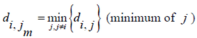
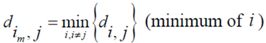
Equation (5a) changes the final attractor of TWC (α_n), as n→∞, into a non-trivial attractor. With Equation (5a) for each distance (d_i,j) we take into account the average of the other distances (d_i,k, with k ≠ i and k ≠ j). In fact, without Equation (5a), the convergence point of TWC(α_n), as n→∞, corresponds to the mean of the two points having the minimal Euclidean distance (see the proof in Appendix A), while by Equation (5a) the final attractor is the point in space whose average distance from the other points is minimal. This point need not be unique because the matrix of the distances generated by Equation (5a) is not symmetric (see Appendix B).

Now, we find the vector of optimal weights (Equation (5)), having the following properties:

(6)

(7)

(8)

(9)

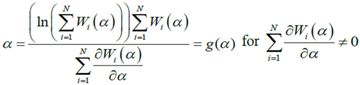
We have developed an algorithm to optimize Equation (6) as follows:

• Initialize α₍₀₎ = 0 at first cycle; all the components of the vector w(α_n) at this point will be equal to 1 and the TWC (α_n) will have the same coordinates of the center of mass.
• At the next cycle increase α with a small positive quantity:
• The Equations (7) and (8) will show an entropy reduction and an increasing of the free energy (see Appendix C), and then the TWC (α_n) will move in a specific direction of the plane (Equation (4)).
• When the free energy (Equation (7)) attains the global max, the process terminates at α^* = α_n.

The conditions for existence of a convergent point, that is, convergence to a (unique) point, is associated with the conditions for convergence to the (unique) point of Newton’s Method. Alternatively, one could analyze this algorithm from a Fixed Point Algorithm point of view (see Appendix D). The path described by the TWC (α_n) evolution is also very informative and can be retained for at least two reasons:

• All the TWC (α_n) points represent the best path with which to reach the maximum of the free energy of the weighted mean of the assigned points, starting from the center of mass. This path is usually nonlinear and a non-monotonic curve.
• The set of points belonging to the TWC (α_n) trajectory can be used to transform the plane into a scalar field, TWSF (α_n), where the proximity of each geometrical point to this trajectory can be measured.

The TWC (α^*) represents, therefore, the point at which the weighted mean of the assigned points represents the maximum free energy. In many applications this remarkable point can represent, or point out, the source of the process because this point is also the point where the entropy is minimal, so it is the point from which (if you were to put yourself there) other points generate maximum information; in other words this is the point of Negentropy. On the other hand, the center of mass is the point where the entropy is maximum, so it is also the point from which (if you were to put yourself there) the distribution of assigned points is least informative. We can also find α^* by using a Newton’s Method or the fixed point algorithm (see appendix D). Conditions associated with Newton’s Method or the fixed point algorithm indicates existence and uniqueness of the method that is convergence to a unique solution.

2.2. Details of TWC-β Method

Now we change Equation (5) to the following form:

(10)

Equation (10) presents a dynamic different to that of Equation (5). Specifically, when the parameter β is still small, the system entropy will decrease, but for larger values of β the distance of any point from itself (which is included in the Equation (10)) will prevail and the trajectory of the TWC points will come back to the center of mass, with a consequent increase in entropy. So, with Equation (10) we target a different direction: the trajectory leaves the center of mass and then returns to the point in question. This means we can try to define the optimal value of β for which the entropy of the weighted mean of the assigned points is minimal when we include it into the weights calculation and the pseudo-distance of each point from itself. This is the β^* for which point TWC (β^*) of the trajectory begins to turn back. This is because v_i(β^*) is the vector of weights defined by a specific value of β, where the entropy is the smallest (β^*) as computed by the following:

(11)

(12)

(13)

(14)

The x and y components of are given:

(15)

Also, the iterative algorithm in which the β parameter has increased is necessary according to Equation (14) because we do not a priori know which value of β satisfies the statement in Equation (11) and gives β = β^* (See Appendix A from Equation (A16) to Equation (A22)).

The β^* parameter will now be used to define the proximity of each geometrical point (all the grid points that define the space) to the assigned points:

N; {Number of assigned points}

M; {Number of points of the discretized space}

i,j {1,2,…,N}; {Assigned points indexes}

k {1,2,…,M}; {geometrical points index}

(16)

{Euclidean distance between any couple of assigned points}

(17)

{Maximum distance among the assigned point}

(18)

{Euclidean distance between any geometrical point and any assigned point}

(19)

Note: p_k has been changed to TWSF (β^*).

{Proximity of each geometrical point to all assigned points, with β^* as parameter minimizing the entropy}

Equation (19) gives the TWC-β scalar field, TWSF (β^*), which is generated from the β^* parameter.

2.3. Some Mathematical Details of TWC-γ Method

The TWC (γ_i) analyzes the weighted distances of each of the assigned points from the other. In fact, the TWC (γ_i) is the set of points connecting the center of mass to each one of the assigned points. Consequently, each one of the assigned points will be described by a vector, z, of weights.

Components of each vector define a set of TWC (γ_i) points for each of the assigned points. Therefore, each component of this set of points represents the weighted average of all the points with respect to an increasing value of the γ parameter, in relation to any one of the assigned points. The starting point of each TWC (γ_i) is located at the center of mass. Now the last TWC (γ_i) terminates at the point where for each of the assigned points the entropy of the weighted average is minimized according to Equation (29).

The following equations illustrate the algorithm that calculates the TWC (γ_i):

(20)

{Euclidean distance between the i-th and the j-th entity}

(21)

{Maximum distance among the assigned point}

(22)

{γ-dependent proximity between the i-th and the j-th entities}

(23)

{Coordinates of the i-th Weighted Centroid at the step t}

(24)

(25)

(26)

{Entropy of the i-th point at the step t}

(27)

{Normalization of the weights}

(28)

{Condition of Termination}

(29)

Thus TWC (γ_i) defines a set of trajectories whose dynamics is the output of the many-to-many interactions among the distances of all the assigned points. The TWC-γ map is the scalar field, TWSF (β^*(γi)), measuring the global proximity of each geometrical point of the two-dimensional space to all these TWC (γ_i) trajectories.

The following equations detail the algorithm to generate the TWC-γ scalar field, TWSF (β^*(γ_i)):

Legend:

N= Number of points composing all the trajectories points, TWC (γ_i), in the discrete space;

M=Number of geometrical points of the discrete space;

i,j {1,2,…,N}; {Indexes for the trajectories points}

k {1,2,…,M}; {Index for the geometrical points}.

{Euclidean distance between each geometrical points and each trajectories points}

(30)

{Proximity of a point to the trajectory points, with β^* parameter}

(31)

Equation (31) gives the TWC-γ scalar field, TWSF (β^*(γi)) which depends on the β^* parameter.

2.4. A Short Synthesis of TWC Method

TWC (α^*) is a new point of the space from which the other assigned points (input data points of interest) have minimum entropy with maximum free energy. This point has been shown to mark the source of the dynamic process underlying the occurrence of points of interest. This prediction tool has a number of benchmark algorithms described in Section 4. The set of points belonging to the TWC (α_k), k = 0,1,… trajectory transforms the plane into a scalar field where the proximity of each geometrical point (points on the grid of the map) to this trajectory can be measured. Parameter β^* is the critical value of β at which the entropy of the weighted mean of the assigned points is minimal and it is used to define the TWC-β scalar field, TWSF (β^*). The diffusion probability could be calculated by measuring the intensity of the scalar field. The diffusion probability determines the probability that a new event could occur at a geometrical point of the map. A scalar field in physics is basically used to associate a scalar value (like temperature or electric potential energy) to every point in the space. The gradient (or minus the gradient) of a scalar field is a vector field, for example, the negative gradient of electric potential is the electric field. Therefore the TWSF (β^*) represents a property of the space which is similar to electric potential. We will interpret these points, trajectories, and scalar fields as possible sources of the disease or indicators as to where the disease will next spread.

The set of points, TWC (γ_i), provides information about the weighted distances of each of the assigned points from the others. TWC (γ_i) is the set of points connecting the center of mass to each one of the assigned points. TWC (γ_i) can be used to build up a matrix of nonlinear trajectories connecting the points of interest, which may be interpreted as the dynamic movement of the disease outbreak. The TWC (β^*(γ_i)) points are transformed into a map that is the scalar field TWSF (β^*(γ_i)) measuring the global proximity of each geometrical point of the two-dimensional space to all of the TWC (γ_i) trajectories by using the β^* parameter. The point with minimum entropy and maximum free energy may be interpreted in context of many applications as a remarkable point that represents, or can point out, the source of a spreading phenomenon like an epidemic outbreak. TWC-β and TWC-γ sets of points do not yet have any benchmarking algorithm.

3. Four Epidemics Already Known

3.1. The Chikungunya Fever Epidemic of 2007

Chikungunya fever is a toga viral illness that is spread by the bite of infected mosquitoes of the Aedes Aegypti mosquitoes. Mosquitoes breed in stagnant or standing surface waters, puddles or oil drums and are infected by feeding on a sick individual. Chikungunya fever is characterized by severe, sometimes persistent, joint pain (arthritis) as well as fever and rash. The disease is debilitating but rarely life-threatening. The virus was first isolated between 1952–1953 from both man and mosquitoes during an epidemic of fever that was considered clinically indistinguishable from dengue, in Tanzania.

Up to 2007, no autochthonous cases had taken place outside these areas, but between July and August 2007, 205 cases of Chickungunya fever took place in the environs of the two northern villages of Castiglione di Cervia and Castiglione di Ravenna in Northern Italy. The spatial topography of the epidemic had a decreasing concentric gradient, with fewer cases taking place furthest from the epicenter. The probable index case was identified as a traveler from an area of India in which an epidemic of Chickungunya fever was underway and the highest concentration of cases was identified as the village of Castiglione di Cervia [9]. We have used the coordinates of the points corresponding to the outbreak status in the late phase of development.

3.2. The Foot and Mouth Disease Epidemic of 1967

The animal epidemic of Foot and Mouth disease (FMD) of 1968–1969 caused the death of 2,000 animals and the compulsory slaughter of half a million more and wrought economic chaos to the cattle and meat producing industries. The origin of the epidemic was traced to infected pig swill at Bryn Farm, near Oswestry in the English county of Shropshire [10]. Foot and mouth was not a new disease in the UK in 1967–1968. Throughout the 1950s and 1960s, it was not unusual to have outbreaks (sometimes two or three in a year) of FMD. From 1954 to 1967, excluding the 1967–1968 outbreak, there were 1,002 outbreaks with an average of 75 cases every year, and there were only two years, 1963 and 1964, when there was no disease, the longest period without the disease since 1908. In the 1967–1968 outbreak when the first case was diagnosed at Bryn Farm on 25 October, a Wednesday, the normal Oswestry market was taking place and two cows from that farm had gone to the market that morning. On the basis of disease recognition the State Veterinary Service decided immediately to close down the market. These two cows were examined the next day, 26 October and found free of the disease, but despite this they were included in the slaughter. Some animals had left and gone as far as Banffshire in Scotland and Devon in the south-west before the measures had been enacted. All these animals were traced and found healthy, so the decision was taken not to introduce compulsory slaughter of all the animals in the market. On Monday, 30 October, the situation changed dramatically when there were nine fresh cases confirmed, six close to the original outbreak. The other three were considerable distances away (12, 35 and 100 m, the furthest being in Lancashire). From 30 October on there was a dramatic escalation of cases which in the end involved 2,000 animals.

We have used the coordinates of the points corresponding to the 20 farms infested by the outbreak in the first week. The coordinates were derived from the map described of the published report [10].

3.3. The Golden Square Cholera Epidemic of 1854

John Snow (1813–1858), was a London physician who famously investigated the 1854 cholera epidemic around the Berwick Street area of Soho as part of a wider study to test his hypothesis that cholera was waterborne rather than, as most then believed, airborne. Snow further believed the vector of transmission was either personal contact with an infected person or the drinking of contaminated water in which some “morbid poison” travelled. He undertook two separate studies. One considered the correlation between water sources and the incidence of cholera in South London and the other examined a localized outbreak in London’s Soho District. The results of both studies were published in a second and greatly expanded edition of “On the Mode of Transmission of Cholera” in which Snow published for the first time the large-scale cholera outbreak map which in the twentieth century would become an icon for medical cartography [11].

This famous point source epidemic (part of an ongoing propagated source epidemic) was investigated in detail by Snow who talked to local residents and conducted door-to-door investigation, thus collecting the data to create the spot map to illustrate how cases of cholera were centered around the pump. He used bars to represent deaths that occurred at the specified households, and by weighting the density of these bars and relating them to the distance of neighborhood pumps he was able to confirm the Broad Street pump as the origin of the spread of the cholera outbreak. Snow’s use of his famous map was confirmatory rather than proof, as he had elaborated the focused underlying theory to explain the spread of water born cholera [12].

A full visual confirmation of the communication between the cesspool near number 40 and the nearby pump well was given in April 1855, four months after the publication of Snow’s classic on the Mode of Communication of Cholera, following a complete excavation of the cesspool by the parish council. It seems likely that the index case had been living with her parents at number 40 and her mother (Sarah Lewis) washed the sick’ baby’s diapers in the cesspool, allowing the vibrios to enter the water supply through communication between the cesspool and the pump well. Despite Snow’s desperate efforts, in the time between the 19 August and the 31 of (the beginning of the Golden Square epidemic), there were 73 cases of cholera and 12 deaths.

The intelligent discovery of the outbreak of the cholera epidemic has already been treated with modern mathematics and statistics [1,6].

The digital map is composed of 578 locations (buildings) and three repetitions that we have decided not to delete from the dataset. The data set reflects the final state of evolution of cholera epidemics.

3.4. The Russian Influenza in Sweden in 1889–1890

In 1890, immediately after the outbreak of Russian influenza, all Swedish doctors were asked to provide information about the start and the peak of the epidemic and the total number of cases in their region, and to fill in a questionnaire on the number, sex and age of infected persons in the households they visited.

General answers on the epidemic were received from 398 physicians and data on individual patients were available for more than 32,600 persons. From the answers a table was compiled and a map was drawn in 1890 indicating when the influenza first appeared at the various locations. To support the contagiousness theory an analysis of the railway network was done in relation to the onset of the outbreak. In the first week in December 1889, 12 of the 13 affected places outside Stockholm had railway stations. Linroth demonstrated that by 20 December, 82% of reporting places with a railway station and 47% without one had been affected [13].

The dissemination was very fast and the local epidemics developed at a pace that in some cases were described as explosive. Due to the general susceptibility, the short incubation time and the difficulty to detect the very first cases, more proof was needed to scientifically verify that the influenza was indeed contagious.

Linroth was, however, of the opinion that the many individual testimonies describing how the infection was transferred directly from infected persons justified the hypothesis: Influenza is a contagious disease.

In a recent GIS study [13], Linroth’s original tables were converted into Excel format and dot maps.

We have worked on the dots of week three using the coordinates of the points corresponding to the 44 locations interested by the outbreak in the third week, an early phase of evolution in temporal terms (number of cases per locations) but not in topological terms (number of locations with at least one case).

4. The Algorithms Used for Comparison with TWC-α

This class of algorithms focuses only upon the metric of the space, D^N and the shape of the decay distance function, F(D^N) and the sum as a composition function, S, without specific assumptions about other factors. Following this approach, the anchor point, Y^*, is located in a region with a high “Hit Score” [14]:

These approaches tend to define the probability of each point of the grid—within the convex hull of the locations of the observations—to be the outbreak. Consequently, the probability distribution strategy defines a search area whose points have a high probability to be the outbreak point [1,14].

4.1. The Rossmo Algorithm

The Rossmo Algorithm [5,6] uses the block (Manhattan) distance. It employs four free parameters, each of which has to be calibrated empirically according to the situation. This algorithm is specific to finding the anchor point in serial crimes. We adapted its four parameters and its metric to apply it in the field of the tracking of epidemics. The Rossmo equations are the following:

where: d = the distances among points, in any metric; B = the diameter of the protection zone, when it is the case; g and h = exponents governing the competition between the decay distance among points and the protection zone.

The first term of the equation takes its inspiration from Newtonian gravity. The whole equation represents a formulation of the Brantingham and Brantingham [15,16] search area model, in which the offender’s search behavior is seen as following a distance decay function with decreased activity near the offender’s home base. Rossmo has produced examples showing how the model can be applied to serial offenders [17]. For both the “within buffer zone” (near to home base, controlled by the parameter “B”) and “outside buffer zone” (far from home base) functions, the parameter “k” and the exponents “h” and “g” are empirically determined.

4.2. The Negative Exponential Summation Algorithm (NES)

The NES Algorithm [1] uses the buffer concept of the Rossmo model and the negative exponential of Canter [18,19,20,21,22], combining them in the following equations:

where: φ = The connection strength among the points; d = The distances among points, in any metric; B = The diameter of the protection zone, when it is the case; g and h = Exponents governing the competition between the decay distance among points and the protection zone.

When “h” and “g” are fine-tuned appropriately (h = 0.05 and g = 0.01), the NES Algorithm has proved to be very sensitive to the distribution of the observed sites [23,24].

4.3. The Likelihood Variance Maximization Algorithm (LVM)

The LVM Algorithm [1] is inspired to the maximum likelihood technique that O’Leary presents and rejects as a poor model in favor of a Bayesian approach [25]. But the strong point of this simple technique is the cost function: we try to maximize the variance of the likelihood among all the candidate operation points, by means of an iterative process:

σ and σ^* = the width (and the optimal width) of the bell of the decay function and σ^* = the width (and the optimal width) of the bell of the decay function.

The LVM Algorithm presents two main advantages: it does not need the setup of external parameters and it is based on Bayesian theory.

4.4. The Mexican Probability Algorithm (Mex Prob)

The MexProb algorithm [4] was created to manage within only one equation all the parameters usually employed in location theory algorithms:

φ = The connection strength among the points;

d = The distances among points, in any metric;

B = The diameter of the protection zone, when it is the case;

σ and σ^* = The width ( and the optimal width) of the bell of the decay function.

The MexProb algorithm, moreover, calibrates all these parameters by itself, by maximizing the variance of its scalar field, iteratively:

5. Results

5.1. The Results of the Comparison of the Four Algorithms with TWC

The TWC (α^*) and especially the TWFS (α_n) have been considered in this comparison, because they are very useful to estimate the outbreak of a points distribution.

As we mentioned the other algorithms that are considered in this benchmark are:

• Rossmo Algorithm [5,6]
• NES Algorithm [1]
• LVM Algorithm [1]
• Mex Prob Algorithm [4]

This experimentation was performed using the same software package [26].

Further, we have considered four different indices to compare the four algorithms with TWC:

• The distance from the peak of each algorithm to the real outbreak has been calculated as follows: it is basically relative distance and it is calculated relative to the main diagonal of the window grid generated by the software in percentage form. For each data distribution (dataset) our software draws a grid map of 600 × 600 pixels, where all the points all embedded in a sub window of 500 × 500 pixels.
• The sensitivity is defined as the value of the point of the scalar field of each algorithm (each pixel value of the scalar field generated by each algorithm is scaled between 0 and 1) in the place where the real outbreak is located. The specificity is defined as the percent value of the number of points of the whole window whose value is the smallest values of the sensitivity of each algorithm.
• The search area in which the real outbreak can be found in the scalar field of each algorithm is defined as following: we have divided the scalar field generated by each algorithm in 20 bins of equal length and then we calculate the extension of the area into which the real outbreak is included. Finally we express the value of this bin area in relation to the area of the global window.
• Table 1, Table 2, Table 3, Table 4 show the analytic results of the comparison while Table 5 shows the average rank that each algorithm performed in each test. Appendix E shows the maps projected by each algorithm for each epidemic.

Table 1. Foot and Mouth Disease results.

Foot and Mouth Disease
Algorithm	Distance from Outbreak	Sensitivity	Specificity	Search Area	Rank
TWC Alfa	0.7400%	94.6000%	99.9825%	0.0175%	1
Rossmo	6.1400%	90.6200%	99.7500%	0.2950%	2
NES	6.1400%	75.5700%	99.8650%	0.3700%	3
LVM	6.1400%	87.7400%	99.7600%	0.3775%	4
Mex Prob	6.0000%	83.3000%	99.7800%	0.5775%	5

Table 1. Foot and Mouth Disease results.

Foot and Mouth Disease
Algorithm	Distance from Outbreak	Sensitivity	Specificity	Search Area	Rank
TWC Alfa	0.7400%	94.6000%	99.9825%	0.0175%	1
Rossmo	6.1400%	90.6200%	99.7500%	0.2950%	2
NES	6.1400%	75.5700%	99.8650%	0.3700%	3
LVM	6.1400%	87.7400%	99.7600%	0.3775%	4
Mex Prob	6.0000%	83.3000%	99.7800%	0.5775%	5

Table 2. Chikungunya fever results.

Chikungunya Fever
Algorithm	Distance from Outbreak	Sensitivity	Specificity	Search Area	Rank
TWC Alfa	0.0000%	100.0000%	99.9650%	0.0000%	1
Rossmo	0.7300%	97.6600%	99.9800%	0.0200%	2
NES	1.0300%	96.2100%	99.9725%	0.0275%	3
LVM	0.7300%	98.7900%	99.8875%	0.1125%	4
Mex Prob	2.9100%	97.0600%	99.7500%	0.2500%	5

Table 2. Chikungunya fever results.

Chikungunya Fever
Algorithm	Distance from Outbreak	Sensitivity	Specificity	Search Area	Rank
TWC Alfa	0.0000%	100.0000%	99.9650%	0.0000%	1
Rossmo	0.7300%	97.6600%	99.9800%	0.0200%	2
NES	1.0300%	96.2100%	99.9725%	0.0275%	3
LVM	0.7300%	98.7900%	99.8875%	0.1125%	4
Mex Prob	2.9100%	97.0600%	99.7500%	0.2500%	5

Table 3. London cholera results.

London Cholera
Algorithm	Distance from Outbreak	Sensitivity	Specificity	Search Area	Rank
TWC Alfa	4.4900%	95.3100%	99.5375%	0.0025%	1
Mex Prob	5.1600%	93.7800%	99.3625%	0.4775%	2
LVM	5.1600%	96.0600%	99.2900%	0.7100%	3
NES	4.9600%	86.5100%	99.6575%	0.7350%	4
Rossmo	5.1600%	97.3900%	98.6800%	1.3200%	5

Table 3. London cholera results.

London Cholera
Algorithm	Distance from Outbreak	Sensitivity	Specificity	Search Area	Rank
TWC Alfa	4.4900%	95.3100%	99.5375%	0.0025%	1
Mex Prob	5.1600%	93.7800%	99.3625%	0.4775%	2
LVM	5.1600%	96.0600%	99.2900%	0.7100%	3
NES	4.9600%	86.5100%	99.6575%	0.7350%	4
Rossmo	5.1600%	97.3900%	98.6800%	1.3200%	5

Table 4. Russian influenza results.

Russian Influenza
Algorithm	Distance from Outbreak	Sensitivity	Specificity	Search Area	Rank
NES	3.9100%	85.1200%	99.8800%	0.2475%	1
TWC Alpha	3.1600%	67.8600%	99.8500%	0.4550%	2
Mex Prob	6.3200%	86.5800%	99.4050%	1.4900%	3
LVM	6.5500%	88.1100%	99.0975%	1.6525%	4
Rossmo	19.9300%	92.5400%	94.4700%	3.1150%	5

Table 4. Russian influenza results.

Russian Influenza
Algorithm	Distance from Outbreak	Sensitivity	Specificity	Search Area	Rank
NES	3.9100%	85.1200%	99.8800%	0.2475%	1
TWC Alpha	3.1600%	67.8600%	99.8500%	0.4550%	2
Mex Prob	6.3200%	86.5800%	99.4050%	1.4900%	3
LVM	6.5500%	88.1100%	99.0975%	1.6525%	4
Rossmo	19.9300%	92.5400%	94.4700%	3.1150%	5

Table 5. The average rank of each algorithm in the four tests.

Algorithm	Foot and Mouth	Chikungunya	London Cholera	Russian Influenza	Rank
TWC Alfa	1	1	1	2	1.25
NES	3	3	4	1	2.75
Rossmo	2	2	5	5	3.50
Mex prob	5	5	2	3	3.75
LVM	4	4	3	4	3.75

Table 5. The average rank of each algorithm in the four tests.

Algorithm	Foot and Mouth	Chikungunya	London Cholera	Russian Influenza	Rank
TWC Alfa	1	1	1	2	1.25
NES	3	3	4	1	2.75
Rossmo	2	2	5	5	3.50
Mex prob	5	5	2	3	3.75
LVM	4	4	3	4	3.75

These comparison results have been given according to the “searching area” as the key index to rank the algorithms’ performances, as recommended recently by some authors [19]. Using this criterion TWC performs better than all other four algorithms especially in 3 of the 4 tests. But also the other indices that we have introduced are relevant and they are not always correlated with the “searching area”.

The distance from the outbreak (r) is not a flawed metric [6]. It describes a circle of radius “r” whose area describes a meaningful “searching zone” and does not have an arbitrary link to the “binning strategy” chosen by the researchers. The searching area, in fact, may take different sizes in relation to the binning segmentation of the scalar field.

“Sensitivity” indicates how much each algorithm considers the position of the real outbreak a “hot location”. In other words, the searching area could be small but the real position of the real outbreak is not considered a location with a high probability value. A look at the “Foot and Mouth Disease” case, where all the algorithms tested, except TWC (α), shows an absence of very high values in the location where the outbreak is really located.

“Specificity” is a fundamental index to understand the percentile where the real outbreak is located. In “Russian Influenza” case, the Rossmo algorithm is shown to be quite generic in relation to the other methods: good sensitivity, but the lowest specificity.

At the end of this comparison we can add the following observations:

• All the algorithms have performed fairly well in each of the five tests (these four cases plus E-coli). That means that their foundation is robust and solid;
• The TWC (α) results have significantly shown this method to be more effective than the other algorithms (in most of the cases its searching area is one order of magnitude smaller than the searching area of the other algorithms).
• It is evident that we need to compose more than one index to evaluate the performances of any algorithm dedicated to the geographic profile. In this field the methodological research remains still open and we hope we can offer a contribution in the near future;
• Only the TWC (α) was tested in this comparison; the other quantities generated by the TWC algorithm—TWC (β) and TWC (γ_i)—present different types of key information about the dynamics of the process that no one of the existing algorithms at this moment can claim.

5.2. The New Information about the Virtual Dynamics of the Process

The TWC method provides an estimation of the scalar field at the beginning of the epidemic that we have named TWSF (β^*(α_n));

The TWC (β) provides an estimation of the epidemic diffusion at the moment of the data collection and represents the real diffusion and intensity of the epidemic when the input data were collected. We have named this scalar field TWSF (β^*);

TWC (γ_i), instead, provides an estimation of the epidemic diffusion when the different locations (points) start to communicate with each other. This dynamic information may be interpreted as the dynamic movement of the epidemic. We have named this scalar field TWSF (β^*(γ_i));

These three quantities provide information/estimation about three different temporal steps of the epidemic:

a.

TWSF (β^*): The present (the time of data collection);

b.

TWSF (β^*(α_n)): the recent past (the beginning of the process);

c.

TWSF (β^*(γ_i)): the near future (the next step of the process).

We can represent this situation with the following notation:

d.

TWSF (β^*) = t₀;

e.

TWSF (β^*(α_n)) = t₀ − ∆x₁ ;

f.

TWSF (β^*(γ_i)) = t₀ + ∆x₂.

We do not know actually the quantities ∆x₁ and ∆x₂, but we hypothesize their logic implication:

where A←B = B implies A.

At this point we can use the information provided by these quantities to estimate the intensity of an epidemic in the close past and the close future, in relation to its diffusion at the time of data collection.

We know that this extrapolation is very strong, but for a first evaluation we can use the data of the four epidemics analyzed in this paper. We know enough about them in the recent past and the near future step in relation to the time when the data were collected.

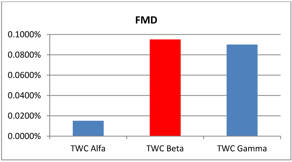
Table 6, Figure 1, Figure 2, Figure 3, Figure 4 show the intensity (the area size beyond the 95% of the scalar field) of each one of the four analyzed epidemics, according to the three TWC scalar fields: α, β and γ.

Table 6. Areas of p > 0.95 according the TWC α, β and γ, in the four analyzed epidemics.

p > 0.95	Foot and Mouth	Chikungunya	London Cholera	Russian Influenza
TWC α	0.0150%	0.225%	0.3050%	0.0125%
TWC β	0.0950%	0.1800%	0.1150%	0.0525%
TWC γ	0.0900%	0.1875%	0.0775%	0.0200%

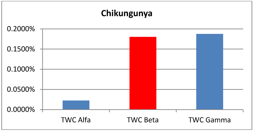
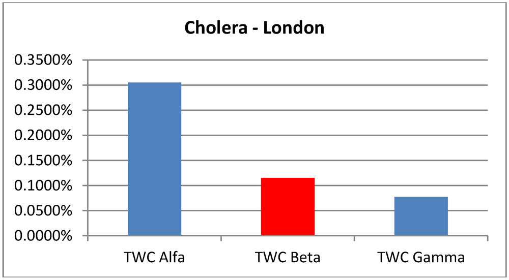
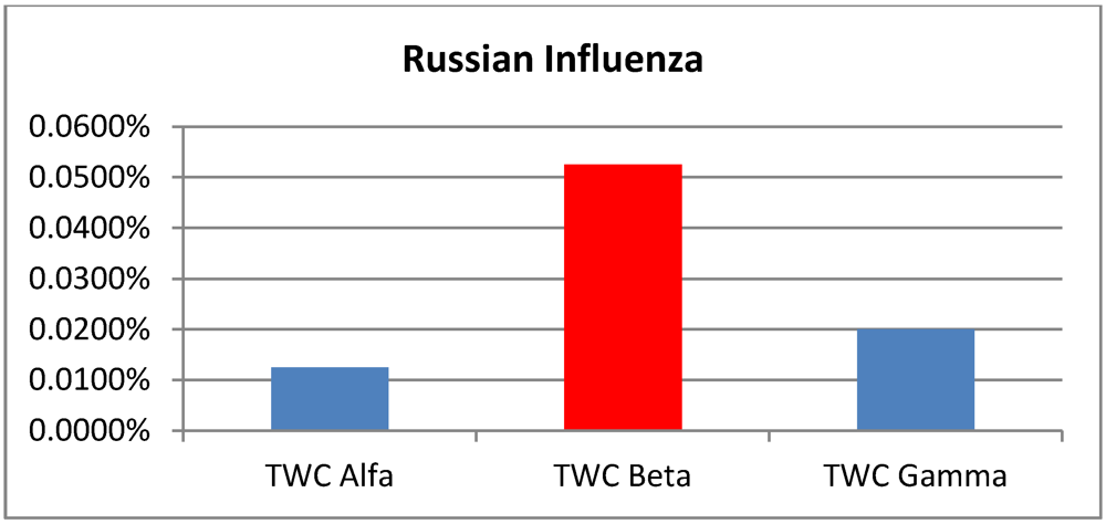
Table 6. Areas of p > 0.95 according the TWC α, β and γ, in the four analyzed epidemics.

p > 0.95	Foot and Mouth	Chikungunya	London Cholera	Russian Influenza
TWC α	0.0150%	0.225%	0.3050%	0.0125%
TWC β	0.0950%	0.1800%	0.1150%	0.0525%
TWC γ	0.0900%	0.1875%	0.0775%	0.0200%

Figure 1. Areas of p > 0.95 according the Topological Weighted Centroid (TWC) α, β and γ, in Food and Mouth Disease.

Figure 1. Areas of p > 0.95 according the Topological Weighted Centroid (TWC) α, β and γ, in Food and Mouth Disease.

Figure 2. Areas of p > 0.95 according the TWC α, β and γ, in Chikungunya epidemics.

Figure 2. Areas of p > 0.95 according the TWC α, β and γ, in Chikungunya epidemics.

Figure 3. Areas of p > 0.95 according the TWC α, β and γ, in Cholera epidemics.

Figure 3. Areas of p > 0.95 according the TWC α, β and γ, in Cholera epidemics.

Figure 4. Areas of p > 0.95 according the TWC α, β and γ, in Russian influenza.

Figure 4. Areas of p > 0.95 according the TWC α, β and γ, in Russian influenza.

From these results we can make some estimation about the next future step of the four epidemics:

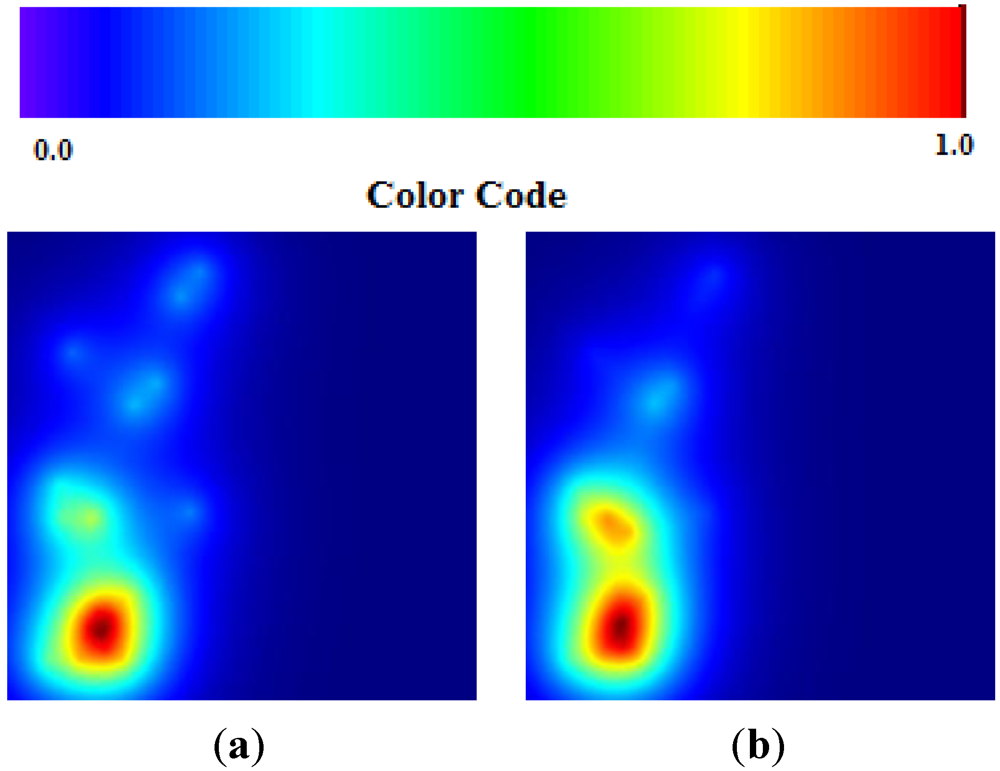
• Data about Foot and Mouth disease were collected when the epidemics were in the first week, before reaching their peak. Despite this, α is small and β is big, as the epidemics would have already reached its peak and as the hot area of its diffusion would have remained stable in the next step (γ is high). See Figure 5(a,b). This discrepancy can be explained by the fact that at variance with the other three examples of epidemics, FMD evolution and spread depend basically from the wind action, since there is no direct contact between animals living in distinct farms. Wind therefore represents another instable variable which probably is not taken into account by our algorithm.
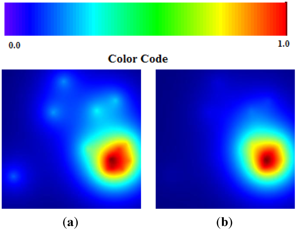
• Data about Chikungunya fever were collected in the main phase of outbreak development. This correspond quite well to the algorithm solution (α is small and β is big). The estimation is a further increase of the hot area in the next future step (γ is bigger than β) (see Figure 6(a,b)).
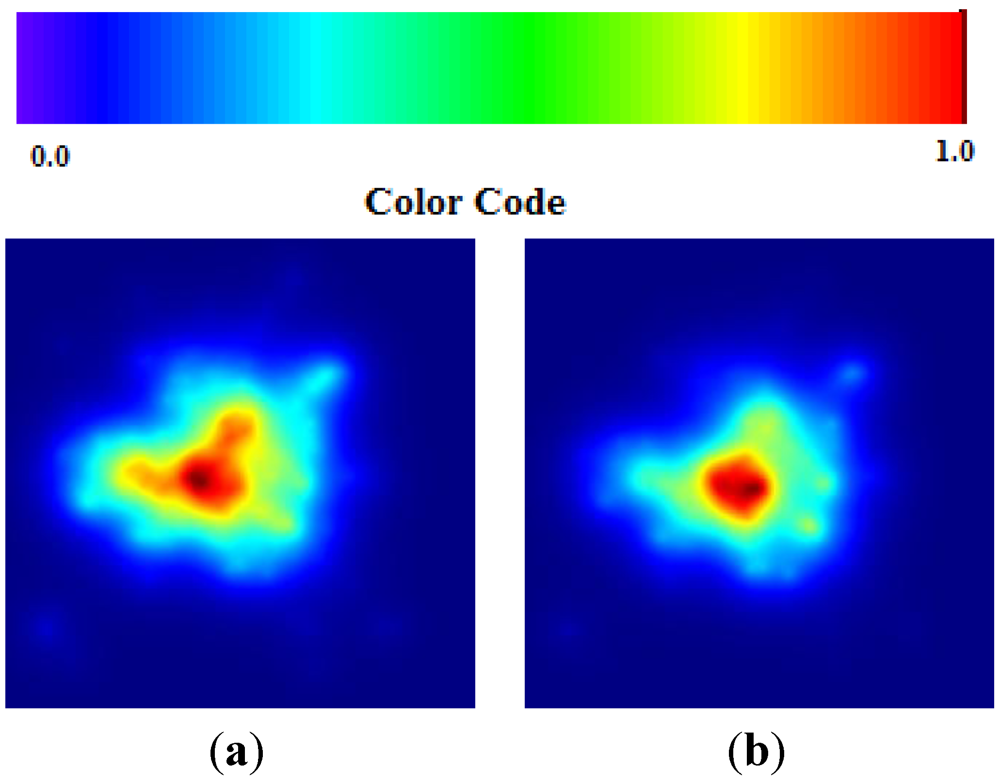
• Data about Cholera correspond to the end of the epidemic outbreak. The values of TWC parameter are consistent with a final state of evolution since α is huge and β and γ become increasingly smaller (see Figure 7(a,b)).
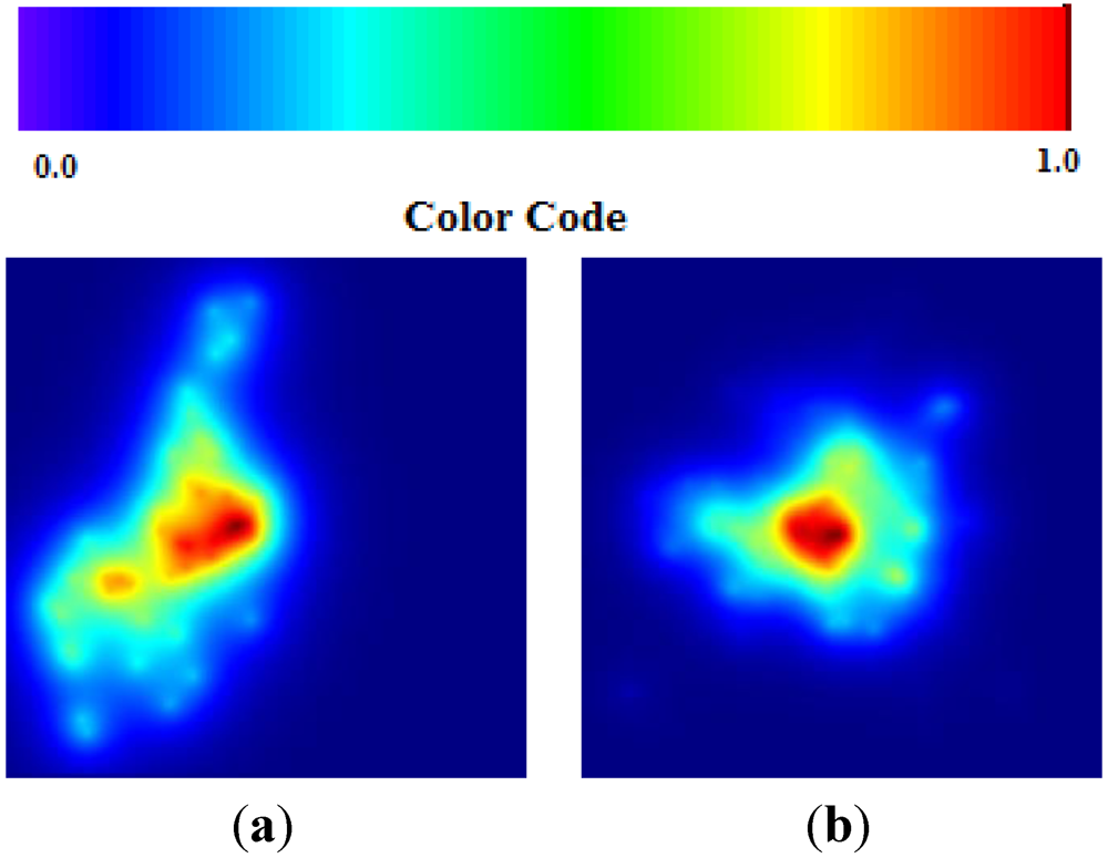
• The data set of Russian flu reflects basically an early phase of development in quantitative terms (number of cases in each location) but a peak for the epidemics in qualitative terms (number of locations). The values of TWC parameters correspond to this evolution phase since β is the biggest. In the next future step the “hot” area of fever is decreased (see Figure 8(a,b)).

In the next section we will see the same estimation about the German Escherichia Coli epidemic, the main purpose of this paper.

Figure 5. (a) FMD TWC (β); (b) FMD TWC(γ).

Figure 5. (a) FMD TWC (β); (b) FMD TWC(γ).

Figure 6. (a) Chikungunya TWC (β); (b) Chikungunya TWC (γ).

Figure 6. (a) Chikungunya TWC (β); (b) Chikungunya TWC (γ).

Figure 7. (a) Cholera TWC (β); (b) Cholera TWC (γ).

Figure 7. (a) Cholera TWC (β); (b) Cholera TWC (γ).

Figure 8. (a) Russian Flu TWC (β); (b) Russian Flu TWC (γ).

Figure 8. (a) Russian Flu TWC (β); (b) Russian Flu TWC (γ).

6. A Special Case of Epidemic Outbreak: The HUS German Epidemics in May–June 2011

6.1.The German Dataset

An unusually high number of cases of hemolytic uremic syndrome (HUS) had been observed in Germany since early May 2011. HUS is a serious and sometimes deadly complication that can occur in bacterial intestinal infections with Shiga toxin (syn. verotoxin) producing Escherichia coli (STEC/VTEC). The complete clinical picture of HUS is characterized by acute renal failure, hemolytic anemia and reduction of circulating platelets number (thrombocytopenia). Typically it is preceded by diarrhea that is often bloody. According to statistics generated by the Robert Koch Institute each year, on average one thousand symptomatic STEC-infections and approximately sixty cases of HUS are reported in Germany, affecting mostly young children under five years of age [27]. In 2010 there were two fatal HUS cases [28]. STEC are of zoonotic origin and can be transmitted directly or indirectly from animals to humans.

Ruminants, especially cattle, sheep, and goats, are considered to be the reservoir. Transmission occurs via the fecal-oral route through contact with animals (or their feces), by consumption of contaminated food or water, or by direct contact from person to person (smear infection). The incubation period of STEC is between two and ten days with a latency period from the beginning of gastrointestinal symptoms to enteropathic HUS of approximately one week.

Table 7 lists the number of cases of HUS or suspected HUS notified to local health departments and communicated by the federal states to the Robert Koch Institute (RKI) by 26 May 2011.

Table 7. Lists of the number of cases of HUS or suspected hemolytic uremic syndrome (HUS) [27,28].

p > 0.95	HUS Cases and Suspected HUS	Cumulative Incidence Cases (per 100,000 Population)
Hamburg	59	3.33
Bremen	11	1.66
Schleswig-Holstein	21	0.74
Mecklenburg-Vorpommern	10	0.61
Hesse	31	0.51
Saarland	5	0.49
Lower Saxony	28	0.35
North Rhine-Weatphalia	31	0.17
Berlin	3	0.09
Baden-Württemberg	8	0.07
Bavaria	5	0.04
Thuringia	1	0.04
Rhineland-Palatinate	1	0.02
Brandemburg	0	0
Saxony	0	0
Saxony-Anhalt	0	0
TOTAL	214	0.26

Table 7. Lists of the number of cases of HUS or suspected hemolytic uremic syndrome (HUS) [27,28].

p > 0.95	HUS Cases and Suspected HUS	Cumulative Incidence Cases (per 100,000 Population)
Hamburg	59	3.33
Bremen	11	1.66
Schleswig-Holstein	21	0.74
Mecklenburg-Vorpommern	10	0.61
Hesse	31	0.51
Saarland	5	0.49
Lower Saxony	28	0.35
North Rhine-Weatphalia	31	0.17
Berlin	3	0.09
Baden-Württemberg	8	0.07
Bavaria	5	0.04
Thuringia	1	0.04
Rhineland-Palatinate	1	0.02
Brandemburg	0	0
Saxony	0	0
Saxony-Anhalt	0	0
TOTAL	214	0.26

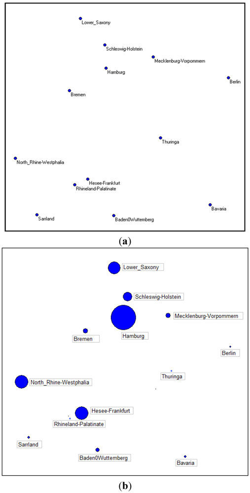
Suspected HUS is included as the syndrome is a process and suspected HUS typically develops over the course of a few days into the full clinical picture. Disease onset (specifically diarrhea) in the 214 patients was detected between 2 and 24 May 2011. A total of 119 (56%) of the cases reported were from four northern federal states (Hamburg, Schleswig-Holstein, Lower Saxony and Bremen). The highest cumulative incidence was recorded in the two northern city states of Hamburg and Bremen. An additional 31 cases occurred in Hesse. Cases began appearing at the start of May and the outbreak swelled to crisis level over the following three weeks, with the city of Hamburg at the epicenter. Initially they were connected to a catering company supplying the cafeterias of a company and a residential institution. Besides the geographic clustering, the age and sex distribution of the cases is conspicuous: of the 214 cases, 186 (87%) are 18 years of age or older (mostly young to middle-aged adults) and 146 (68%) are female. In the notification data for HUS cases from 2006 to 2010, the proportion of adults lay between 1.5% and 10% annually, and the sexes were equally affected.

Cases linked to this outbreak were also from other European countries: On 25 May 2011, Sweden reported through the European Warning and Response System (EWRS) nine cases of HUS, four of whom had travelled in a party of 30 to northern Germany from 8 to 10 May. Denmark reported four cases of STEC infection, two of them with HUS. All cases had a recent travel history to northern Germany. Another two HUS cases with travel history to northern Germany in the relevant period were communicated, one each by the Netherlands and by the United Kingdom.

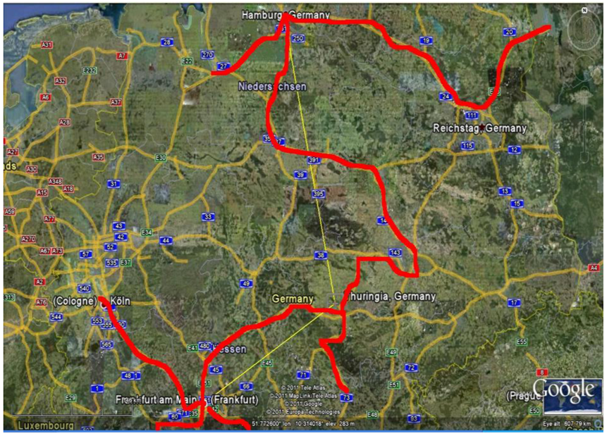
During the outbreak different explanations and hypotheses regarding the source of epidemic outbreak were reported, with a strong impact on public opinion. Preliminary results of a case–control study conducted by Hamburg health authorities demonstrate a significant association between disease and the consumption of raw tomatoes, cucumbers and leafy salads and the attention was focused in the Hamburg area due to the higher density of cases. Two weeks later infected soy sprouts were considered the main problem and a company in Uelzen, a city located roughly 100 km south of Hamburg, became the main suspected source of the infection. This company sells produce mostly in Germany but also exports its products to other European countries and some Asian countries.

On 18 June 2011 the source of the epidemic outbreak was found. The deadly 0104:H4 strain of E. coli that claimed the lives of nearly 40 Germans was found in the northeast of Frankfurt in the Erlenbach stream on the evening of 17 June 2011. The Environment Ministry of the state of Hessen said there were various theories on how the E. coli got into the stream, although a test sample was taken from a nearby sewage plant. While such plants generally have very high hygiene standards, authorities said this could not be ruled out as a possible source.

It has to be noted that during May 2011 data regarding the geographic locations of cases registered were unavailable officially on public WEB site domains. The authors received confidential information regarding the GPS data of the first 13 locations with at least one proved HUS case on May 30 from a person who was attending a congress on environmental toxicity epidemiology in Europe at that time and was in contact with German epidemiologists following the outbreak. Table 8 shows the list of locations.

It has to be noted that the geographic coordinates do not refer specifically to a city involved, but rather to the centroid of the region involved. Only 3 out of 13 locations are exact matches of real occurrences. Figure 9(a) shows the 13 locations on our artificial map; the only data we consider for each location are the latitude and the longitude, 26 numbers for the whole study. Figure 9(b) shows, instead, the same map, considering the frequency of suspected cases in the 13 towns at the time when these data were collected.

Table 8. Geographic location of the first 13 cities/areas with at least one case of HUS.

ID	State	City used	Why used	Lat	Long	Q
1	Hamburg	Hamburg	Exact match	53°33'55''N	10°00'05''E	59
2	Bremen	Bremen	Exact match	53°4'33''N	8°48'27''E	11
3	Schleswig-Holstein	Kiel	Capital	54°19'31''N	10°8'26''E	21
4	Mecklenburg-Vorpommern	Schwerin	Capital	53°38'0''N	11°25'0''E	10
5	Hesse	Frankfurt	Largest city	50°6'37''N	8°40'56''E	31
6	Saarland	Saarbrucken	Capital	49°14'0''N	7°0'0''E	5
7	Lower Saxony	Hanover	Capital	52°22'N	9°43'E	28
8	North Rhine-Weatphalia	Duesseldorf	Capital	51°14'N	6°47'E	31
9	Berlin	Berlin	Exact match	52°30'2''N	13°23'56''E	3
10	Baden-Württemberg	Stuggart	Capital	48°46'43''N	9°10'46''E	8
11	Bavaria	Munchen	Capital	48°31'52''N	11°57'50''E	5
12	Thuringia	Erfurt	Capital	50°59'0''N	11°2'0''E	1
13	Rhineland-Palatinate	Mainz	Capital	50°0'0''N	8°16'16''E	1

Table 8. Geographic location of the first 13 cities/areas with at least one case of HUS.

ID	State	City used	Why used	Lat	Long	Q
1	Hamburg	Hamburg	Exact match	53°33'55''N	10°00'05''E	59
2	Bremen	Bremen	Exact match	53°4'33''N	8°48'27''E	11
3	Schleswig-Holstein	Kiel	Capital	54°19'31''N	10°8'26''E	21
4	Mecklenburg-Vorpommern	Schwerin	Capital	53°38'0''N	11°25'0''E	10
5	Hesse	Frankfurt	Largest city	50°6'37''N	8°40'56''E	31
6	Saarland	Saarbrucken	Capital	49°14'0''N	7°0'0''E	5
7	Lower Saxony	Hanover	Capital	52°22'N	9°43'E	28
8	North Rhine-Weatphalia	Duesseldorf	Capital	51°14'N	6°47'E	31
9	Berlin	Berlin	Exact match	52°30'2''N	13°23'56''E	3
10	Baden-Württemberg	Stuggart	Capital	48°46'43''N	9°10'46''E	8
11	Bavaria	Munchen	Capital	48°31'52''N	11°57'50''E	5
12	Thuringia	Erfurt	Capital	50°59'0''N	11°2'0''E	1
13	Rhineland-Palatinate	Mainz	Capital	50°0'0''N	8°16'16''E	1

Figure 9. (a) Latitude and longitude of the first 13 German towns; (b) Quantity of suspected cases in the first 13 German towns.

Figure 9. (a) Latitude and longitude of the first 13 German towns; (b) Quantity of suspected cases in the first 13 German towns.

6.2. The TWC-α Method and the Real Outbreak

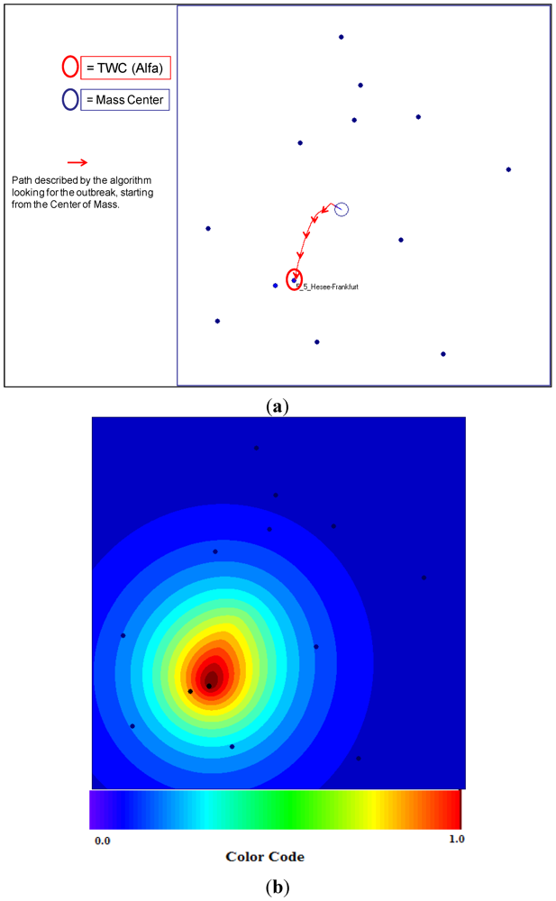
The TWC (α) points start from the center of mass and ends in the vicinity of Frankfurt, which we posited as the source of the outbreak (see Figure 10(a,b)). We remind the reader that the number of cases (frequency) in each location is not considered at all by the algorithm. The TWC algorithm works only considering the geometry of the distribution of the 13 locations.

Figure 10. (a) TWC (α^*) points out the outbreak close to Frankfurt; (b) The scalar field of α_n, the TWSF (α_n).

Figure 10. (a) TWC (α^*) points out the outbreak close to Frankfurt; (b) The scalar field of α_n, the TWSF (α_n).

The center of mass is the point whose summation of the squared distances from the other outbreak locations is minimal and it is also the equilibrium point of the map. In other words, the center of mass is the map position from which the entropy of distribution of the other locations is highest. Therefore looking at the map from this position the other locations appear as the most disordered distribution possible. However, TWC (α) identifies a point on the map where the entropy of the point distribution is lowest; that is, from the TWC (α) position the other 13 locations take the highest value of predictability, the most ordered. In other words, if we locate ourselves at the TWC (α) latitude and longitude, every other location of the map becomes most predictable. 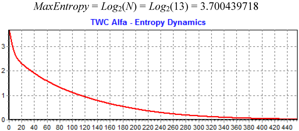Figure 10(a) also shows the path found by the algorithm from the center of mass to the estimated starting point of the epidemic, Figure 10(b) shows the scalar field of the α_n points generated with the TWC (α) method, while Figure 11 shows the dynamics of decreasing the entropy of the system during this search process.

Figure 11. The decreasing of Entropy during the search of TWC (α).

Figure 11. The decreasing of Entropy during the search of TWC (α).

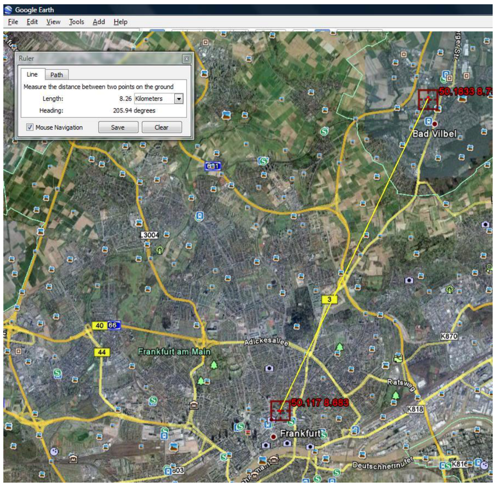
Using Google Earth we found the physical locations of the TWC (α) point. Figure 12 shows its distance from the Erlenbach.

Figure 12. TWC (α), the possible outbreak source, on Google earth at the Long 8.683 and Lat 50.117 and its distance from the Erlenbach stream.

Figure 12. TWC (α), the possible outbreak source, on Google earth at the Long 8.683 and Lat 50.117 and its distance from the Erlenbach stream.

The TWC-α algorithm was found on 29 May 2011 at University of Colorado-Denver, while the outbreak of the HUS epidemics was not publically considered to be in Frankfurt by German authorities. Only on 18 June 2011 did the German authorities name Frankfurt as the second source of the outbreak. If the results of this algorithm had been considered “a possible second opinion” by German epidemiologists on 29 May, a prevention strategy might have been started 20 days prior to the official announcements.

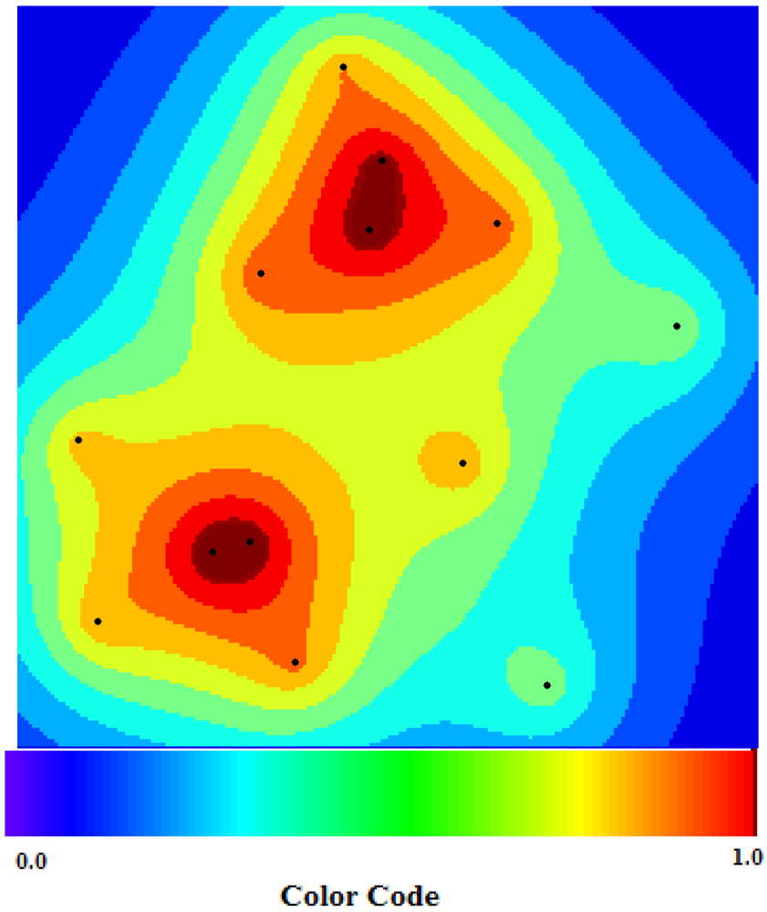
6.3. The TWC-β Map

TWC-β algorithm shows the probability of distribution of the epidemic process at the time of the data collection. Figure 13 shows the map of epidemics divided into two clusters. The Hamburg cluster, in northern Germany, and the Frankfurt cluster, in central Germany. Each cluster consists of multiple areas where the darker and more intensive the red color on the map, the higher the probability of diffusion.

Figure 13. TWC-β scalar field, TWSF (β^*)—the more deep red, the more concentration of epidemics (the deep red zone represents around the 3/1,000 of the whole area).

Figure 13. TWC-β scalar field, TWSF (β^*)—the more deep red, the more concentration of epidemics (the deep red zone represents around the 3/1,000 of the whole area).

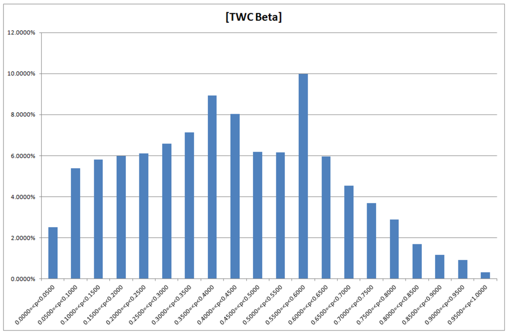
The TWC-β algorithm presents very interesting information:

• The higher probability of epidemics diffusion (p > 0.95) is an area representing 0.32% of total area of the map (see Figure 14); 66% of this area is around Frankfurt, while 34% is in the Hamburg cluster. The intensity of the scalar field was segmented into 20 levels; the 20th is the area where the intensity is largest so the probability of new events should be higher (p > 0.95).

Figure 14. Probability of the epidemics in TWC-β map, in relation to the global areas of the map (20 bins).

Figure 14. Probability of the epidemics in TWC-β map, in relation to the global areas of the map (20 bins).

This means that, according to the TWC-β algorithm, a rapid and intense diffusion of the epidemic would take place in the Frankfurt cluster, while a large and wide diffusion of the same epidemic would happen in the Hamburg cluster. This “non-temporal” prediction is meaningful because the color map of TWC-β (see again Figure 13) reflects exactly the number of cases at the moment of the data collection (see Table 7, and we note that the algorithm does not and did not consider frequency of cases to generate the map).

Using a different methodology and different data, in space and in time, a recent research article [29] shows the network of the diffusion of the HUS epidemic. This network is also divided into two independent hubs starting from the estimated outbreak. Even if one might think that the outbreak predictions in this case were wrong, the hypothesis of two independent clusters to explain the HUS dynamics was nevertheless correctly obtained by our methods. In other words, TWC-β algorithm, using only the latitude and the longitude of the first 13 places where the HUS epidemic was observed, rebuilt a suitable probability map of the HUS diffusion, days before the two locations of the outbreak were announced.

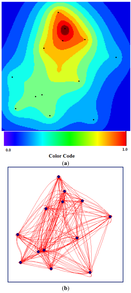
6.4. The TWC-γ Map

The TWC-γ map approximates the distribution of the epidemics, considering the possible diffusion paths rebuilt by the TWC algorithm (see Figure 15(a)). Figure 15(a) is generated by Figure 15(b). The closer a generic point on the map is to the paths, the more probable the diffusion of the epidemics at that point. Figure 15(a,b), in fact, explains (and predicts) the intensity of the diffusion of the HUS epidemic around the Hamburg cluster. And this was what really happened from 29 May to 18 June 2011.

Figure 15. (a) TWC-γ Map where the darker the red, the higher the concentration of epidemics (the darkest red zone represents approximately 1/1,000 of the whole area). (b) TWC-γ rebuilt all the possible paths among the 13 locations.

Figure 15. (a) TWC-γ Map where the darker the red, the higher the concentration of epidemics (the darkest red zone represents approximately 1/1,000 of the whole area). (b) TWC-γ rebuilt all the possible paths among the 13 locations.

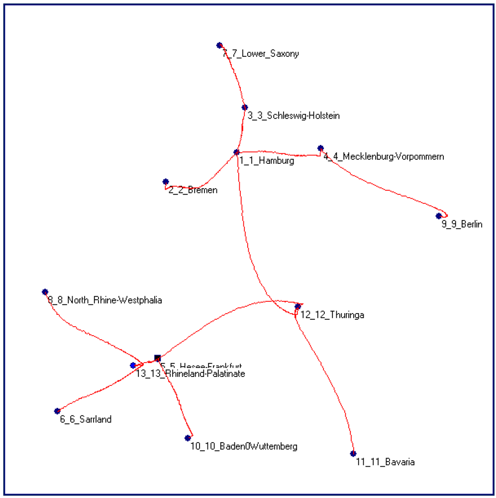
Figure 16 shows the Minimum Spanning Tree (MST) of the complete and regular graph presented in the Figure 6(b), or the most probable path of the epidemic diffusion starting from Frankfurt (the black square point). If we compare the MST of Figure 16 with the real road network of Germany in the same areas (Figure 17, see the red line), the similarity between the two networks is astonishing, particularly if we consider that the nonlinear MST generated by the TWC-γ has no knowledge of any geographical information about the German road system.

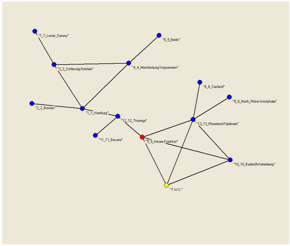
Figure 18 is also a consequence of Figure 16. It is a topological representation of the Maximally Regular Graph (MRG) of the TWC-γ paths. MRG is a special type of graph able to add to the basic MST the most fundamental circuits involved in the original matrix of the non-Euclidean distances from which nonlinear MST is generated (see [30]).

The graph in Figure 18 is of interest for at least three reasons:

• It shows two independent circuits (clicks). The first includes Hamburg, Schleswig-Holstein and Mecklenburg-Vorpommern, and the second includes Frankfurt, the TWC (α) point, and Rhineland-Palatinate and Baden. These two circuits, by means of a feedback loop, should be the main engines of the HUS epidemics, according to the TWC-γ.
• Frankfurt is, in this case, the center of the graph (see Figure 18, the red point).
• Hamburg, Thuringa and Frankfurt are the nodes with a maximum of “betweeness”.

This real world example shows that TWC algorithm is able to trace, with high accuracy, the location of the dynamics of the spread of the German E. coli outbreak with a limited amount of information, even when the information is not precise.

Figure 16. The Diffusion Paths rebuilt by the TWC-γ Algorithm.

Figure 16. The Diffusion Paths rebuilt by the TWC-γ Algorithm.

Figure 17. The real roads, in red, connecting the German towns involved into the epidemics.

Figure 17. The real roads, in red, connecting the German towns involved into the epidemics.

Figure 18. The M.R.G of the paths found using the TWC-γ Algorithm.

Figure 18. The M.R.G of the paths found using the TWC-γ Algorithm.

6.5. Comparison with the Other Algorithms

At the time of the writing of this paper we know that the real outbreak of the German HUS is located near Frankfurt. Consequently, we have compared the solutions proposed by the TWC with the estimation of other algorithms considered in this paper.

Table 9 shows the results of the comparison according to the usual indices. The TWC (α) again outperforms the other algorithms.

Table 10 shows the updated average rank of the algorithms performances. This synthesis of the general performances of all the algorithms in the five tests is quite similar to the results previously shown.

Table 9. Algorithms comparison about German Escherichia Coli.

German Escherichia Coli
Algorithm	Distance from Outbreak	Sensitivity	Specificity	Search Area	Rank
TWC Alfa	1.0700%	97.6000%	99.8675%	0.0105%	1
NES	0.7600%	93.5000%	99.9700%	0.0300%	2
Rossmo	0.7600%	91.3500%	99.9675%	0.0350%	3
LVM	0.7600%	93.6100%	99.9725%	0.0400%	4
Mex Prob	4.4300%	93.6000%	99.8475%	0.3200%	5

Table 9. Algorithms comparison about German Escherichia Coli.

German Escherichia Coli
Algorithm	Distance from Outbreak	Sensitivity	Specificity	Search Area	Rank
TWC Alfa	1.0700%	97.6000%	99.8675%	0.0105%	1
NES	0.7600%	93.5000%	99.9700%	0.0300%	2
Rossmo	0.7600%	91.3500%	99.9675%	0.0350%	3
LVM	0.7600%	93.6100%	99.9725%	0.0400%	4
Mex Prob	4.4300%	93.6000%	99.8475%	0.3200%	5

Table 10. The updated average rank of each algorithm in the five tests.

Algorithm	FMD	Chikunguya	London Cholera	Russian Influenza	German HUS	Rank Average
TWC Alfa	1	1	1	2	1	1.20
NES	3	3	4	1	2	2.60
Rossmo	2	2	5	5	3	3.40
LVM	4	4	3	4	4	3.80
Mex Prob	5	5	2	3	5	4.00

Table 10. The updated average rank of each algorithm in the five tests.

Algorithm	FMD	Chikunguya	London Cholera	Russian Influenza	German HUS	Rank Average
TWC Alfa	1	1	1	2	1	1.20
NES	3	3	4	1	2	2.60
Rossmo	2	2	5	5	3	3.40
LVM	4	4	3	4	4	3.80
Mex Prob	5	5	2	3	5	4.00

6.6. TWC (γ) and German HUS Dynamics

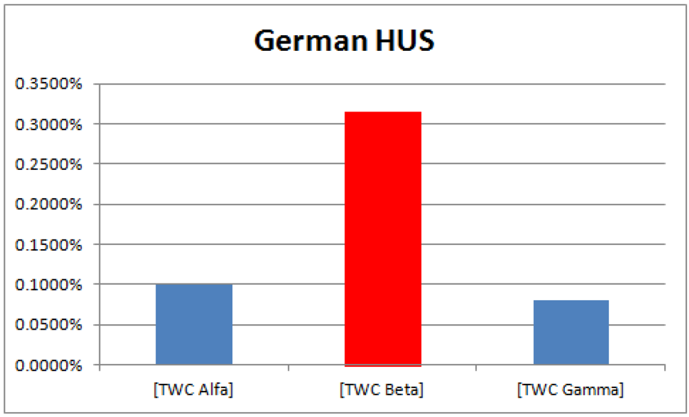
When we compare the size of the hot areas (p > 0.95) according to estimations in TWC α, β and γ (see Figure 19), we note that German HUS at the end of May 2011 was caught at the peak of its diffusion (TWC β shows the biggest area), after a fast and big diffusion from the initial outbreak (TWC α area is not small). Because TWC (γ) area is much smaller than the others, we have to conclude that this epidemic was reducing its impact at the beginning of June.

These estimations have shown to be in accordance with the real development of this epidemic.

Figure 19. German HUS: estimations of the hot areas of diffusion of the epidemic according to TWC α, β and γ.

Figure 19. German HUS: estimations of the hot areas of diffusion of the epidemic according to TWC α, β and γ.

7. Oahu (Hawaii): How to Predict 3 Months before the Intensity of a Food Epidemic

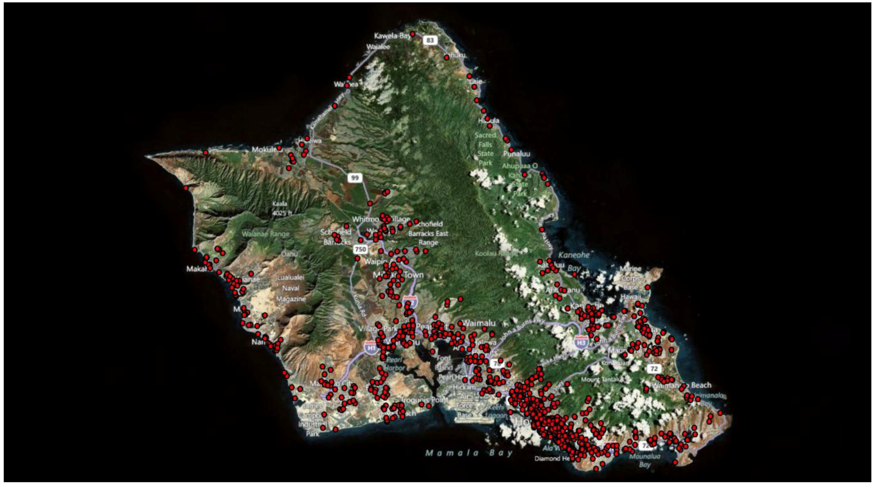
In 2010, Oahu (Hawaii) data from a food epidemic (1,245 cases) were collected systematically for 12 months. We have received this dataset from Al Bronstein, director of the Rocky Mountain Poison Center. Figure 20 shows the geographical distribution of cases of the Oahu epidemic and Table 11 shows the distribution of the new cases each month of 2010.

Figure 20. The geographic distribution of the 1,245 cases of the food epidemic in Oahu (year 2010).

Figure 20. The geographic distribution of the 1,245 cases of the food epidemic in Oahu (year 2010).

Table 11. 1,245 cases of food epidemic in 2010 at Oahu (Hawaii).

Oahu 2010: Number of Cases Each Month
Jan	108
Feb	109
March	114
April	98
May	79
June	79
July	93
August	109
Sept	92
Oct	134
Nov	114
Dec	108

Table 11. 1,245 cases of food epidemic in 2010 at Oahu (Hawaii).

Oahu 2010: Number of Cases Each Month
Jan	108
Feb	109
March	114
April	98
May	79
June	79
July	93
August	109
Sept	92
Oct	134
Nov	114
Dec	108

Table 12. Predictive correlation between TWC (Gamma) and TWC (Beta) with different Delta.

	Gamma(n)=Beta(n) Delta=0
Time Steps	n = 0	n = 1	n = 2	n = 3	n = 4	n = 5	n = 6	n = 7	n = 8	n = 9	n = 10	n = 11	Linear Correlation
Months	Jan	Feb	March	April	May	June	July	August	Sept	Oct	Nov	Dec
Beta(n)	0.1925%	0.1000%	0.1575%	0.1275%	0.2450%	0.1600%	0.1000%	0.0575%	0.2525%	0.0625%	0.0925%	0.0575%	0.28
Gamma(n)	0.1075%	0.0500%	0.1275%	0.1150%	0.1350%	0.3025%	0.0950%	0.0450%	0.0925%	0.1250%	0.1100%	0.0900%
	Gamma(n)=Beta(n+1) Delta=1
Time Steps	n = 0	n = 1	n = 2	n = 3	n = 4	n = 5	n = 6	n = 7	n = 8	n = 9	n = 10	n = 11	Linear Correlation
Months	Jan	Feb	March	April	May	June	July	August	Sept	Oct	Nov	Dec
TWC Beta	0.1925%	0.1000%	0.1575%	0.1275%	0.2450%	0.1600%	0.1000%	0.0575%	0.2525%	0.0625%	0.0925%	0.0575%	−0.24
TWC Gamma	0.1075%	0.0500%	0.1275%	0.1150%	0.1350%	0.3025%	0.0950%	0.0450%	0.0925%	0.1250%	0.1100%	0.0900%
	Gamma(n)=Beta(n+2) Delta=2
Time Steps	n = 0	n = 1	n = 2	n = 3	n = 4	n = 5	n = 6	n = 7	n = 8	n = 9	n = 10	n = 11	Linear Correlation
Months	Jan	Feb	March	April	May	June	July	August	Sept	Oct	Nov	Dec
TWC Beta	0.1925%	0.1000%	0.1575%	0.1275%	0.2450%	0.1600%	0.1000%	0.0575%	0.2525%	0.0625%	0.0925%	0.0575%	−0.22
TWC Gamma	0.1075%	0.0500%	0.1275%	0.1150%	0.1350%	0.3025%	0.0950%	0.0450%	0.0925%	0.1250%	0.1100%	0.0900%
	Gamma(n)=Beta(n+3) Delta=3
Time Steps	n = 0	n = 1	n = 2	n = 3	n = 4	n = 5	n = 6	n = 7	n = 8	n = 9	n = 10	n = 11	Linear Correlation
Months	Jan	Feb	March	April	May	June	July	August	Sept	Oct	Nov	Dec
TWC Beta	0.1925%	0.1000%	0.1575%	0.1275%	0.2450%	0.1600%	0.1000%	0.0575%	0.2525%	0.0625%	0.0925%	0.0575%	0.44
TWC Gamma	0.1075%	0.0500%	0.1275%	0.1150%	0.1350%	0.3025%	0.0950%	0.0450%	0.0925%	0.1250%	0.1100%	0.0900%
	Gamma(n)=Beta(n+4) Delta=4
Time Steps	n = 0	n = 1	n = 2	n = 3	n = 4	n = 5	n = 6	n = 7	n = 8	n = 9	n = 10	n = 11	Linear Correlation
Months	Jan	Feb	March	April	May	June	July	August	Sept	Oct	Nov	Dec
TWC Beta	0.1925%	0.1000%	0.1575%	0.1275%	0.2450%	0.1600%	0.1000%	0.0575%	0.2525%	0.0625%	0.0925%	0.0575%	−0.16
TWC Gamma	0.1075%	0.0500%	0.1275%	0.1150%	0.1350%	0.3025%	0.0950%	0.0450%	0.0925%	0.1250%	0.1100%	0.0900%

Table 12. Predictive correlation between TWC (Gamma) and TWC (Beta) with different Delta.

	Gamma(n)=Beta(n) Delta=0
Time Steps	n = 0	n = 1	n = 2	n = 3	n = 4	n = 5	n = 6	n = 7	n = 8	n = 9	n = 10	n = 11	Linear Correlation
Months	Jan	Feb	March	April	May	June	July	August	Sept	Oct	Nov	Dec
Beta(n)	0.1925%	0.1000%	0.1575%	0.1275%	0.2450%	0.1600%	0.1000%	0.0575%	0.2525%	0.0625%	0.0925%	0.0575%	0.28
Gamma(n)	0.1075%	0.0500%	0.1275%	0.1150%	0.1350%	0.3025%	0.0950%	0.0450%	0.0925%	0.1250%	0.1100%	0.0900%
	Gamma(n)=Beta(n+1) Delta=1
Time Steps	n = 0	n = 1	n = 2	n = 3	n = 4	n = 5	n = 6	n = 7	n = 8	n = 9	n = 10	n = 11	Linear Correlation
Months	Jan	Feb	March	April	May	June	July	August	Sept	Oct	Nov	Dec
TWC Beta	0.1925%	0.1000%	0.1575%	0.1275%	0.2450%	0.1600%	0.1000%	0.0575%	0.2525%	0.0625%	0.0925%	0.0575%	−0.24
TWC Gamma	0.1075%	0.0500%	0.1275%	0.1150%	0.1350%	0.3025%	0.0950%	0.0450%	0.0925%	0.1250%	0.1100%	0.0900%
	Gamma(n)=Beta(n+2) Delta=2
Time Steps	n = 0	n = 1	n = 2	n = 3	n = 4	n = 5	n = 6	n = 7	n = 8	n = 9	n = 10	n = 11	Linear Correlation
Months	Jan	Feb	March	April	May	June	July	August	Sept	Oct	Nov	Dec
TWC Beta	0.1925%	0.1000%	0.1575%	0.1275%	0.2450%	0.1600%	0.1000%	0.0575%	0.2525%	0.0625%	0.0925%	0.0575%	−0.22
TWC Gamma	0.1075%	0.0500%	0.1275%	0.1150%	0.1350%	0.3025%	0.0950%	0.0450%	0.0925%	0.1250%	0.1100%	0.0900%
	Gamma(n)=Beta(n+3) Delta=3
Time Steps	n = 0	n = 1	n = 2	n = 3	n = 4	n = 5	n = 6	n = 7	n = 8	n = 9	n = 10	n = 11	Linear Correlation
Months	Jan	Feb	March	April	May	June	July	August	Sept	Oct	Nov	Dec
TWC Beta	0.1925%	0.1000%	0.1575%	0.1275%	0.2450%	0.1600%	0.1000%	0.0575%	0.2525%	0.0625%	0.0925%	0.0575%	0.44
TWC Gamma	0.1075%	0.0500%	0.1275%	0.1150%	0.1350%	0.3025%	0.0950%	0.0450%	0.0925%	0.1250%	0.1100%	0.0900%
	Gamma(n)=Beta(n+4) Delta=4
Time Steps	n = 0	n = 1	n = 2	n = 3	n = 4	n = 5	n = 6	n = 7	n = 8	n = 9	n = 10	n = 11	Linear Correlation
Months	Jan	Feb	March	April	May	June	July	August	Sept	Oct	Nov	Dec
TWC Beta	0.1925%	0.1000%	0.1575%	0.1275%	0.2450%	0.1600%	0.1000%	0.0575%	0.2525%	0.0625%	0.0925%	0.0575%	−0.16
TWC Gamma	0.1075%	0.0500%	0.1275%	0.1150%	0.1350%	0.3025%	0.0950%	0.0450%	0.0925%	0.1250%	0.1100%	0.0900%

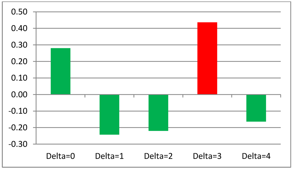
We set up a first validation test about the predictive capability of TWC Gamma as we have hypothesized in Chapter 6 and have independently applied TWC Beta and TWC Gamma to the data of each month. Then, we measured the linear correlation between the sensitivity of the more intensive scalar field of TWC Beta and TWC Gamma (s(x) > 0.9, where x is between 0 and 1). If we hypothesize that TWC Gamma works as a fuzzy estimation of how epidemic intensity will be in the next temporal steps, then we have to compare the highest sensitivity of TWC Beta in the month (n + Delta, Delta = {0,1,2,…,11}) with the highest sensitivity that TWC Gamma estimates at the time (n).

Table 12 shows five comparisons with different values of Delta (0, 1, 2, 3, 4).

It is quite evident that TWC (Gamma) is able to estimate in an acceptable way the high intensity of diffusion of the food epidemic three months in advance (see Figure 21).

Figure 21. Linear Correlation between the Highest Epidemic Intensity in TWC Beta and TWC Gamma Scalar Fields, With Different Temporal Steps.

Figure 21. Linear Correlation between the Highest Epidemic Intensity in TWC Beta and TWC Gamma Scalar Fields, With Different Temporal Steps.

Obviously we do not consider this test as a complete validation of the prediction capability of TWC Gamma. We need to plan a more extensive and deep validation protocol to verify the plausibility of what we are assuming. This short and non-representative test is only the first positive step of process that needs to be improved in future work.

8. Discussion

Infectious diffusive diseases may present themselves with complex temporal and spatial patterns difficult to discern. These diseases, as opposed to chronic diseases, are somewhat unique because exposure and outcome are the same, i.e., the infected person or animal. This leads to non-linear dynamics that make analysis and prediction of infections in a population very challenging.

Each year, millions of people worldwide die from infectious diffusive diseases such as malaria, tuberculosis, dengue fever, West Nile virus, etc. Government agencies seek efficient mathematical models better able to provide insight into the dynamics of disease epidemics and to help officials make decisions about public health policy.

The basic premise in outbreak investigation is that the process does not occur randomly. Sometimes specific patterns by themselves provide clues about the transmission modality in place. A rapid increase in the number of cases over a very short period of time, for example, suggests a point-source epidemic where a large number of subjects are exposed to a common source of the disease-causing agent at the same time. Such a pattern is often seen with food-borne or water-borne diseases or a highly virulent infectious agent. A case or two followed by a gradual increase in the frequency of disease suggests a propagated epidemic where there is an animal-to-animal transmission of an infectious agent either directly, through fomites or insect vectors. In both cases however the precise identification of the starting place of the epidemics can be a difficult challenge.

Theoretically, given a distribution of points in a specific environment and a certain number of constraints related to types of physical characteristics of the territory, such as different types of possible trips and metrics (travel time, effort, or cost), there is an optimal solution that minimizes the distance between points and their source. However, computationally, it is an almost impossible task to define, requiring the enumeration of every possible combination, which is known as an NP-hard problem. Consequently in practice, approximate, though possibly sub-optimal, solutions are obtained through a variety of methods. “Location theory” attempts to find an optimal location for any particular distribution of activities, population, or events over a region according to a specific criterion, and is therefore one of the central issues in geography. In the case of outbreaks source identification, one can reverse the logic. Given the distribution of points of interest, the theory could be applied to estimate a central location from which travel distance or time is minimized. Epidemic models try to describe the spread of infectious diseases in populations. More and more, these models are being used for predicting, understanding and developing control strategies. In realistic epidemic models, a key issue to consider is the representation of the contact process through which a disease is spread, and network models have arisen as good candidates predicting which cities are sources for the epidemic and understanding the path of recurrent traveling waves may help us to design optimal surveillance and control strategies.

The principle on which we based our approach is the separation of the topographical element from the frequency (incidence) of the event. This per se constitutes a paradigm shift in modern epidemiology. The main advantage of this approach is that algorithms like TWC can be used in the initial stage of an epidemic, even when not all cases are known. Subsequently, we can match topographic distribution with frequency in a gradient descent to identify the location on which distance and event frequency are shortest. This might lead to a significant contribution to improving the quality of infection control.

It is quite clear that the conclusions drawn from geographic mapping depend on the accuracy and validity of the datasets, and to enable repetition of our analysis we would recommend the use of high quality, credible data. However, it is remarkable that the TWC algorithm seems very robust despite imprecise information regarding the exact localization of cases in the early stage of the HUS epidemic. This is suggested by the accuracy with which the TWC (α^*) predicted “backwards” or retrodictively, the source of the epidemics, despite the program (and also the authors) not being told of its nature or location (Hamburg), which was, at the time of analysis, unknown and to be located six-hundred km distant from the second source (Frankfurt). It is not irrational therefore to believe that this approach could be applied in real world situations during future epidemic outbreaks to describe and better understanding the spatial-temporal features of infection risk and spread.

There are a number of points of strength in this paper: First of all the TWC algorithm is logically rigorous and gives explicit assumptions on the source of dynamic process. Secondly the validation relies on five notorious data sets with a large number of cases, all published in the literature in which the source of the epidemic spread has been unequivocally proved. Thirdly the performance of the algorithm has been contextualized in the field of other algorithms used for geographic profiling. The comparison with these benchmarking systems has required the development of a sound methodology based on multiple parameters. This per se represents a real progress in this field.

The resulting TWC alpha is found to be the top performer among the four algorithms selected for comparison, which are in our view the best available today in all four experiments as regards the distance from outbreak in three out of four, and second in one out of four experiments (Russian flu) as regards the searching area.

In addition, the TWC algorithm provides other parameters very useful in handling epidemic outbreak information: the TWC beta represents the actual intensity of epidemics and TWC gamma represents the future dynamic trajectory of epidemics.

Despite our consistent findings, we are aware of one principal limit of this study. Four epidemics represent a good proof of concept but may not be representative of all epidemics. Therefore our method will need careful verification and validation both from other well-documented outbreaks and during the early phases of new outbreaks, both in human and animal settings.

Our findings should also stimulate attention to the contribution of mathematical modeling in improving the precision of bio-medical sciences. Our analysis shows how a system with complex systems mathematics can provide alternatives to classical methods. In addition, this is a powerful tool for the investigation of the early stages of an epidemic, and might constitute the basis of new simulation methods to understand the process through which an infectious disease is spread.

9. Conclusions

TWC algorithms, as presented in this paper, represent a first step of a new theory of the semantics of the space. We know that many other steps are needed to adequately design a complete theory.

This work demonstrates the possibility of reading the semantic information of a distribution of events into a bi-dimensional space in topological terms. Consequently, the probabilistic approaches and the gravitational approaches are neither the best solutions nor are they the only ones.

We seek to integrate the TWC algorithms in future research initiatives following this agenda:

• To include a new algorithm (based on the TWC philosophy) able to identify a set of possible and different outbreaks given one spatial distribution of events.
• To include a third spatial dimension in space analysis, and consequently a new metric able to consider the energy needed to complete a path (and not only the distance).
• The addition of the latitude and the longitude a list of meaningful qualitativeattributes for each event, and to find a way to collectively process all these features.
• The integration of the time flow to the TWC approach in such a way as to explain how the maps change when some attributes of the spatial events change, and which of those attributes could possibly be the cause-effect link between these changes.

TWC algorithms must be integrated into a general theory of semantics of events located in specific space and under specific time constraints.