1. Introduction
Reservoirs are important hydrologic features affecting numerous aspects of the aquatic and riparian environment [
1]. While definitions between pond and reservoir vary regionally and by discipline [
2], here we define reservoir as a water body created through artificial impoundment for the storage and regulation of water. Reservoirs modify downstream sediment loads, water chemistry, and nutrient regimes in complex ways [
3,
4,
5]. Reservoirs capture suspended sediment, nutrients, and pollutants by slowing water velocities and allowing these inputs to drop out of the water column and become stored in the benthos [
6,
7]. Over time, downstream reaches become sediment-starved and exhibit altered geomorphology while the reservoirs in-fill and lose water storage capacity [
8,
9,
10]. The sedimentation, which is commonly rich in nutrients and pollutants, requires ongoing management [
11,
12]. In addition, reservoirs may contribute to downstream nutrient levels if they are managed for recreational fishing and are fertilized to promote algae growth and sustain populations of stocked fish [
13,
14]. Fishery management practices may also include the use of toxicants such as rotenone and antimycin A to control nuisance or undesirable species [
15,
16,
17].
Reservoirs alter downstream flow regimes in complex ways depending on the reservoir water level and hydrologic conditions. When storage capacity is available within a reservoir, water is captured and gradually released, dampening downstream peak flows [
18]. Decreasing flood frequency can disconnect the river from its floodplain, leading to ecological shifts in the riparian zone such as a transition from floodplain species to upland species [
19,
20]. Hydrologic models have demonstrated the important role that small depression storage features [
21] and stormwater detention reservoirs [
22] play in flood response. In contrast, under full-storage conditions, reservoirs act as an impervious surface and rainfall is immediately moved downstream rather than being intercepted and slowed by alternate land cover such as riparian buffers [
23]. During the initial stages of low streamflow conditions, downstream water quantities can be supplemented by stored reservoir water. However, under prolonged drought conditions, dry reservoirs capture water and either delay or altogether prevent flows from moving downstream. In addition, the loss of downstream water quantity due to reservoir evaporation can be substantial [
24].
Reservoirs have a substantial effect on aquatic species [
25]. By fragmenting stream systems, species are isolated from the headwaters, affecting access to breeding grounds, altering genetic diversity, and modifying species abundance and distribution [
26,
27]. Reservoir creation also directly modifies habitat availability by converting a riverine environment to a lacustrine environment thereby decreasing the quantity of available habitat for riverine species. Finally, reservoirs affect aquatic ecology by altering water temperature and dissolved oxygen levels [
28,
29]. For instance, reservoirs that release water from the benthic zone typically send cool and less oxygenated water downstream. In contrast, “top release” reservoirs discharge water from the lake surface and send warm water downstream.
The impacts of large reservoirs, which store from 100,000 m
3 to over 25,000,000,000 m
3 of water, have been well-studied across disciplines such as biology, hydrology, ecology, geography, and engineering [
1,
18,
30,
31,
32,
33]. In contrast, the impacts of small reservoirs, which commonly capture less than 100,000 m
3 of water, are substantially less studied [
31,
32,
33]. Compared to large reservoirs, the localized effects of a single small reservoir can seem innocuous; however, over the past two decades researchers have come to recognize the considerable cumulative impact of several thousand small reservoirs at the landscape scale [
34,
35].
Over the past two decades, advancements in remote sensing and Geographic Information Systems (GIS) technologies have enabled researchers to identify extensive numbers of artificial reservoirs across the United States (U.S.) and demonstrate their importance within hydrologic networks [
31,
36,
37,
38]. However, little is known about the drivers of small reservoir creation or the patterns in their distribution and rate of construction over time. Some historical research has been conducted using archival maps and records to reconstruct the extent of small dam construction within locations such as the eastern U.S. and Scotland [
39,
40]. However, much of this research focuses on historically documented pre-20th century mill dams and does not address recent trends in the numbers of small farm reservoirs, private fishing reservoirs, and municipal stormwater and amenity reservoirs.
U.S. Government programs have provided some documentation of fishing and farm pond creation over time. Federal efforts to promote small farm pond construction began as early as 1872; however, not until the 1930s did these programs make substantial headway in construction efforts [
41]. Starting in the 1930s, programs in the U.S. Fish and Wildlife Service (the Bureau of Sport Fisheries and Wildlife) and the Department of Agriculture (the Soil Conservation Service and the Agricultural Conservation Programs Branch of the Production and Marketing Administration), helped fund private pond construction, provide technical management guidance, and supply fish for stocking purposes [
2,
42]. The 1930s initiatives focused on pond creation for erosion-control and to assist with conversion of land from eroded fields to pasture by providing livestock watering [
39]. By 1952, small reservoirs were being constructed across the U.S. at a rate of 38,000 per year with the assistance of the Soil Conservation Service (an unknown number of additional ponds were created without Federal assistance) [
39]. In 1949, the venerated fisheries scientist, H.S. Swingle, stated that “in the previous 15 years there had been constructed in the U.S. at least 100 times as many ponds as had been constructed during the preceding 200 years” [
39].
Since the 1970s, reservoirs have increasingly been utilized to mitigate stormwater runoff [
43]. Typically, local regulations are enforced only if the increased impervious surface associated with a new development will increase the quantity of stormwater in exceedance of a stipulated minimum threshold (for example, 0.01 m
3/s) [
44]. To mitigate development impacts, local jurisdictions commonly mandate that new developments construct stormwater ponds to capture sediment during the construction process and to later mitigate stormwater runoff and pollution problems downstream. However, these regulations vary widely across the U.S. depending on state and county laws. After construction, the mitigation ponds are commonly considered to be amenity ponds that provide aesthetic value. While stormwater reservoirs can reduce peak flooding, it should be noted that the overall efficiency and effectiveness of these constructions has recently been brought into question [
45,
46].
Despite acknowledgement of the different economic drivers, societal factors, and policies motivating reservoir construction within the U.S., the relative importance of each of these factors and their influence over time and space is not documented. The lack of information about small reservoir creation hampers water managers and policymakers. Information about the age and distribution of dams and reservoirs would help water resource managers assess water quality and quantity impacts over time and at the watershed scale. Assessment and monitoring of stream ecological health in terms of species abundances and distributions would also benefit from temporal information about reservoir distribution and creation. More thorough documentation of reservoir construction dates would also help managers track and maintain even the smallest dams to mitigate against dam failures. Policymakers would benefit from knowing how citizens are using small reservoirs over time and what policies have been most influential in terms of small reservoir creation. Policymakers would also benefit from information about the basin-wide impacts of reservoir creation and the cumulative importance of reservoir creation incentives and ordinances. At the landscape scale, the changing uses of individual small reservoirs are not well understood. On an individual basis, ponds may be modified from privately owned, forested fishing ponds or farm ponds to urban amenity ponds when land is sold to developers and subdivided for suburban uses, however, the extent of this practice is not well documented.
Outside of the U.S., different factors affect pond creation. Within developing nations such as Ghana, Kenya, and Zimbabwe, the proliferation of small reservoirs started later than in the U.S. but has rapidly affected fluvial systems and the landscape over the last two decades [
47,
48,
49]. Growing populations and expanding infrastructure have put increased pressure on scarce water resources, leading to a boom in small reservoir construction for water security. Small reservoirs contribute to the improvement of small farm owner livelihoods, food security, and sustainable agriculture [
50]. International aid programs promote reservoir construction as essential infrastructure, as well. Documenting the extent and impacts of reservoir construction within the U.S. could help inform developing regions about the impacts of various programs, regulations, and private landowner decisions and the trade-offs inherent in landscape-scale small reservoir development.
To examine the roles and patterns of small reservoir construction during the last half of the 20th and beginning of the 21st centuries, we considered four primary questions as part of a case study in the upper and middle Chattahoochee basins within the Southeastern U.S. Georgia Piedmont from 1950 to 2010:
How have small reservoirs contributed to the total inundated surface area?
What was the rate of small reservoir construction?
How has land cover adjacent to small reservoirs changed (agricultural, developed, or forested)?
How have small reservoirs contributed to stream fragmentation?
2. Study Watershed Selection
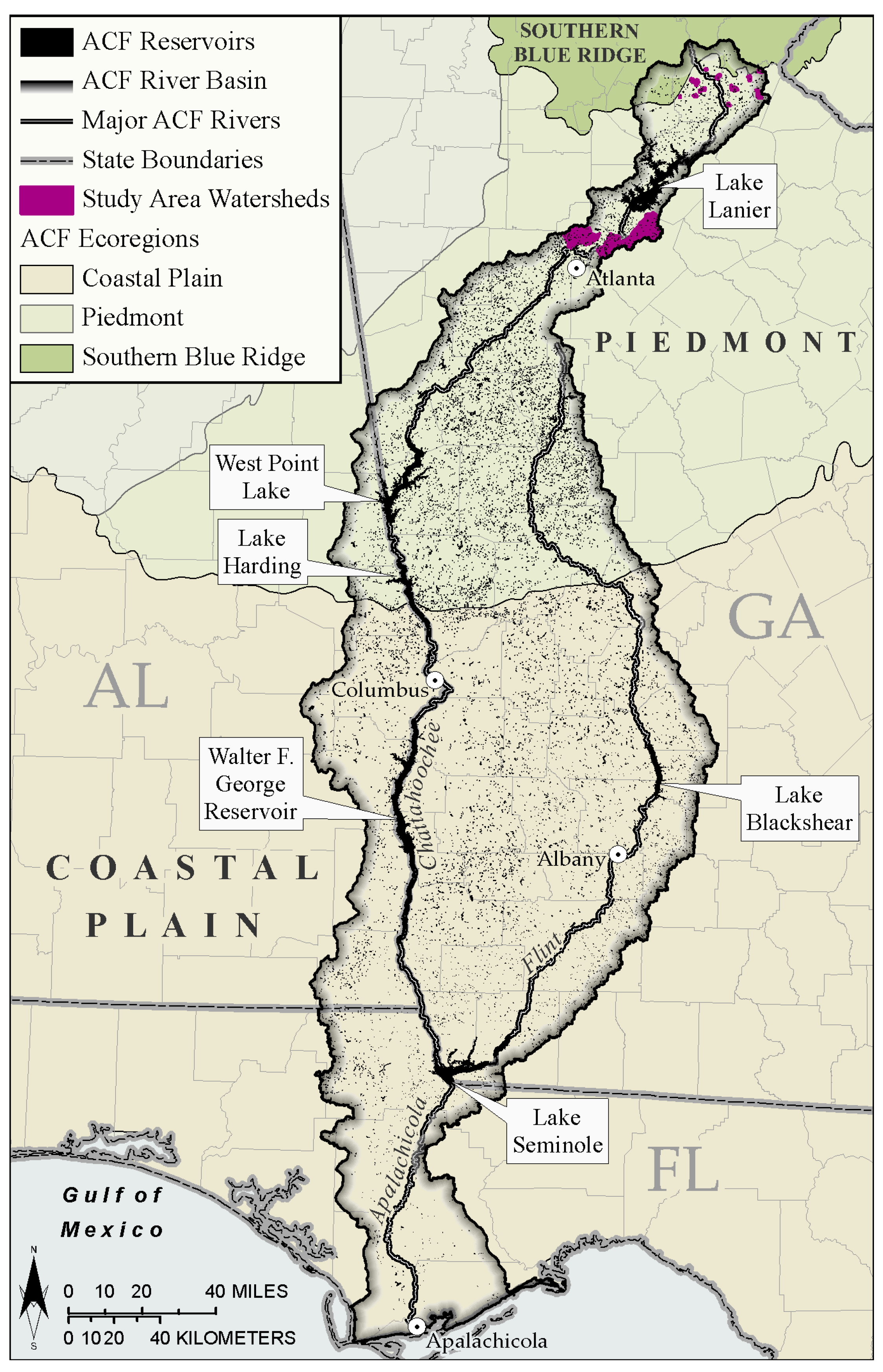
The Apalachicola-Chattahoochee-Flint (ACF) River basin is a 50,000 km
2 watershed that includes portions of three States: Alabama, Florida, and Georgia (
Figure 1). Since 1989 the ACF basin has been at the center of a multi-million dollar “water war” and ongoing litigation over surface-water allocation [
51,
52]. While the area typically receives ample rainfall that is distributed throughout the year (approximately 125 cm annually), the region is also subject to drought [
53,
54]. The ACF basin contains a high number of artificial water bodies with at least 25,000 reservoirs recognized in a recent study [
55]. However, no database exists to monitor these artificial water bodies over time. As a result, building dates, motives for construction, and subsequent uses of reservoirs in the ACF basin remain largely undocumented.
Figure 1.
Map of Apalachicola-Chattahoochee-Flint (ACF) River Basin.
Figure 1.
Map of Apalachicola-Chattahoochee-Flint (ACF) River Basin.
We focused our historical analysis on the upper and middle Chattahoochee basins in the Piedmont ecoregion in the northern part of the larger ACF basin (
Figure 1 and
Figure 2). The Piedmont is an ideal study region for this research because it has few natural lakes [
56,
57] and most lacustrine water bodies identified using aerial imagery can be classified as reservoirs. In addition, the Piedmont’s geologic properties and human history explain why the upper and middle Chattahoochee basins have the highest concentration of reservoirs in the entire ACF [
54]. Geologically, the Piedmont consists of crystalline bedrock overlain by unconsolidated regolith (a thin cover of regolith in steeper areas and up to 30 m of regolith in broad valleys) [
58]. While some groundwater may be obtained directly from the regolith or from bedrock fractures, these sources provide unreliable and commonly inadequate groundwater supplies as the unfractured rock has small pore space, low porosity, and low permeability [
57]. The upper and middle Chattahoochee basins include the Atlanta metropolitan area, one of the fastest growing metropolitan areas in the U.S. [
59]. Between 1973 and 1999, the population of the Atlanta region increased by 96% and every week during this period more than 40 hectares of forest, green space, and farmland were developed for urban uses [
59]. With limited groundwater resources, the growing population is reliant on surface water. To meet demand, local and state governments have initiated various policies to promote reservoir construction and maintenance [
60,
61,
62].
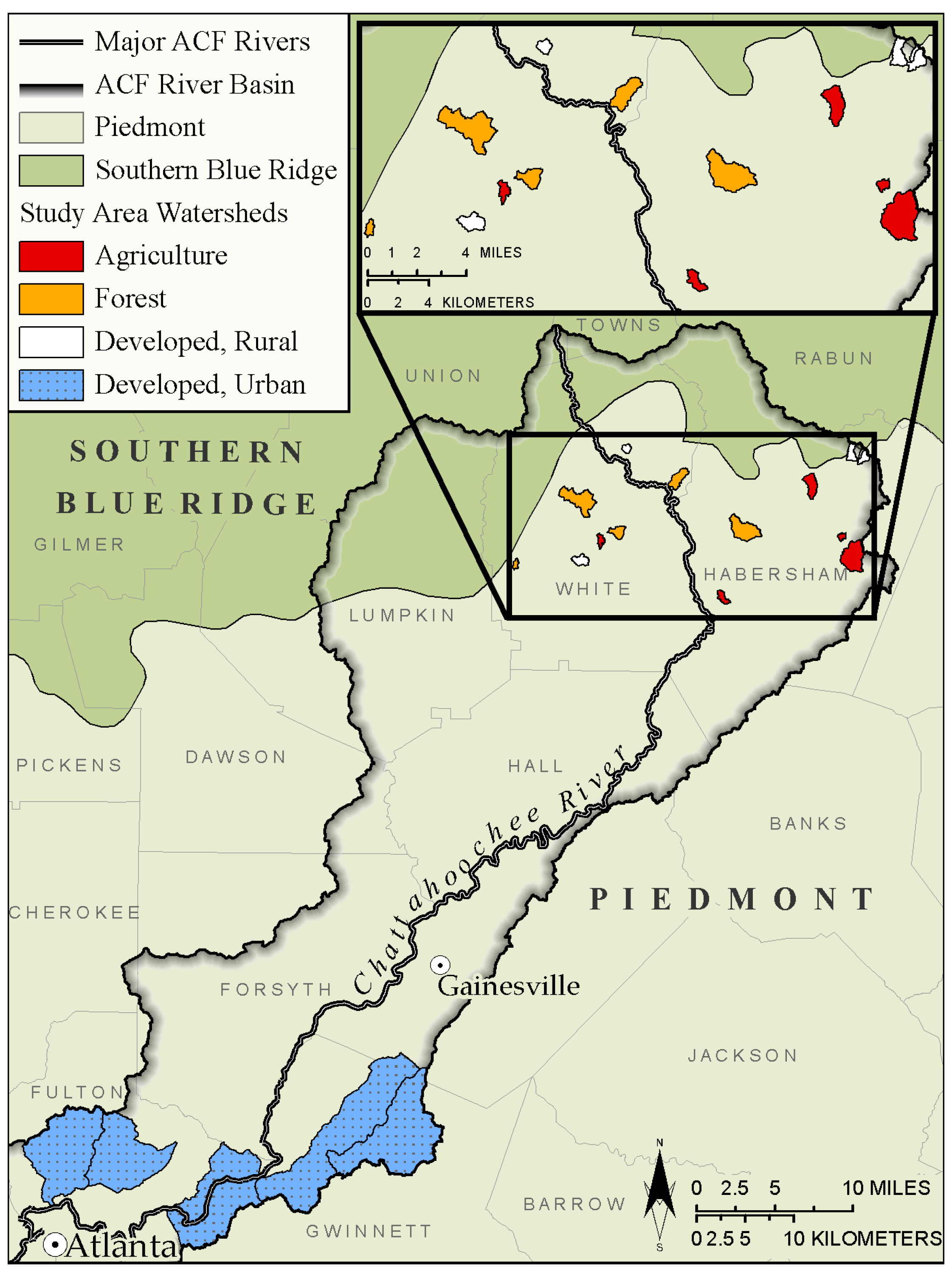
Figure 2.
Map of 20 study area watersheds: five agriculture, five forest, five rural developed, and five urban developed.
Figure 2.
Map of 20 study area watersheds: five agriculture, five forest, five rural developed, and five urban developed.
The upper and middle Chattahoochee basins are advantageous for small reservoir research because their land cover heterogeneity enables comparison of reservoir trends within diverse settings. These basins include forested mountainous regions, agricultural areas, low-intensity rural development, and high-intensity urban development. We focused analyses on watersheds with an abundant quantity of small reservoirs while also considering land cover variety. Specifically, we employed two study site selection methods.
To identify one set of study watersheds we utilized the National Hydrography Dataset HUC12 watershed boundaries [
63]. Among the HUC12 watersheds, we sought areas that met the following criteria: (1) reservoirs were located within the watershed as of 2009 aerial photography; and (2) aerial photography was available for the watershed from 1950 to 2010 at approximately 10-year intervals. Six watersheds were identified in Gwinnett and Fulton Counties that met these criteria and five of these were randomly selected for historical analysis. As of 2010, all five of these watersheds were dominated by high-intensity development and urban land cover.
We determined that use of the relatively larger HUC12 watershed boundaries to examine reservoir patterns in agricultural, forested, and rural areas, would be inappropriate. For example, forested regions generally contain just a few reservoirs that are separated by large expanses of forested land. Use of the larger HUC12 watershed boundaries for forested watersheds would necessitate time-consuming georeferencing of aerial photographs for large swaths of forested land that contains no reservoirs, providing little additional information on reservoir patterns over time. As an alternative, for agricultural, forested, and rural study watersheds we used U.S. Geological Survey (USGS) Southeastern Regional Assessment Project (SERAP) study areas within the Chestatee and Chattahoochee basins in the far northern portion of the ACF [
64]. The SERAP study generated detailed watershed boundaries for this area from the National Elevation Database (NED) for use in ecological flow modeling research [
25].
To examine patterns in reservoir development across a suite of land covers, we selected five agriculture-dominated watersheds, five forest-dominated watersheds, and five rural development-dominated watersheds from the SERAP boundaries using the following criteria: (1) reservoirs were located within the watershed as of 2009 aerial photography; (2) the watershed was dominated by a single land use type and had at least 40% of its land cover within this dominant category based on the 2001 National Land Cover Database (NLCD) [
65]; and (3) the watershed was at least 0.2 km
2 in size. In total, seven agricultural watersheds, 286 forested watersheds, and five rural development watersheds met these criteria. Of these totals, five watersheds were randomly selected from each class for historical analysis.
In total, these two selection methods provided 20 watersheds encompassing a total of 313.21 km
2: five high-intensity urban developed watersheds based on HUC12 boundaries, five agricultural watersheds based on SERAP boundaries, five forested watersheds based on SERAP boundaries, and five rural developed watersheds based on SERAP boundaries (
Figure 2). While the HUC12 watersheds were much larger than the SERAP watersheds (on average, 57 km
2 for HUC12 and only 2 km
2 for SERAP watersheds), this method allowed us to efficiently sample areas that contained the highest quantities of reservoirs while also examining multiple land covers within the region.
3. Land Cover Change Tracking
For all 20 study area watersheds, we collected aerial photography for 10(±3)-year intervals from approximately 1950 to 2010. The sources of photography vary greatly depending on availability for the location and time period. Imagery included U.S. Department of Agriculture (USDA) and USGS historic aerials, USGS National High Altitude Photography (NHAP), USGS Digital Orthophoto Quarter Quads (DOQQ) imagery, and USDA National Aerial Imagery Program (NAIP) imagery (
Table 1).
Imagery was acquired and scanned from the University of Georgia Map Library in Athens, Georgia, downloaded from the USGS EarthExplorer website, or downloaded from the Georgia GIS Data Clearinghouse website.
Imagery from approximately 1950, 1960, 1970, and 1980 were georeferenced in ArcGIS 10 [
66] using 2009 NAIP imagery of 1-m spatial resolution as reference. In total, this amounted to 160 manually georeferenced and rectified images from all four decades and covering all 20 study watersheds. Georeferencing root mean square error (RMSE) did not exceed 4.7 m. Next, the images were visually inspected for each time period and all reservoirs were identified based on shape, tone, and texture. All reservoir boundaries were manually digitized using ArcGIS editor. We created two boundary datasets for each water body during each time period: (1) the inundated or “wetted” surface area; and (2) the total reservoir surface area (including both wetted area and dry reservoir bed).
Table 1.
Historic imagery agency, year, scale, and format.
Table 1.
Historic imagery agency, year, scale, and format.
| Agency | Year | Scale | Format |
|---|
| U.S. Department of Agriculture Historic Aerials | 1950, 1951, 1960, 1972, 1973 | 1:20,000 | Black and white 9 × 9 inch negatives. |
| U.S. Geological Survey Historic Aerials | 1947, 1951 | 1:20,000 | Black and white 9 × 9 inch negatives. |
| U.S. Geological Survey National High Altitude Photography (NHAP) | 1977, 1981 | 1:80,000, 1:58,000 | Black and white, Color infrared. |
| U.S. Geological Survey Digital Ortho Quarter Quads (DOQQ) | 1999 | 1:12,000 | Color infrared. |
| U.S. Department of Agriculture National Aerial Imagery Program (NAIP) | 2009 | 1:12,000 | True color. |
While the land cover category for each of the 20 watershed study areas was assigned as agricultural, forested, rural developed, or urban developed based on the 2001 NLCD dominant value, the classification of each individual reservoir could vary from that of the rest of the watershed and could change over time. For example, an agricultural watershed may contain a forested reservoir in 1950 that later became a developed reservoir by 2010. The adjacent land cover classifications were based on interpretation of reservoir context. Each reservoir was assigned to one of the following classes: forest, agriculture, or developed. For example, the presence of chicken houses, terraced fields, or crop plots indicated an agricultural land cover. In contrast, the presence of a subdivision, adjacent highway roads, or large buildings was indicative of developed land cover.
Using the ArcGIS select by location tool, reservoir shapefiles for each time period were extracted to calculate the number of reservoirs in place or abandoned per time period. Finally, to evaluate the impact of small reservoirs on stream fragmentation, polygons of the full reservoir boundary were intersected with the USGS National Hydrography Dataset (NHD) Flowline shapefile and reservoirs were categorized as either on-stream or off-stream.
4. Results
The order-of-magnitude size differences between watersheds of the two development categories (57 km2 average size for urban and 2 km2 average size for rural) prohibits direct comparison of reservoir quantities across study watersheds. In addition, data normalization across watersheds by conversion to reservoir densities is not possible because the selection method excluded watersheds without reservoirs. Therefore, results of adjacent land cover analyses are provided and discussed separately for each watershed classification category (agriculture, forest, rural developed, and urban developed), rather than considered cumulatively across all.
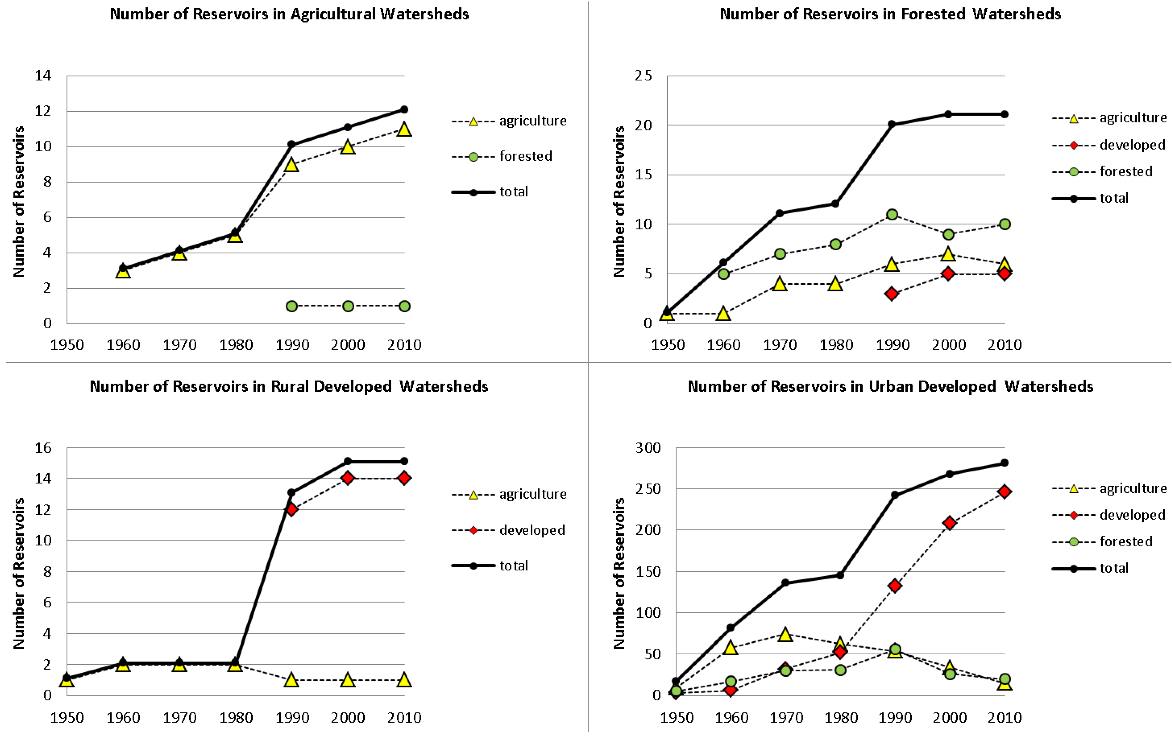
The quantity of reservoirs increased from 1950 to 2010 in all study areas with a total increase from 19 to 329 reservoirs (
Table 2). This pattern was true across all watershed categories with the number of agricultural watershed reservoirs increasing from three to 12, forested watershed reservoirs increasing from one to 21, rural developed watershed reservoirs increasing from one to 15, and urban developed watershed reservoirs increasing from 17 to 281 (
Figure 3).
Table 2.
Reservoir quantity and surface area statistics (h) in all watersheds, 1950–2010.
Table 2.
Reservoir quantity and surface area statistics (h) in all watersheds, 1950–2010.
| Year | 1950 | 1960 | 1970 | 1980 | 1990 | 2000 | 2010 |
|---|
| Number of Reservoirs | 19 | 92 | 153 | 164 | 285 | 315 | 329 |
| Total Surface Area | 50.62 | 140.77 | 186.85 | 187.67 | 278.20 | 299.23 | 298.56 |
| Minimum Surface Area | 0.12 | 0.04 | 0.05 | 0.05 | 0.03 | 0.03 | 0.03 |
| Maximum Surface Area | 30.66 | 30.62 | 29.57 | 28.02 | 27.99 | 29.65 | 28.02 |
| Mean Surface Area | 2.81 | 1.53 | 1.22 | 1.18 | 0.98 | 0.95 | 0.91 |
| Standard Deviation | 6.81 | 3.52 | 2.72 | 2.49 | 2.20 | 2.18 | 1.94 |
Figure 3.
Number of small reservoirs from 1950 to 2010 as classified by adjacent land cover in watersheds categorized as agricultural, forested, rural developed, and urban developed based on the NLCD. The agricultural and forested watersheds remained dominated by reservoirs of those respective classes since 1960. However, in both the rural and urban developed watersheds, the dominant land cover adjacent to small reservoirs transitioned from agriculture to developed during the 1980s.
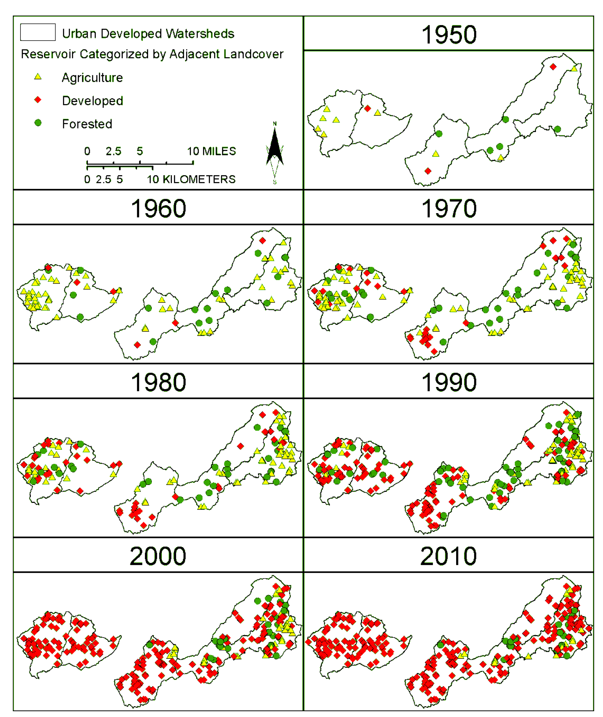
The dominant land cover adjacent to reservoirs changed over time and varied by region (
Figure 3). In watersheds that are classified as either dominantly rural developed or urban developed based on 2001 NLCD, aerial photography showed the regions were largely agricultural as of 1950 and the land cover associated with most reservoirs remained agricultural until as recently as 1980. For example, within the urban developed watersheds, there were 62 agricultural, 52 developed, and 30 forested reservoirs in 1980 (
Figure 3 and
Figure 4). In contrast, in watersheds that are dominantly agricultural or forested based on the 2001 NLCD, these respective land cover types have remained the dominant land cover associated with most reservoirs since 1960.
Figure 4.
Map of reservoirs (classified by adjacent land cover) in urban developed watersheds, 1950–2010.
Figure 4.
Map of reservoirs (classified by adjacent land cover) in urban developed watersheds, 1950–2010.
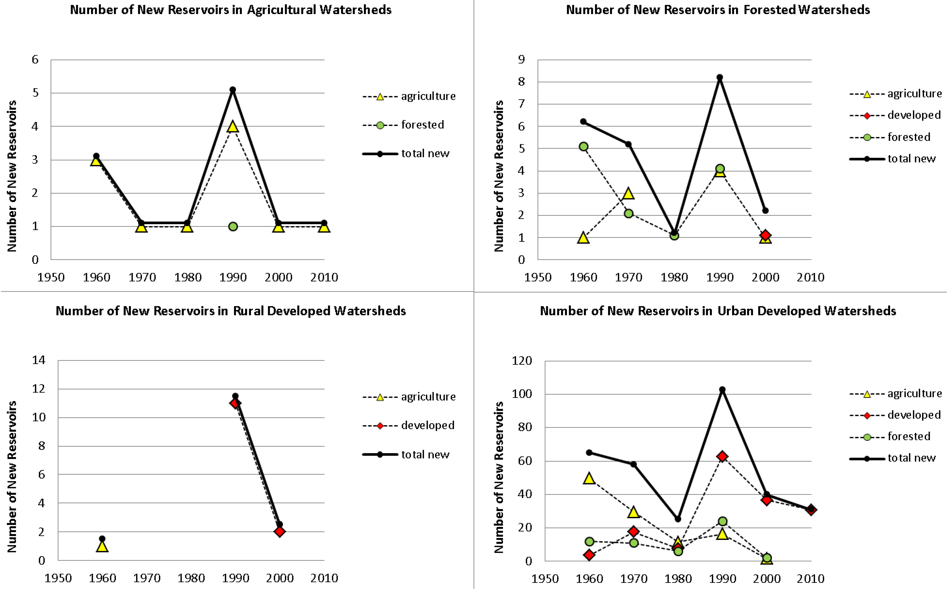
Despite the general trend in reservoir accumulation, some reservoirs were lost due to abandonment or demolition during the study period. Therefore, rather than only examining reservoir totals, it is helpful to separately consider the temporal trends in new reservoir construction during the study period (
Figure 5). Across all study watersheds, reservoir construction was primarily agricultural from 1950 to 1980. This period was followed by the most marked increase in new reservoir creation in all watersheds, occurring between 1980 and 1990. Finally, the boom in reservoir construction was followed by a sharp decline in reservoir construction during the 1990s and 2000s.
Change in inundated or “wetted” reservoir surface area is difficult to compare over time because of fluctuating water levels related to shifting weather and the varying seasonal conditions associated with inconsistent imagery acquisition dates. However, consideration of the full reservoir boundary (inundated area and dry reservoir bed) provides insight into the relative size of constructions and their impact in terms of habitat change and potential contributions to evaporation.
Surface area trends show that the average size of individual reservoirs steadily declined over time (
Table 3). Reservoirs constructed prior to 1960 were substantially larger in size with an average surface area of 0.045 km
2 while the average surface area consistently remained less than 0.012 km
2 in all subsequent years. However, in terms of total inundated area, the increase in the number of reservoirs meant that a higher percentage of the study area became inundated with water between 1950 and 2010. While 0.16% of the study area was covered by reservoirs in 1950, 0.95% was covered by reservoirs in 2010.
Figure 5.
Number of new small reservoirs classified by adjacent land cover for agricultural, forested, rural developed, and urban developed watersheds, 1950–2010. The highest peak in new reservoir construction occurred between 1980 and 1990 across all watershed categories.
Figure 5.
Number of new small reservoirs classified by adjacent land cover for agricultural, forested, rural developed, and urban developed watersheds, 1950–2010. The highest peak in new reservoir construction occurred between 1980 and 1990 across all watershed categories.
Table 3.
Classified by adjacent land cover, average reservoir surface area (km2) across all 20 study watersheds.
Table 3.
Classified by adjacent land cover, average reservoir surface area (km2) across all 20 study watersheds.
| Year | 1950 | 1960 | 1970 | 1980 | 1990 | 2000 | 2010 |
|---|
| agriculture | 0.80 | 0.82 | 0.75 | 0.87 | 0.56 | 0.62 | 0.64 |
| developed | 11.12 | 5.87 | 1.94 | 1.19 | 1.06 | 0.99 | 0.94 |
| forested | 1.69 | 2.42 | 1.67 | 1.59 | 1.22 | 1.16 | 0.88 |
| all reservoirs | 4.54 | 3.04 | 1.45 | 1.22 | 0.95 | 0.92 | 0.82 |
In terms of surface area and reservoir type, while agricultural reservoirs were dominant in number across nearly all watersheds from 1950 to 1980 (
Figure 3), their average surface area was smaller than the average surface area of the relatively fewer developed and forested reservoirs (
Table 3).
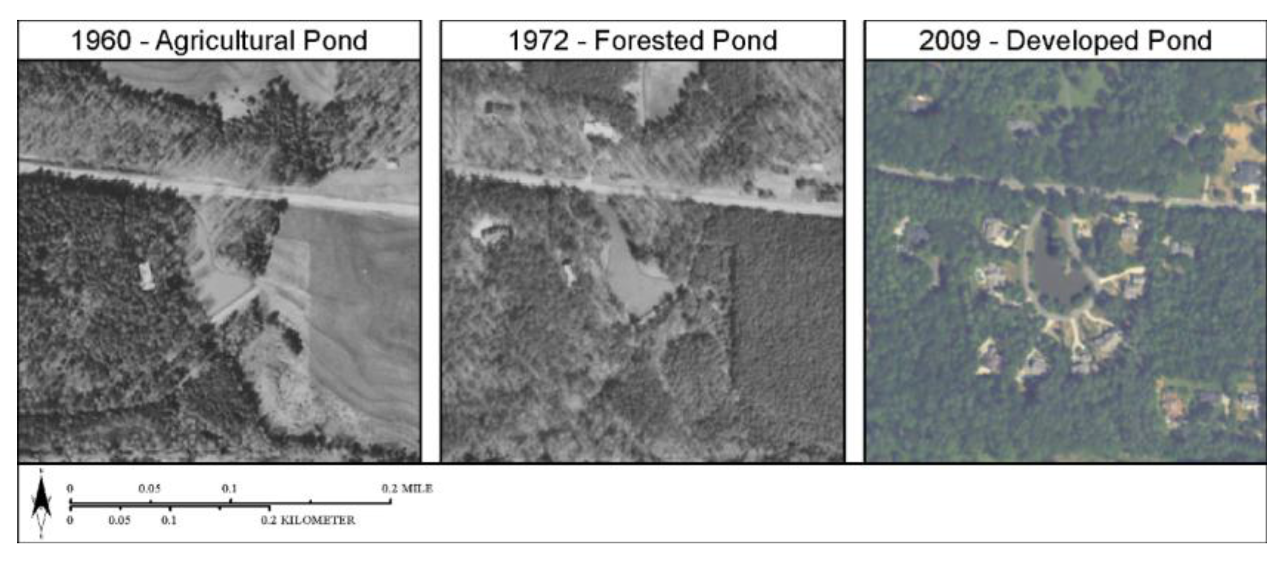
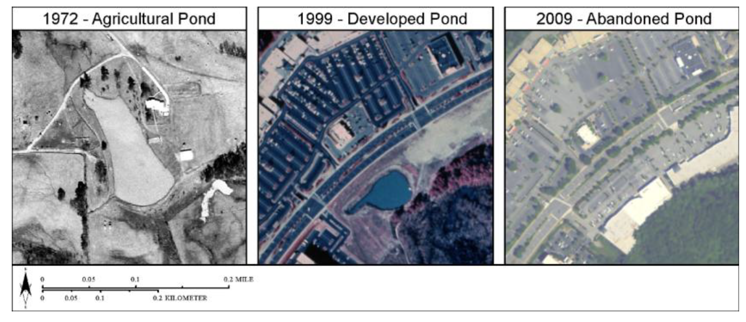
From 1950 to 2010, land cover change occurred throughout all study watersheds but was most apparent in the rural developed and urban developed watersheds. The rural developed watersheds transitioned from agriculture to rural development during the 1980s. In contrast, the urban developed watersheds transitioned from agriculture to forest and finally to urban developed land cover. This trend follows patterns recognized by other landscape change analyses [
67,
68,
69,
70]. For example, a reservoir in Fulton County, Georgia, was initially created as a farm reservoir in the 1950s (
Figure 6). By 1972 farming had stopped and the reservoir was left to become surrounded by reforestation. By 2009, the same reservoir became an amenity feature for urban development as large homes were constructed nearby and within view of the reservoir.
Figure 6.
Example of land cover modification adjacent to a small reservoir. Adjacent land cover changes from agricultural, to forested, to developed.
Figure 6.
Example of land cover modification adjacent to a small reservoir. Adjacent land cover changes from agricultural, to forested, to developed.
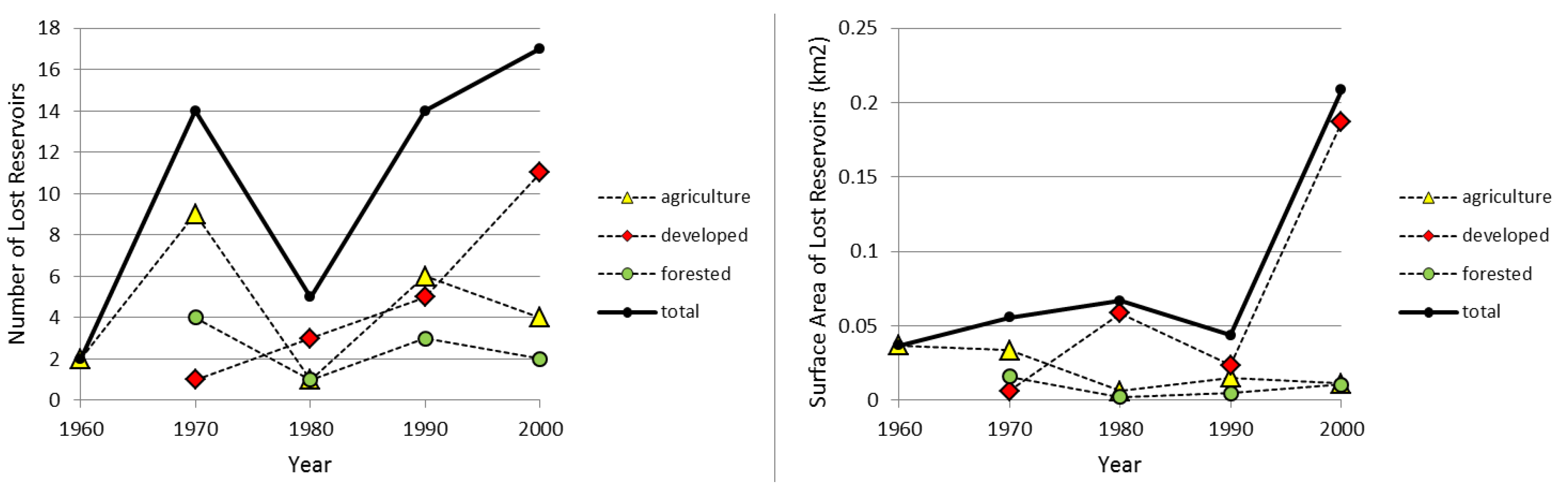
Figure 7.
Number and acreage of small reservoirs abandoned during prior decade in urban developed watersheds from 1960 to 2000 (only one reservoir was abandoned in other study watersheds). Reservoirs are classified by adjacent land cover immediately prior to abandonment.
Figure 7.
Number and acreage of small reservoirs abandoned during prior decade in urban developed watersheds from 1960 to 2000 (only one reservoir was abandoned in other study watersheds). Reservoirs are classified by adjacent land cover immediately prior to abandonment.
Figure 8.
Example of small reservoir and surrounding land cover change from agricultural to developed to abandoned (in this example, paved over).
Figure 8.
Example of small reservoir and surrounding land cover change from agricultural to developed to abandoned (in this example, paved over).
Abandoned reservoirs were another important trend over the 60-year study period. In total, out of the 382 reservoirs identified for all years and watersheds, 53 were abandoned by 2010. One reservoir was abandoned in a forested watershed while all other abandoned reservoirs were located in the urban developed watersheds. In the urban developed watersheds, agricultural reservoir abandonment peaked in the 1970s with a secondary surge in the 1990s, while abandoned reservoirs surrounded by developed land steadily increased through time (
Figure 7). Twenty of the abandoned reservoirs were originally constructed as agricultural reservoirs during the 1950s and 1960s. Many of these farm reservoirs were later modified into developed reservoirs, and then subsequently drained, overgrown, or filled-in and paved over by 2010 (
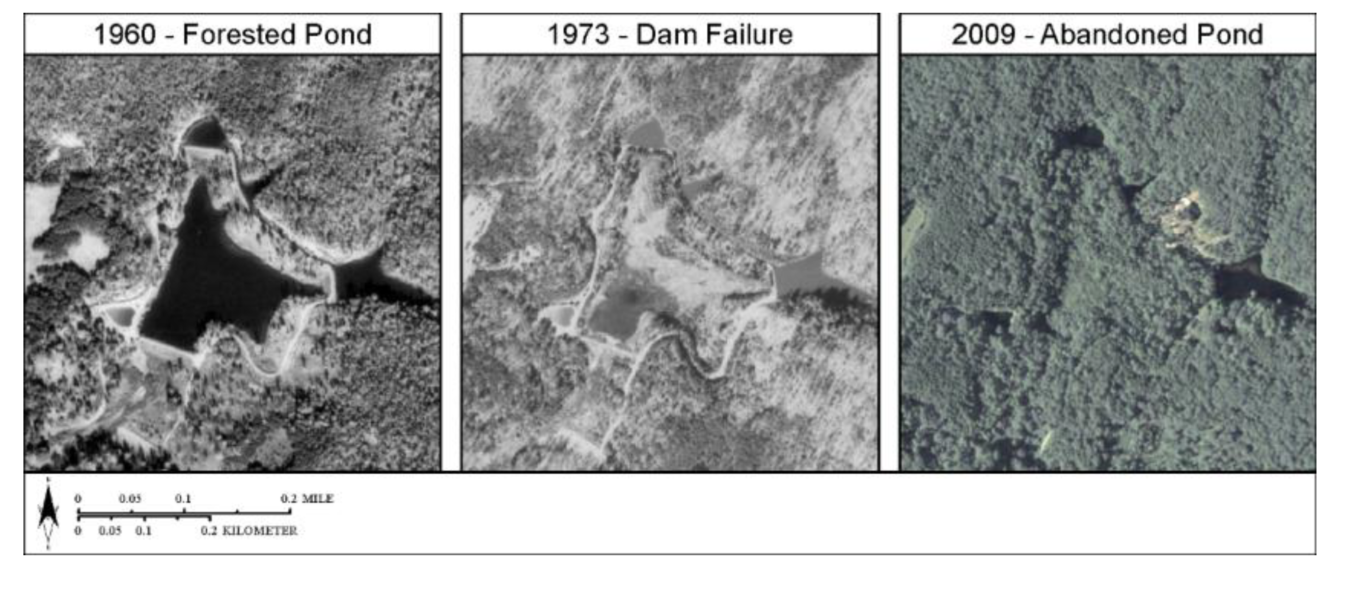
Figure 8). At least one of the abandoned forested reservoirs shows signs of dam failure and reforestation (
Figure 9).
Figure 9.
Example of small reservoir failure and abandonment.
Figure 9.
Example of small reservoir failure and abandonment.
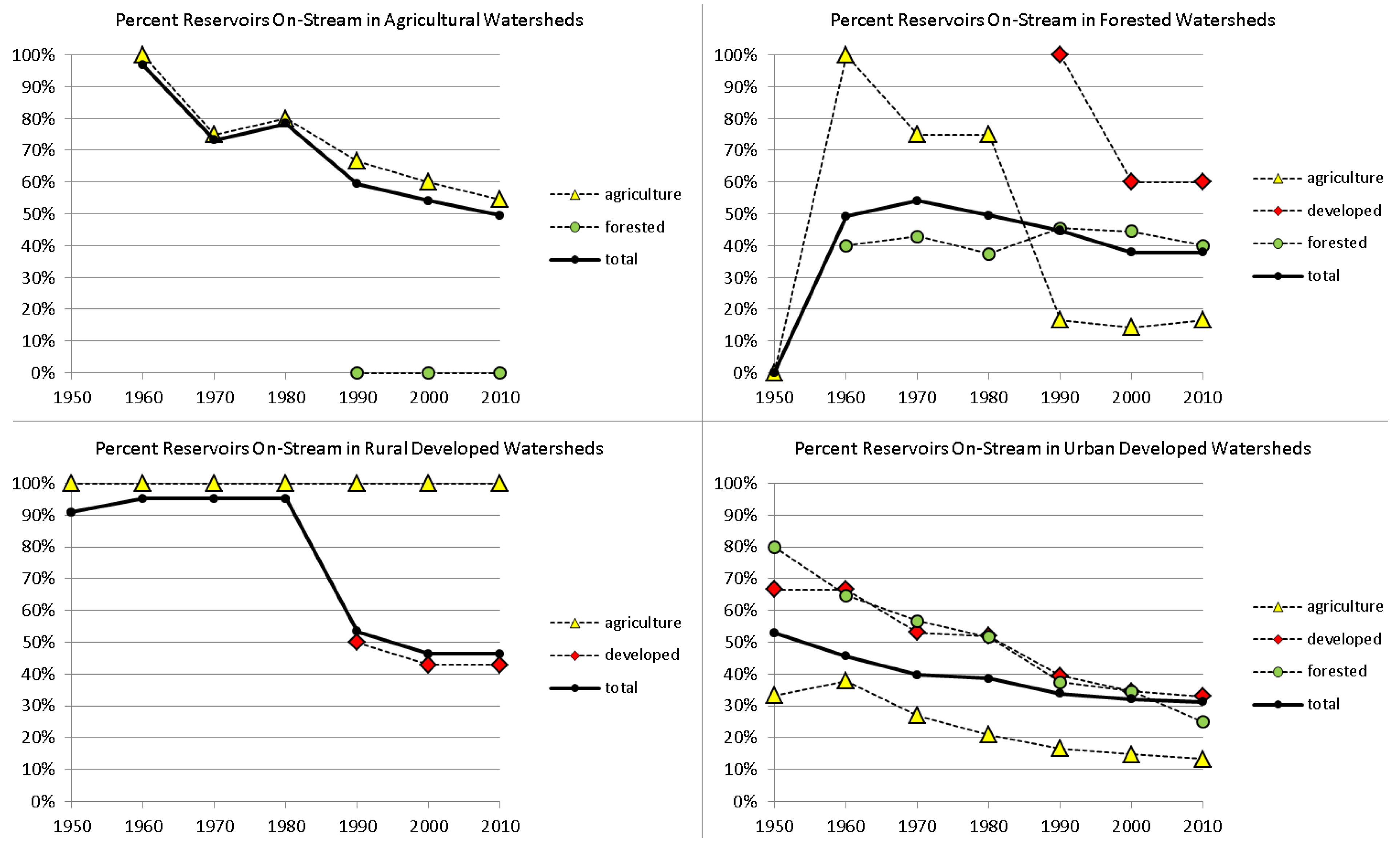
Figure 10.
Percent reservoirs (classified by adjacent land cover) located on-stream and causing stream fragmentation (based on intersection with the National Hydrography Dataset Flowline) for agricultural, forested, rural developed, and urban developed watersheds, 1950–2010. Reservoirs created after 1980 are less likely to intersect streams than previously constructed reservoirs.
Using the USGS NHD Flowline shapefile, reservoir polygons were intersected with linear stream data to examine the impact of reservoir creation on stream fragmentation over time. Over the 60-year study period, reservoir-stream intersections increased from 10 fragmentations in 1950 to 109 fragmentations in 2010. The increase in stream fragmentations was also present within each separate watershed category during the period from 1950 to 2010; fragmentations increased from zero to six for agricultural watersheds, from zero to eight for forested watersheds, from one to seven for rural watersheds, and from nine to 88 for urban watersheds. Considering all watersheds cumulatively, between 33% and 53% of reservoirs were located on-stream during the entire study period. In addition, analysis of the percent of on-stream reservoirs provides insight into the relative impact of reservoirs over time. Reservoirs created before 1980 were more likely to intersect streams than subsequently constructed reservoirs (
Figure 10).
5. Discussion
Throughout the study area, the number of reservoirs and the area inundated by water increased substantially during the 60-year study period (19 reservoirs covering 0.16% of the study area in 1950 to 329 reservoirs covering 0.95% of the study area by 2010). The nearly six-fold increase in reservoir surface area underscores the importance of pond construction in terms of land cover alteration in the Georgia Piedmont. The increase in inundated surface area has implications for an array of issues including water balance (e.g., evaporation), aquatic habitat availability, invasive species, and species migration patterns.
The timing of reservoir construction is also important as the majority of reservoirs across the study area were constructed within the last 30 years. The impact of small reservoirs constructed after 1980 on species distribution and genetic isolation has not yet been documented. In addition, the recent increase of reservoir construction indicates that even without maintenance, these features still have many years remaining before succumbing to sedimentation, dam failure, or re-forestation [
10].
Throughout the U.S., construction rates have followed different patterns for large
versus small reservoirs. Large reservoir creation peaked during the water engineering boom of the 1950s and 1960s [
71,
72]. After the 1970s, large reservoir construction tapered off as many ideal sites had already been utilized [
73]. Awareness of the high financial and ecological costs of dam construction also shifted water policy away from large reservoir construction during that time [
74]. In the upper and middle Chattahoochee River basins, small reservoir construction exhibited three distinct periods of reservoir creation: (1) prior to 1970 a steady number of forested and agricultural reservoirs were constructed; (2) the 1980s was the greatest period of developed reservoir creation; and (3) during the 1990s and 2000s there was a steep reduction in small reservoir construction.
These three periods of small reservoir creation (pre-1970, 1980s, and 1990–2010) reflect regional land cover trends and are correlated with different eras of government policies. The peak in agricultural reservoir construction prior to 1970 reflects the dominant agricultural land cover as much of the region was still used for cotton farming or had been abandoned and allowed to reforest [
66]. In addition, multiple Federal incentive programs promoted reservoir construction to encourage livestock agriculture and control sediment. Federal funds were provided for small reservoir creation through cost-sharing and fish-stocking programs [
2,
41]. During the 1980s, the boom in reservoir creation was likely spurred by new suburban growth surrounding the Atlanta metropolitan area [
58]. Urban reservoirs are commonly constructed to capture pollutants and excess sediment from construction sites and as stormwater run-off mitigation features [
43,
75]. In addition, these urban reservoirs are then treated as amenity features for housing developments or as recreational features for municipal parks. Finally, the decline in reservoir construction during the 1990s and 2000s is likely a result of expanding urbanization of much of the study area during this time [
58]. However, the lack of natural barriers around Atlanta [
58] indicates that urban/suburban growth and associated small reservoir construction will likely continue to expand into adjacent areas. More research is needed to determine whether high rates of reservoir construction were maintained in the suburban expansion beyond our study area.
Particularly within the urban developed watershed, the landscape transition from agricultural to forested to developed was caused by multiple factors including mid-20th century cropland abandonment followed by a transition from forested to developed land [
76]. Multiple factors contributed to the suburban expansion, including the increasing appeal of nonmetropolitan areas, decreasing household size, and decreasing density of settlement [
74]. Land cover change analyses within the metropolitan Atlanta region have documented rapid increases in high-density and low-density urban land cover and the loss of cropland and forests between 1973 and 1999 [
77]. The peak in small reservoir construction during suburban development underscores the importance of small reservoir research in newly industrializing areas and regions characterized by urban and suburban expansion. The impacts of reservoir construction may be particularly important in newly developing areas as hydrologic networks are commonly already degraded in urbanized watersheds [
43].
Despite the focus on developed reservoir construction within the study area, within other regions of the U.S. and globally, agricultural reservoir construction also remains prominent [
78]. Agricultural reservoir construction continues to be promoted as a vital part of water resources management to increase agricultural productivity and mitigate high stream flows, soil erosion, flooding, and nutrient influx to the Gulf of Mexico [
79]. In addition, farm reservoirs are promoted as a way to reduce agricultural impacts by increasing bird populations as part of a landscape mix containing both larger wetlands and small constructed ponds [
80].
Changes in land cover adjacent to reservoirs demonstrate their varied functions and shifting value over time. For example, modification of reservoirs from agricultural to recreational features shows that a single construction can serve multiple roles in the landscape and serve diverse purposes depending on societal needs. However, the frequency of reservoir abandonment reveals that these structures often have short lifespans. Small reservoirs are prone to gradually in-fill with sediment, may dry-up due to leakage or dam failure, and may be prohibitively expensive for landowners to maintain [
9]. Pond abandonment peaked during the 1960s as a result of agricultural reservoir reforestation and during the 1990s as a result of draining or building-over developing sites. The shifting land cover pattern from agricultural to forested to developed is reflected in these reservoir trends [
74].
Small reservoirs also play a major role in terms of stream fragmentation. During the 60-year study period, across all 20 study area watersheds, 33%–53% of reservoirs were located on-stream, causing between 10 and 109 stream fragmentations at any given time. The number of stream fragmentations is noteworthy as on-stream and off-stream reservoirs have very different implications for hydrology and ecology. On-stream reservoirs fragment habitat by isolating species from upstream reaches of the stream network [
25]. On-stream reservoirs also contribute to aquatic habitat conversion by altering riverine streams to lake-like lacustrine environments. These reservoirs have more direct impacts in terms of modifying stream physico-chemical properties and causing geomorphic changes [
3,
70]. Disconnected ponds have different environmental implications. In the absence of transient connectivity caused by extreme flow events, disconnected ponds less directly alter stream water quality but nonetheless may strongly impact water quantity and flow regimes by detaining water and contributing to evaporative losses [
23].
Within the study area, the decreasing percent of reservoirs located on-stream after 1980 may be caused by the lack of available pond sites on-stream after that date. In addition, before suburban expansion, the area was less fragmented, giving landowners more options about where to site reservoirs for larger inflows [
58]. Finally, it must be noted that while the stream polyline shapefile used in the analysis (NHD Flowline) captures both perennial and ephemeral streams, the 1;24,000 scale of the database inadequately captures many small headwater streams [
62,
81]. Therefore, stream-reservoir intersections should be interpreted as a minimum number of instances where reservoirs are located on-stream.
Dam removal is often discussed as a restoration strategy to alleviate the negative impacts associated with on-stream reservoirs [
82,
83,
84,
85]. Removing a dam can have especially positive implications for riverine ecologic health [
40]. However, there are also problematic factors associated with dam removal such as downstream morphological and habitat alteration caused by influxes of mobilized (and often contaminated) sediment previously held back by the dam [
86]. In addition, the ability to remove dams is impeded in landscapes characterized by multiple private landowners [
81]. The cooperation or interest of individual landowners and other (potentially numerous) stakeholders who may have conflicting interests [
56,
57] makes dam removal planning at the watershed scale quite difficult.


