Modeling Properties of Influenza-Like Illness Peak Events with Crossing Theory

Abstract

The concept of “peak event” has been used extensively to characterize influenza epidemics. Current definitions, however, could not maximize the amount of pertinent information about the probabilities of peak events that could be extracted from the generally limited available records. This study proposes a new method of defining peak events and statistically characterizing their properties, including: annual event density, their timing, the magnitude over prescribed thresholds and duration. These properties of peak events are analyzed in five counties of Florida using records from the Influenza-Like Illness Surveillance Network (ILINet). Further, the identified properties of peak events are compared between counties to reveal the geographic variability of influenza peak activity. The results of this study illustrate the proposed methodology’s capacity to aid public health professionals in supporting influenza surveillance and implementing timely effective intervention strategies.

1. Introduction

Influenza, widely known as the flu, is a highly contagious and acute respiratory disease. For a typical season, influenza activity often peaks in one or more weeks when the observed number of cases is noticeably higher than other weeks. These peak weeks incorporate a high proportion of influenza cases during the entire epidemic and are referred to variously as “peak events” or “peak weeks”. The properties of influenza peak events, such as timing, magnitude and duration, offer critical implications in disease surveillance, dynamics and control policies [1,2]. For example, the potential magnitude of peak events provides crucial information about the scale of an outbreak and suggests the amount of health resources in response to the disease [3]. The frequency, timing and duration of peak events offer a statistical basis for health insurance companies and long-term public health planning [4], e.g., the risk of more than one such event in a year and the length of time that each may persist. Because of their significance in epidemiology and planning, the study of such events has received increasing attention in recent years [5,6,7].

Although the concept of peak events is widely used in influenza-related studies, their workable definition remains under-studied. The traditional definition of “peak event” is an annual maximum. Smith [8] defined the “peak event” as the week with the greatest number of weekly influenza cases during an influenza season. This widely used definition is straightforward; however, it has the potential to exclude other events with epidemiological importance that may have occurred in a year and to include the annual maximum in the sample, which really does not constitute an event of epidemiological importance. Valuable information concerning epidemics, such as spatial variations, dynamics and periodicity, cannot be derived from the generally short historic records by this definition. Sakai et al. [9] slightly modified this approach by identifying the annual maximum of the smoothed data. They incorporated information from weeks before and after the peak event by smoothing data with a five-week unweighted moving average of weekly reported cases. The risk of this approach is that it obscures the important characteristics of the greatest number of influenza-like illness (ILI) cases in a week and may induce apparent periodic behavior in what could, in reality, be a random process. More importantly, these existing definitions of peak events offer little consideration to spatial heterogeneity, for instance, differences in demographics, and thus, the peak events alone are not comparable between geographic areas.

The limitations of existing definitions call for a more sophisticated approach employing spatially differentiated data that characterize weekly influenza activity and maximizing the pertinent information that may be extracted from the limited available records. As the first step in an on-going study that seeks to establish associations between ILI peak events and potential factors, this study aims to define ILI peak events and statistically characterize their properties: annual event density, their timing, magnitude over prescribed thresholds and duration.

2. Materials and Methods

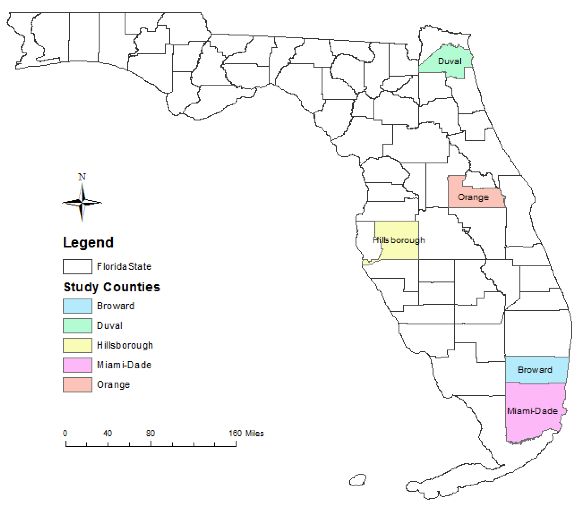
2.1. Study Area and Data

Florida experienced an average of 2900 estimated deaths per year from influenza over the past decade [10]. In 2004, for example, influenza and pneumonia together were the eighth leading cause of death reported by the Florida Department of Health (DOH) [11]. The Florida DOH estimates that an influenza pandemic could infect up to 10 million [12]. Several factors encourage the rapid transmission of influenza in the state: its developed tourism industry, high inter- and intra-national immigration and high proportion of aged population and their living styles. Despite its sub-tropical location and peninsular nature, much of Florida experiences periods of relatively low temperatures and low humidity in winter. Nearly one third of the population, including a large proportion of immigrants, resides in urban or suburban areas of three southeastern counties. Several interstates and 13 international airports, including Orlando and Miami, bring in tens of thousands of tourists each year (38 million used air travel in 2000 alone).

Data employed in this study are obtained from the Influenza-Like Illness Surveillance Network (ILINet), which conducts surveillance of weekly ILI outpatient cases [13]. The ILI case is defined as any combination of fever (≥38 °C) and cough or sore throat, which may embed influenza along with other conditions, such as colds and pneumonia. ILI activity collected through outpatient illness surveillance provides important epidemiologic information for monitoring influenza activity and supports influenza surveillance [14,15]. Weekly reports from ILINet are available dating back to 2001 in some counties; however, most counties did not have the necessary continuity of reporting at the earliest stages. As representatives of environmental, demographic and social conditions in Florida, five counties are selected for extensive study (Figure 1): the lengthy (2001–2012) historic data from dominantly urban Broward (Fort Laderdale), Duval (Jacksonville) and Miami-Dade (Miami) counties, as well as shorter (2006–2012) records for Orange (Orlando) and Hillborough (Tampa) counties.

Figure 1. The five selected counties in Florida.

Figure 1. The five selected counties in Florida.

2.2. Methodology

Crossing theory states that the number of crossings of a threshold by a Gaussian process become Poisson distributed the further the threshold lies from the mean of the process [16,17]. Results have also been extended to non-Gaussian processes [18] and can be applied to estimate the characteristics of ILI events. The magnitudes of events over the threshold and their durations can be approximated by an exponential-like distribution, such as the generalized Pareto distribution (GPD) [19,20], which can represent such data exhibiting both greater and lesser skew than the exponential itself. In combination with the Poisson assumption, it implies that the annual maximum or “peak week” [8] follows a generalized extreme value (GEV) distribution [19], the properties of which can be estimated from this approach, if desired. In general, the criteria for adopting a specific distribution are; the goodness-of-fit, a strong theoretical basis and the relative ease of computation and interpretation. Although few influenza-related studies have focused on the statistical properties of peak events, the proposed approach has been extensively used in studies modeling extremes in various fields, including floods, stock market returns and daily maximum temperatures [19,20,21].

The statistical properties of influenza events may all be defined by the prescription of a specific threshold. To facilitate spatial comparisons, this study defines the threshold in terms of common percentiles of historic weekly ILI cases (i.e., defined in the frequency domain); although for epidemiological or planning purposes, the threshold could be defined in the magnitude domain, in terms of the total number of ILI cases of particular interest. Results extracted above the 80th percentile level (0.20 probability of occurring in any week) are extrapolated to the more rarely experienced levels equivalent to the 90th (0.10 probability) and 95th percentiles (0.05 probability) and compared to the small available sample of historic events that exceed these higher levels. In this way, a larger proportion of the limited available historic records can be utilized to characterize properties of ILI events above levels commonly witnessed.

Definitions of events and the flu year are established first. Then, the variables of interest are identified: (1) annual event density (events per year); (2) the timing (t) of each event; (3) the magnitude of the peak event (τ = x − q₀) during an event when the observed number of weekly cases (x) surpasses the thresholds (q₀); and (4) the duration of events.

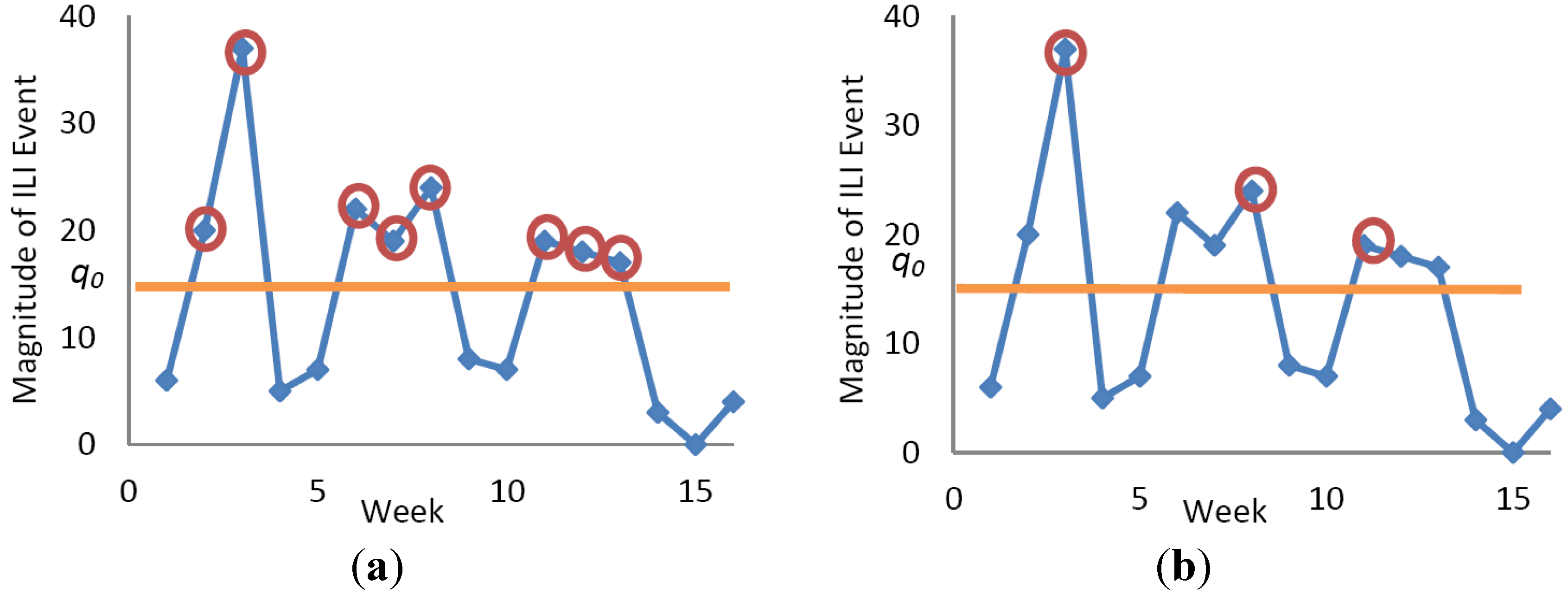
2.2.1. Definitions of Events

Although thresholds (q₀) are considered in terms of percentiles of historic weekly ILI cases throughout the study, two definitions of the magnitudes of events are investigated. The first includes all weeks with an absolute weekly ILI count greater than the prespecified threshold. In Figure 2a, for example, all the eight ILI observations greater than the defined threshold would be considered (one or more observations of the magnitude per event). The second definition considers only the week with the highest ILI count above the threshold within the period between successive up- and down-crossings of the threshold level (one observation of the magnitude per event)—a local maximum. In Figure 2b, only the three observations of local maxima would be considered. The properties of ILI peak events are examined above a commonly witnessed 80th percentile level, although this approach is applicable for any other reasonably high thresholds.

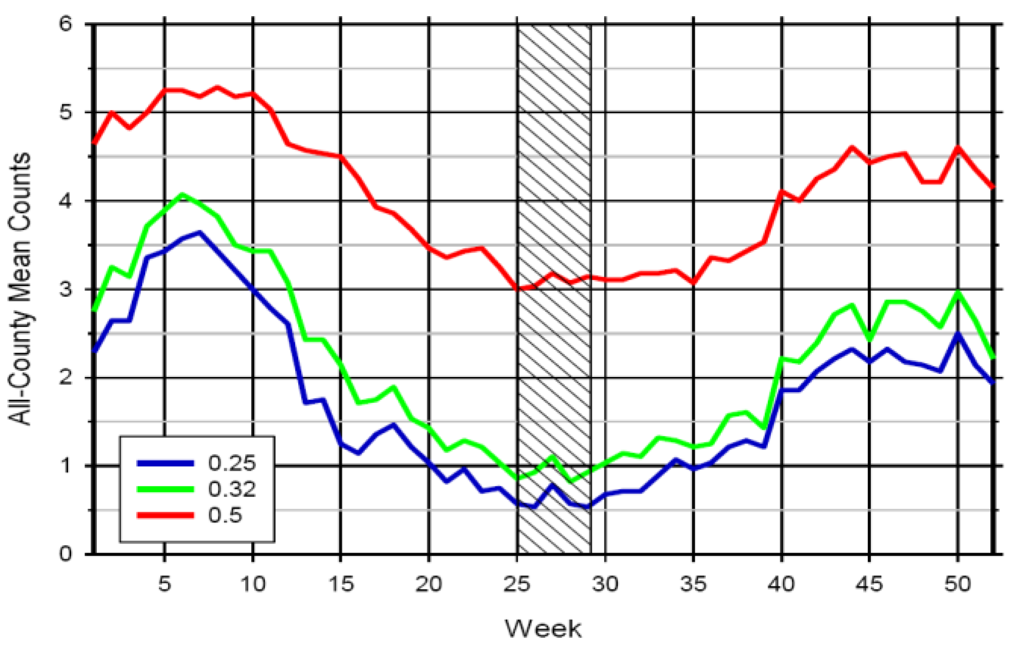
2.2.2. Definition of Flu Year

Since all ILI cases are likely to be recorded during the winter season, the use of a calendar year definition would arbitrarily bisect a flu season, producing a misleading aggregation of events from two halves of consecutive and distinct seasons. To determine when flu is least likely to occur in the historic record (an appropriate point to start and finish a “flu year”), the occurrence of ILI events throughout Florida is analyzed using the mean (µ) and defined fractions of the standard deviations (0.25σ, 0.32σ and 0.5σ) of all weekly ILI cases. In terms of the mean weekly occurrence in all counties in Florida (Figure 3), Week 29 (starting 15 July) is the week in which ILI cases are least likely by this measure and is thus defined as the beginning of the “flu year”, noted hereafter as “Week 1”.

Figure 2. Definitions of magnitudes above the threshold. (a) Definition 1. (b) Definition 2. The blue curve represents weekly influenza-like illness (ILI) cases; the red circle represents the selected peak; and the orange line represents the threshold (q₀).

Figure 2. Definitions of magnitudes above the threshold. (a) Definition 1. (b) Definition 2. The blue curve represents weekly influenza-like illness (ILI) cases; the red circle represents the selected peak; and the orange line represents the threshold (q₀).

Figure 3. The mean weekly occurrence of ILI events in all counties based on the defined standard deviations (0.25σ, 0.32σ and 0.5σ).

Figure 3. The mean weekly occurrence of ILI events in all counties based on the defined standard deviations (0.25σ, 0.32σ and 0.5σ).

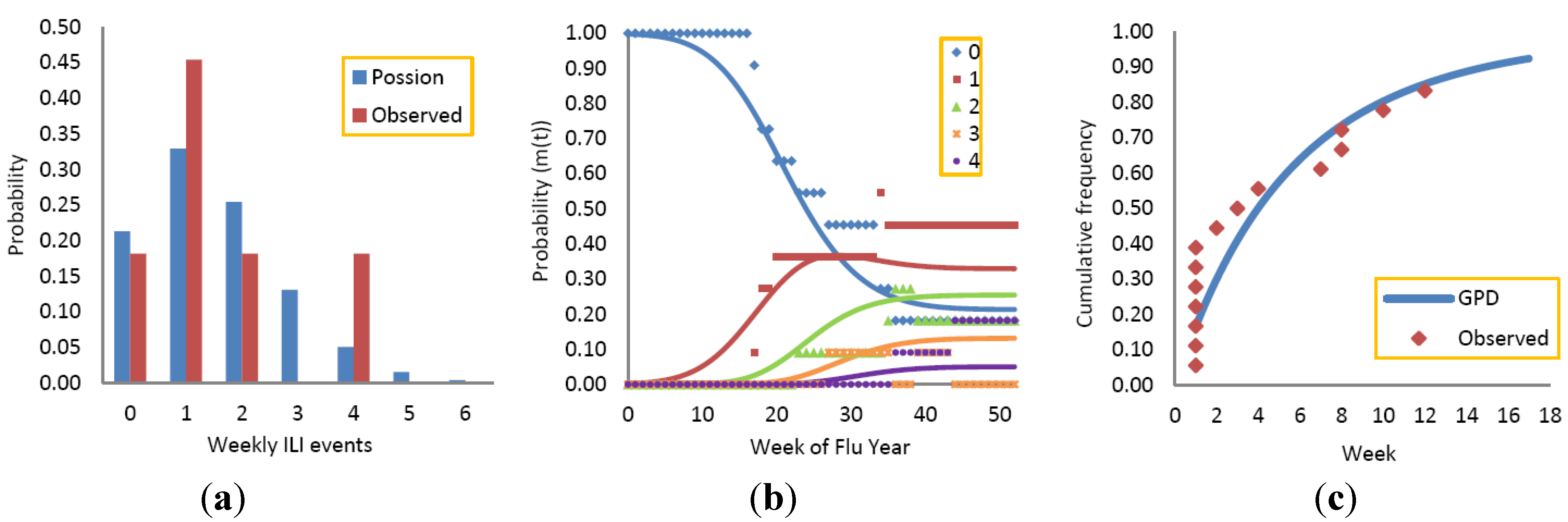
2.2.3. Annual Event Density

Annual event density is defined as the number of events per flu year. The probability mass function of the Poisson distribution is:

P(M) = e^−Λ × Λ^M / M!

(1)

where M is the number of events in a flu year and Λ is estimated using the method of moments as the mean number of events per flu year:

Λ = K / N

(2)

K is the total number of events in N flu years with complete yearly data in the historic records.

2.2.4. Timing of Events within a Flu Year

Due to the strong seasonal nature of ILI cases, the Poisson distribution is modified to exhibit a time-dependent rate of event occurrence, λ(t):

P(m(t) = n) = e^−λ(t) × λ(t)ⁿ / n!

(3)

where P(m(t) = n) is the probability of having experienced n events up to and including week t and λ(t) is the mean number of events expected up to that time. As influenza outbreaks generally occur in a particular season with some interannual variability, the timings of events are modeled by a Gaussian distribution and λ(t), estimated as,

λ(t) = G(t: μ, σ) × Λ

(4)

where G(t: μ, σ) is a Gaussian distribution fitted to the observed timing of ILI events, with μ being the mean week of occurrences and σ their standard deviation.

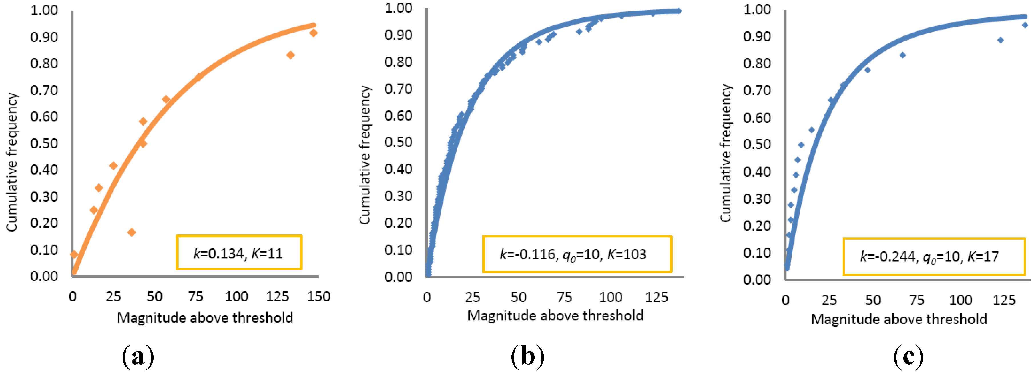
2.2.5. Event Magnitude

The distribution of event magnitudes is fit with a GPD [19,20]:

(5)

where X is the magnitude of the event over the predetermined threshold of interest. Completely characterized by a scale parameter, α, and a shape parameter, k, the GPD is a generalization of both the exponential (k = 0) and Pareto distributions (k < 0), which provides greater flexibility in matching the heavier (k < 0) and thinner (k > 0) upper tails of the distribution. The parameters are estimated via the method of moments from the sample mean, , and variance as Equations (6) and (7):

(6)

(7)

2.2.6. Event Duration

The duration of events is also represented by the GPD [20]:

(8)

where D is the duration of the event, representing total weeks related to a peak event. Similarly, α′ and k′ are scale and shape parameters, which are estimated via the method of moments by Equations (6) and (7), using appropriate means and variances.

2.2.7. Independence of Events

A period of two consecutive weeks in which the weekly ILI cases fall below the threshold level is employed as the criterion to separate independent peak events. Occasions when weekly cases dropped marginally below the threshold level only to exceed it again in the next week are probably the result of the same event. Parallel considerations in the definition of flood and heat wave events can be found in Rosbjerg et al. [19] and Keellings and Waylen [20]. “Events” failing to meet this independence criterion are combined and included in subsequent analysis as if they constitute a single event.

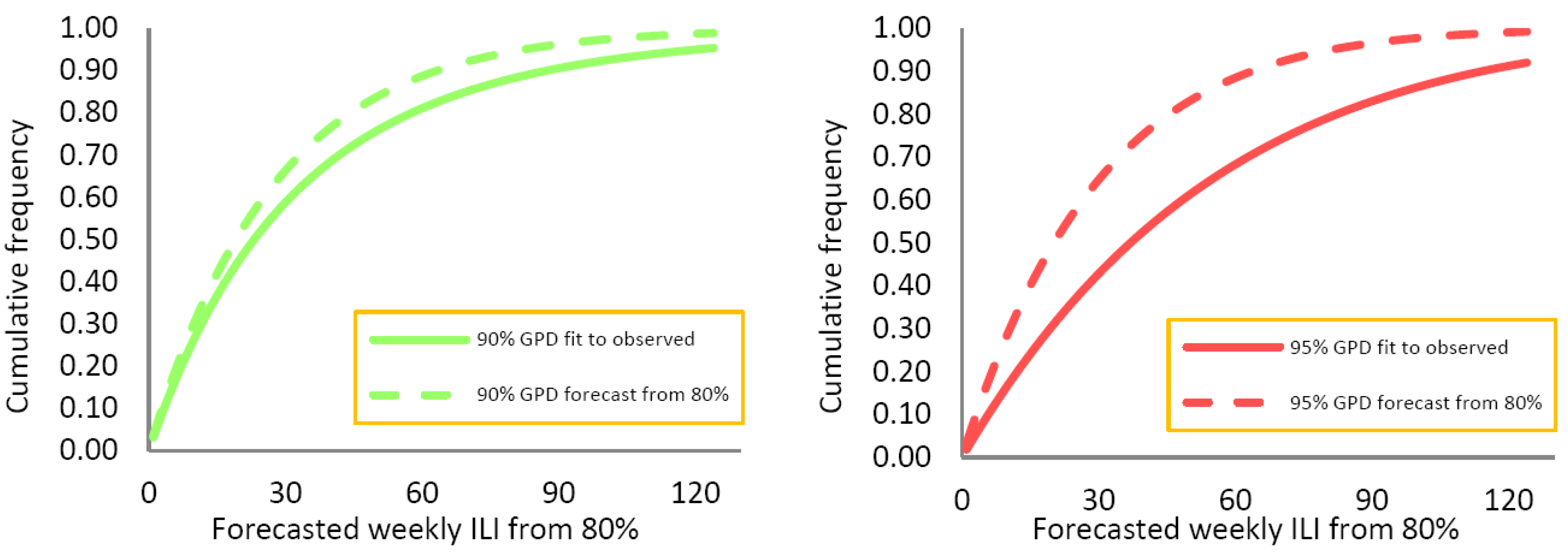
2.2.8. Extrapolation of Properties to Higher Thresholds

An ability to derive the stochastic properties of ILI events above higher, less commonly experienced levels, from the larger sample sizes available at the lower, less epidemiologically-important thresholds, would be useful. Any portion of a GPD is itself GPD-distributed; thus, the process of raising the threshold is effectively “cutting off” the lower end of GPD and leaving only that portion that rises above the new level. Estimation of the mean (μ₁) and variance (σ₁) of the remaining portion of the distribution yields revised estimates of α₁ and k₁ (Equations (6) and (7)). The proportion of events expected to exceed the higher threshold represented by the area under the original distribution of magnitudes, which lies beyond the new level, yields the parameter, Λ₁, of the Poisson distribution. The probability of the annual number of crossings above the corresponding threshold, or events, can then be estimated. Assuming that the timing and magnitudes of ILI events are independent, the distribution of the timing of censored events should remain unchanged.

3. Results

3.1. Annual Numbers of Events, Their Timings and Durations

The one-sample Kolmogorov–Smirnov test is applied to examine the goodness-of-fit of all models. All results show no significant differences between fitted and observed distributions at the 0.05 level of significance in any of the five study counties. The assumption of normality of the timing of peak events is reasonable graphically and statistically. Data from the longer-term record of Duval County are examined as an example.

Figure 4. Annual event density, timing and duration at the 80th percentile level in Duval County. (a) Annual event density. (b) Timing plots. The probabilities of zero, one, two, three and four events having occurred, in Duval County, up to any week during the flu year. (c) The duration of peak events. GPD, generalized Pareto distribution.

Figure 4. Annual event density, timing and duration at the 80th percentile level in Duval County. (a) Annual event density. (b) Timing plots. The probabilities of zero, one, two, three and four events having occurred, in Duval County, up to any week during the flu year. (c) The duration of peak events. GPD, generalized Pareto distribution.

Historic ILI events are most likely to occur during the late fall and early spring (Weeks 20 to 32 of the flu year), coincident with conducive meteorological conditions and the early weeks of the spring semester of school. The Poisson probability function is fitted to the numbers of events exceeding the 80th percentile level annually (Figure 4a), and the non-homogeneous Poisson function is applied in order to estimate probabilities of experiencing zero, one, two, three and four events up to any week of the flu year (Figure 4b). This reproduces well the observed patterns of occurrence during late fall and early spring. Taking Week 26 in the flu year (the second week of January) as an example, the probability of having experienced no peak events up to that time (m(t) = 0) is 0.43; the probability of exactly one peak event is 0.36, etc. The probability of an ILI event occurring in a particular week, t, can be computed as {[P(m(t − 1) = 0)] − [P(m(t) = 0)]}. The generalized Pareto distribution provides a reasonable approximation to the distribution of the likely durations of events at the 80th percentile level (Figure 4c).

3.2. Magnitudes of Events and Comparisons of Definitions

Figure 5 illustrates the GPD’s ability to model the observed cumulative distribution function (CDF) based on either of the two definitions of magnitudes. The location parameter, α, conveys information about the relative magnitude of the cases above the threshold in each county and could be standardized to some base, such as estimated total county population, while the values of k can be compared directly between counties. As expected, the sample sizes derived using Definition 1 (Figure 5b) are much larger than that using Definition 2 (Figure 5c). Negative values of the shape parameter, k, imply that, at this relatively low threshold, the upper tail is particularly “heavy” (larger outliers in the right-hand tail of the distribution) in comparison to the bulk of observations.

Figure 5. Cumulative distribution functions (CDFs) of observed magnitudes over the 80th percentile level based on three definitions in Duval County. (a) Traditional definition. (b) Definition 1. (c) Definition 2. Note: q₀ represents the threshold ILI cases for each level, and K represents the total number of peak events in all flu years.

Figure 5. Cumulative distribution functions (CDFs) of observed magnitudes over the 80th percentile level based on three definitions in Duval County. (a) Traditional definition. (b) Definition 1. (c) Definition 2. Note: q₀ represents the threshold ILI cases for each level, and K represents the total number of peak events in all flu years.

3.3. Extrapolation of Weekly ILI Cases to Higher Levels

The parameters of the above distributions are simply estimated by the application of moment estimators to data extracted at the 80th percentile level. The proposed methodology has the capacity to yield distributions of events exceeding higher, more rarely experienced levels (for example, here, the 90th and 95th percentile levels) from the larger sample sizes of observations gathered at the lower truncation level (the 80th percentile level) (Figure 6).

Figure 6. Forecasted magnitudes over the 90th and 95th percentile levels from the 80th percentile level in Duval County.

Figure 6. Forecasted magnitudes over the 90th and 95th percentile levels from the 80th percentile level in Duval County.

When the critical threshold for Duval county is raised from 10 cases (the 80th percentile level) to 23 (the 90th percentile level), the observed mean annual number of events drops from 1.55 per flu year to 0.91 (Table 1). The GPD fitted to the local maxima of events indicates that 58.5% of the original 17 events should exceed the increased threshold, yielding an anticipated mean annual number of events of 0.90. If the critical threshold is raised to 41 cases (the 95th percentile level), and the observed mean annual number of events drops to 0.45, while 30.8% of the original 17 events (0.48 events per year) are anticipated to exceed this increased threshold. The use of higher thresholds levels leads to the exclusion of the bulk of the lower magnitude events, reducing the “heaviness” of the tail of the surviving events and increasing the values of k.

4. Discussions

Grounded in theory, this approach has the ability to describe important statistical properties of such events and provides the necessary degree of flexibility in the definition of ILI events, while permitting spatial comparisons and the handling of various planning scenarios. Once the suitable probability distributions are identified, the probability of the occurrence of ILI events and their properties can be obtained for further specified purposes.

4.1. Comparisons of Definitions

The traditional definition of peak events only captures an annual maximum (magnitude) in each flu year, but discards other important properties of annual event density and duration and runs the risk of including “peak” events of no epidemiological significance. The proposed approach possesses the benefit of only including ILI events that meet the level of practical interest, while incorporating a potentially larger sample size from the short records currently available. The traditional “peak week” definition applied to Duval County yields 11 observations, while the application of the 80th percentile threshold increases the available sample size upon which risk can be estimated to 103 using Definition 1 and 17 for Definition 2 (Figure 5). Once estimated, the parameters of the GPD provide the basis for the estimation of properties above successively higher, more rarely observed, levels of ILI incidence. The threshold of interest can be expressed either in terms of acceptable risk (frequency domain) for spatial comparisons, or case numbers (magnitude domain) for planning purposes.

Table 1. Summary of observed and expected parameters of ILI peak events upon raising the thresholds to the 90th and 95th percentile levels (Definition 2).

Name	Years of Record	80th Percentile				90th Percentile					95th Percentile
		Timings		Mean Duration d	Mean Number of Events Λ	Timings		Mean Duration d	Mean Number of Events Λ (O/E)		Timings		Mean Duration d	Mean Number of Events Λ (O/E)
		Mean μ	Standard Deviation σ			Mean μ	Standard Deviation σ				Mean μ	Standard Deviation σ
Broward	11	24.91	10.76	5.36	2.00	24.33	10.40	3.39	1.64	1.45 (72.3%)	21.75	12.24	2.33	1.09	0.83 (41.5%)
Duval	11	25.06	8.33	6.35	1.55	28.50	6.88	5.30	0.91	0.90 (58.5%)	25.60	7.83	6.20	0.45	0.48 (30.8%)
Miami-Dade	11	26.21	12.34	6.05	1.73	29.82	10.07	5.27	1.00	0.88 (50.8%)	26.33	9.46	4.83	0.55	0.56 (32.2%)
Hillsborough	6	22.63	10.57	7.63	1.33	23.56	12.65	3.22	1.50	1.02 (76.7%)	28.50	8.81	5.25	0.67	0.59 (49.8%)
Orange	6	29.90	11.79	6.50	1.67	31.40	14.79	6.00	0.83	0.85 (50.9%)	23.00	10.44	4.67	0.50	0.45 (26.7%)

Table 1. Summary of observed and expected parameters of ILI peak events upon raising the thresholds to the 90th and 95th percentile levels (Definition 2).

Name	Years of Record	80th Percentile				90th Percentile					95th Percentile
		Timings		Mean Duration d	Mean Number of Events Λ	Timings		Mean Duration d	Mean Number of Events Λ (O/E)		Timings		Mean Duration d	Mean Number of Events Λ (O/E)
		Mean μ	Standard Deviation σ			Mean μ	Standard Deviation σ				Mean μ	Standard Deviation σ
Broward	11	24.91	10.76	5.36	2.00	24.33	10.40	3.39	1.64	1.45 (72.3%)	21.75	12.24	2.33	1.09	0.83 (41.5%)
Duval	11	25.06	8.33	6.35	1.55	28.50	6.88	5.30	0.91	0.90 (58.5%)	25.60	7.83	6.20	0.45	0.48 (30.8%)
Miami-Dade	11	26.21	12.34	6.05	1.73	29.82	10.07	5.27	1.00	0.88 (50.8%)	26.33	9.46	4.83	0.55	0.56 (32.2%)
Hillsborough	6	22.63	10.57	7.63	1.33	23.56	12.65	3.22	1.50	1.02 (76.7%)	28.50	8.81	5.25	0.67	0.59 (49.8%)
Orange	6	29.90	11.79	6.50	1.67	31.40	14.79	6.00	0.83	0.85 (50.9%)	23.00	10.44	4.67	0.50	0.45 (26.7%)

Table 2. Observed and expected parameters of magnitudes upon raising the thresholds to the 90th and 95th percentile levels (Definition 1). Note: q₀, the threshold; α, the scale parameter of GPD; k, the shape parameter of GPD; K, the total number of peak events in all flu years.

Name	Years of Record	80th Percentile				90th Percentile							95th Percentile
		q0	α	k	K	q0	α (O/E)		k (O/E)		K (O/E)		q0	α (O/E)		k (O/E)		K (O/E)
Broward	11	2	4.27	−0.30	93	4	5.36	5.83	−0.29	−0.20	54	60	8	6.85	7.19	−0.29	−0.19	25	41
Duval	11	10	22.52	−012	103	23	34.33	25.84	0.06	0.02	51	59	41	44.32	27.50	0.27	0.07	27	29
Miami-Dade	11	18	13.76	−0.16	102	27	15.55	16.75	−0.15	−0.05	53	55	34	26.55	17.94	0.06	−0.03	27	35
Hillsborough	6	24	20.09	−0.10	56	35	30.67	22.93	0.08	0.00	28	33	53	37.85	24.78	0.22	0.04	13	15
Orange	6	69	73.93	0.34	59	114	73.36	51.86	0.64	0.42	29	30	155	49.45	31.25	0.68	0.40	14	14

Table 2. Observed and expected parameters of magnitudes upon raising the thresholds to the 90th and 95th percentile levels (Definition 1). Note: q₀, the threshold; α, the scale parameter of GPD; k, the shape parameter of GPD; K, the total number of peak events in all flu years.

Name	Years of Record	80th Percentile				90th Percentile							95th Percentile
		q0	α	k	K	q0	α (O/E)		k (O/E)		K (O/E)		q0	α (O/E)		k (O/E)		K (O/E)
Broward	11	2	4.27	−0.30	93	4	5.36	5.83	−0.29	−0.20	54	60	8	6.85	7.19	−0.29	−0.19	25	41
Duval	11	10	22.52	−012	103	23	34.33	25.84	0.06	0.02	51	59	41	44.32	27.50	0.27	0.07	27	29
Miami-Dade	11	18	13.76	−0.16	102	27	15.55	16.75	−0.15	−0.05	53	55	34	26.55	17.94	0.06	−0.03	27	35
Hillsborough	6	24	20.09	−0.10	56	35	30.67	22.93	0.08	0.00	28	33	53	37.85	24.78	0.22	0.04	13	15
Orange	6	69	73.93	0.34	59	114	73.36	51.86	0.64	0.42	29	30	155	49.45	31.25	0.68	0.40	14	14

Table 3. Observed and expected parameters of magnitudes upon raising the thresholds to the 90th and 95th percentile levels (Definition 2). Note: q₀, the threshold; α, the scale parameter of GPD; k, the shape parameter of GPD; K, the total number of peak events in all flu years.

Name	Years of Record	80th Percentile				90th Percentile							95th Percentile
		q0	α	k	K	q0	α (O/E)		k (O/E)		K (O/E)		q0	α (O/E)		k (O/E)		K (O/E)
Broward	11	2	5.82	−0.35	22	4	5.75	7.85	−0.37	−0.23	18	16	8	5.67	9.50	−0.40	−0.21	12	9
Duval	11	10	22.69	−0.24	17	23	31.58	27.59	−0.16	0.00	10	10	41	55.13	29.82	0.09	0.07	5	5
Miami-Dade	11	18	12.16	−0.26	19	27	14.76	16.42	−0.23	−0.08	11	10	34	21.99	18.25	−0.13	−0.05	6	6
Hillsborough	6	24	41.54	−0.00	8	35	22.88	41.43	0.05	0.16	9	6	53	46.93	39.60	0.10	0.19	4	4
Orange	6	69	68.15	0.07	10	114	195.14	40.64	1.74	0.25	5	5	155	1921.63	19.54	34.37	0.09	3	3

Table 3. Observed and expected parameters of magnitudes upon raising the thresholds to the 90th and 95th percentile levels (Definition 2). Note: q₀, the threshold; α, the scale parameter of GPD; k, the shape parameter of GPD; K, the total number of peak events in all flu years.

Name	Years of Record	80th Percentile				90th Percentile							95th Percentile
		q0	α	k	K	q0	α (O/E)		k (O/E)		K (O/E)		q0	α (O/E)		k (O/E)		K (O/E)
Broward	11	2	5.82	−0.35	22	4	5.75	7.85	−0.37	−0.23	18	16	8	5.67	9.50	−0.40	−0.21	12	9
Duval	11	10	22.69	−0.24	17	23	31.58	27.59	−0.16	0.00	10	10	41	55.13	29.82	0.09	0.07	5	5
Miami-Dade	11	18	12.16	−0.26	19	27	14.76	16.42	−0.23	−0.08	11	10	34	21.99	18.25	−0.13	−0.05	6	6
Hillsborough	6	24	41.54	−0.00	8	35	22.88	41.43	0.05	0.16	9	6	53	46.93	39.60	0.10	0.19	4	4
Orange	6	69	68.15	0.07	10	114	195.14	40.64	1.74	0.25	5	5	155	1921.63	19.54	34.37	0.09	3	3

Although Definition 1 of magnitudes yields a larger sample size, their obvious serial auto-correlation results in less reliable estimates of the proportion of the observations surviving censoring to higher threshold levels; a task which is performed much better using magnitudes derived from Definition 2. Table 2 and Table 3 display the values of observed and predicted parameters describing the distribution of magnitudes under both definitions above increased truncation levels.

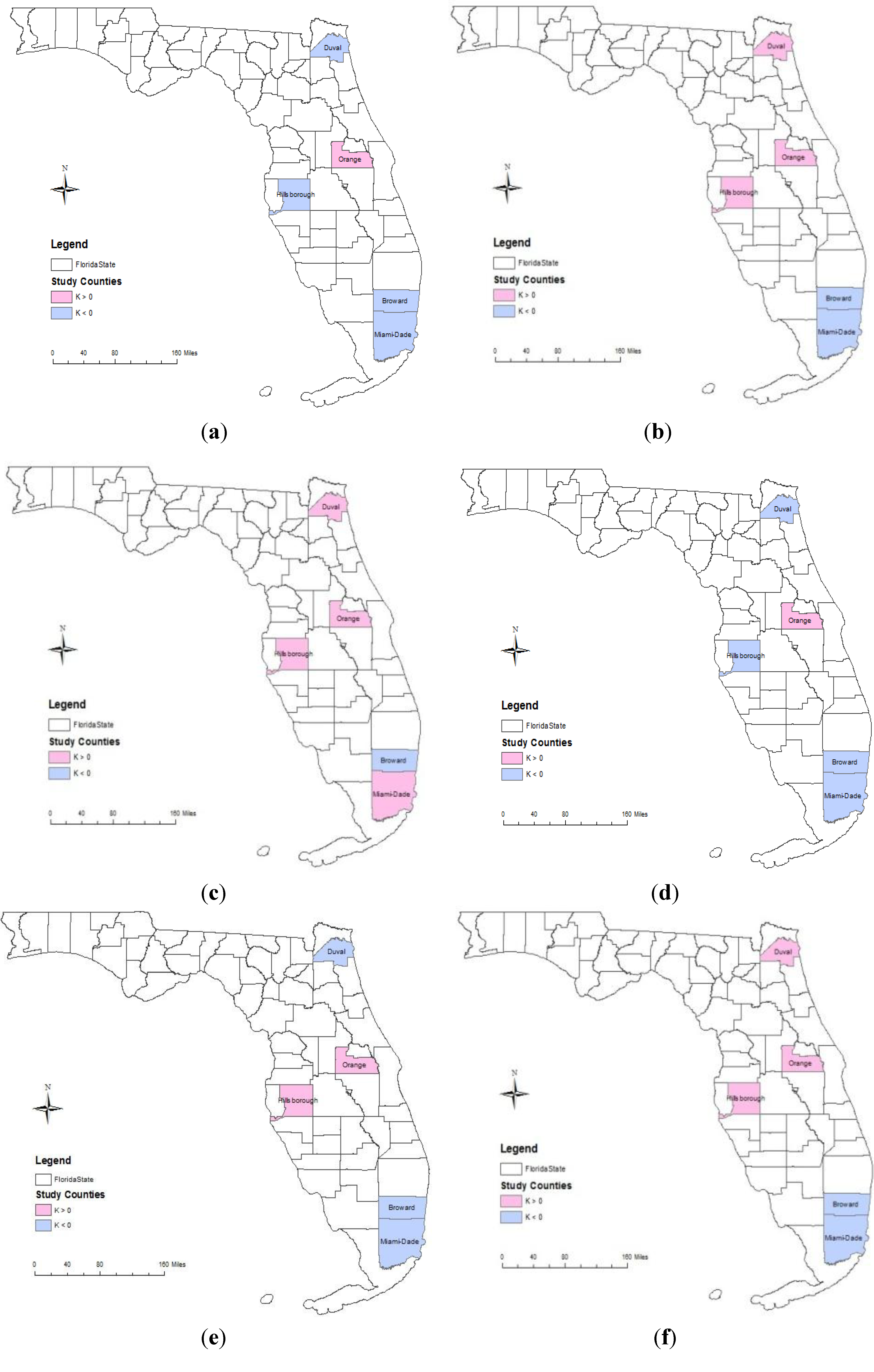
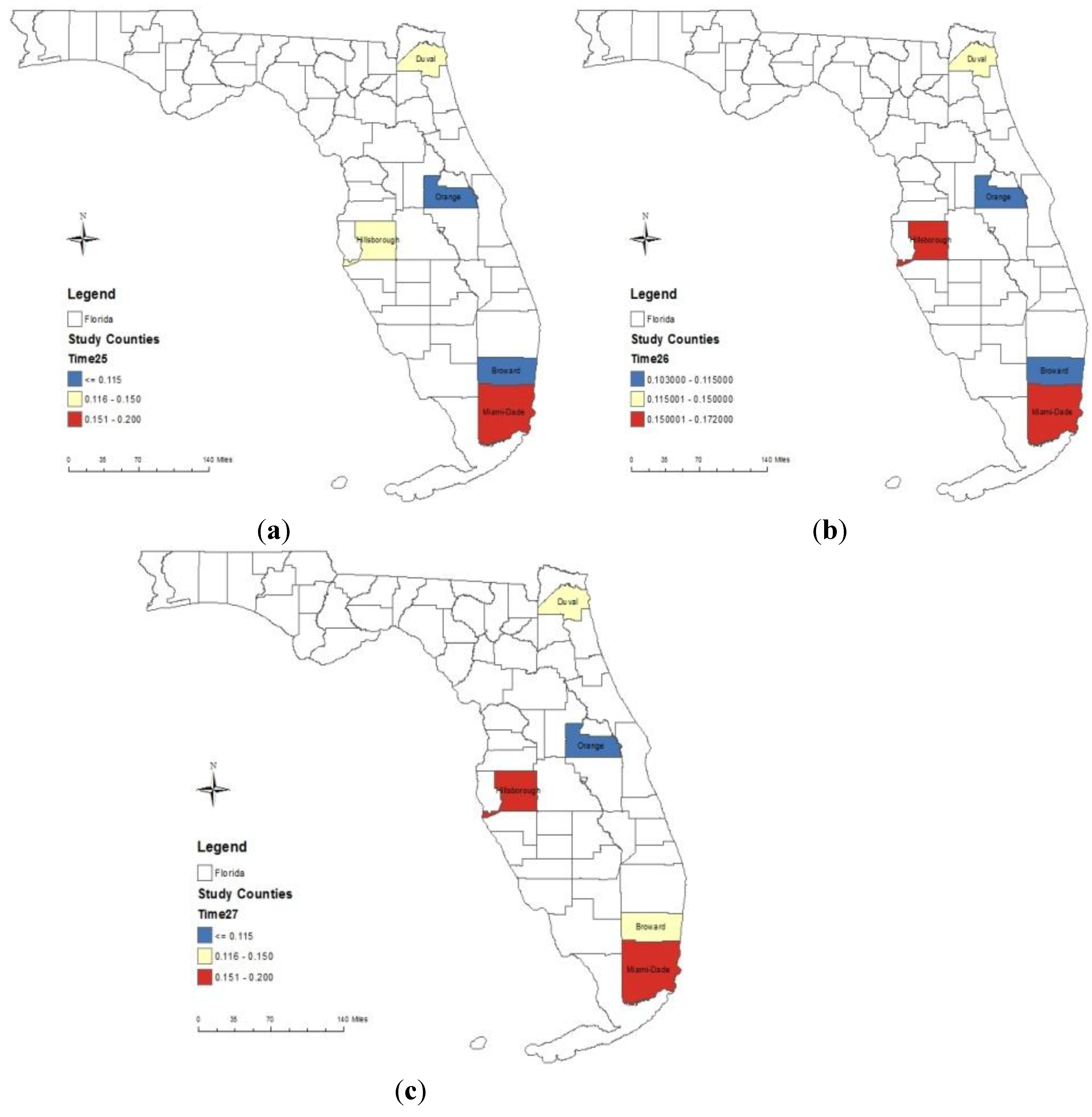
4.2. Geographic Variability and Potential Impacts

This study provides flexible models that render probabilistic estimates of the variables associated with ILI events that can be adapted to various conditions. The robust statistical methodology may be implemented at any location, no matter the base (e.g., population) and critical thresholds established. Geographic variability in the parameters indicates differences in the potential influences on the occurrence of ILI peak events. For example, the observed spatial pattern of the shape parameter, k, at the 80th, 90th and 95th percentile levels in Figure 7 suggests that at higher thresholds, more counties exhibit positive values, no matter the definition. Since k is, in the theory, independent of threshold and stable with respect to shifts in the threshold [22], it can be compared directly across spatially differentiated locations. Negative values of k indicate large outliers in the right-hand tail of the distribution relative to the bulk of the observations. The values of k become less negative at higher thresholds, because the comparative magnitudes of the outliers decrease as thresholds increase by progressive censoring. This is particularly noticeable when using Definition 1. It is likely to be over-interpreting due to the limited data, especially the small number of observations at a higher threshold. With increasing data availability in the future, a longer time period and a larger sample size can help to better represent these properties of ILI events.

Figure 7. The observed spatial distributions of the parameter, k, values at three thresholds based on two definitions. (a) Definition 1, threshold 80%-k. (b) Definition 1, threshold 90%-k. (c) Definition 1, threshold 95%-k. (d) Definition 2, threshold 80%-k. (e) Definition 2, threshold 90%-k. (f) Definition 2, threshold 95%-k.

Figure 7. The observed spatial distributions of the parameter, k, values at three thresholds based on two definitions. (a) Definition 1, threshold 80%-k. (b) Definition 1, threshold 90%-k. (c) Definition 1, threshold 95%-k. (d) Definition 2, threshold 80%-k. (e) Definition 2, threshold 90%-k. (f) Definition 2, threshold 95%-k.

As a highly contagious and acute respiratory disease, the occurrence and properties of ILI peak events may be influenced by environmental (weather, etc.), demographic and social (urban, rural, transportation, etc.) factors. This approach identifies the average week of occurrence as late fall to early spring (Weeks 22 to 30, starting 10 December to 6 February with fairly large standard deviations of eight to 12 weeks). These observations are supported physically by studies that influenza outbreaks are sensitive to the weekly or bi-weekly average temperatures and humidity [5,23], particularly low temperature (optimum: 8 °C) and relative humidity [23,24,25]. Mean temperatures during the coldest month in Florida across the counties examined range from 10 °C to 16 °C, suggesting that weather conditions may have impacts on spatial patterns of peak events. However, no clear spatial pattern related to latitude and winter temperatures emerges. As the critical level of ILI cases of interest rises, the mean week of timing for events increases (later in the year) in almost all counties, except Broward, implying that peak events with greater weekly ILI cases tend to occur during late winter and early spring. In addition to weather conditions, each county possesses features that encourage influenza transmission: high population density, high proportions of their populations in sensitive age groups, international airports and ready access to major interstates, all of which have potentially profound effects on the occurrence of ILI events [26,27,28,29]. Similarly comparative use of public transport and immunization behavior may cause differences in the course of epidemics and modify their space-time spread [30,31]. Orange County, for example, exhibits relatively high values of the threshold (q₀) and total numbers of peak events (K) compared to the other four counties. This might be explained by its special characteristics of being located in the center of the state with comparatively low temperature and relative humidity with respect to the two southern counties (Miami-Dade and Broward). The major city in Orange County, Orlando, receives tens of thousands of tourists annually, especially during holidays in the late fall and winter, increasing the possibility of influenza transmission, for example compared to the northern county (Duval). To better understand the spatial patterns of the derived properties of events, the impacts of the above factors deserve to be further examined.

4.3. Application

The spatio-temporal visualizations of these statistical properties have the potential to deliver information in an efficient manner and assist decision-making within public health, such as the early warning of influenza peak activity, determining where and when to intervene, increasing the accessibility of health facilities, etc. For example, Figure 8 visualizes the spatial and temporal patterns of the timing of peak events, which represents the probability of having two ILI peak events up to Week 25, Week 26 and Week 27. These weeks are the first three weeks in January. The increasing probability of having two peak events in Week 26 and Week 27 may be due to the possible impacts of cold weather in January and the new semester of school on ILI activity. These visualizations can be expanded to the entirety of Florida in the future.

Figure 8. Application of timing in 18 selected counties in Florida. (a) Probability of experiencing two events up to Week 25. (b) Probability of experiencing two events up to Week 26. (c) Probability of experiencing two events up to Week 27.

Figure 8. Application of timing in 18 selected counties in Florida. (a) Probability of experiencing two events up to Week 25. (b) Probability of experiencing two events up to Week 26. (c) Probability of experiencing two events up to Week 27.

5. Conclusions

This study innovatively applies an established method in hydrology and climatology to the field of epidemiology to describe the statistical properties of periods during which weekly ILI cases exceed critical thresholds. The new definition of events of interest beyond “peak events” considers only, and all, outbreaks of epidemiological interest and permits the estimation of the parameters of the distributions. The strong theoretical basis in crossing theory allows for the calculation of the properties of ILI events above various thresholds of interests. Another advantage of this approach is that it can be applied to spatially differentiated data to determine and compare risks associated with peak events, not defined by a common number of cases, but by a common frequency of outbreak regardless of the base population of the area (e.g., a weekly count that is only experienced in 20%, or 5%, of all the weeks of historic records in a county).

The methodology has the added flexibility of permitting the extrapolation of ILI event properties, especially the number of events and the magnitude, to other critical thresholds that vary in space and that are influenced by environmental, demographic and social factors. In the meantime, the potentially limited information contained in the standard ILI “peak event” (annual maximum) definition hinders public health professionals in efficiently implementing timing intervention strategies, such as vaccination and quarantine, thus leading to unnecessary socio-economic costs. This study can aid public health officials in supporting influenza surveillance and intervention by including the properties of the variables, annual event density, timing, magnitude and duration. The development and testing of these flexible models is the first step in an on-going study that seeks to establish associations between the statistical properties of ILI events and potential environmental factors. These associations can then be combined with vaccination and human mobility to give predictions of influenza transmission and to determine optimal periods to implement influenza vaccination programs among priority regions. Importantly, the models in this study could be easily extended to other infectious diseases in a further modification.

References

1. Fleming, D.M.; Zambon, M.; Bartelds, A.I.M.; de Jong, J.C. The duration and magnitude of influenza epidemics: A study of surveillance data from sentinel general practices in England, Wales and the Netherlands. Eur. J. Epidemiol. 1999, 15, 467–473. [Google Scholar] [CrossRef]
2. Bock, D.; Andersson, E.; Frisén, M. Statistical surveillance of epidemics: Peak detection of influenza in Sweden. Biom. J. 2008, 50, 71–85. [Google Scholar] [CrossRef]
3. Cooper, D.L.; Verlander, N.Q.; Elliot, A.J.; Joseph, C.A.; Smith, G.E. Can syndromic thresholds provide early warning of national influenza outbreaks? J. Public Health 2009, 31, 17–25. [Google Scholar]
4. Cowling, B.J.; Wong, I.O.; Ho, L.M.; Riley, S.; Leung, G.M. Methods for monitoring influenza surveillance data. Int. J. Epidemiol. 2006, 35, 1314–1321. [Google Scholar]
5. Charland, K.M.L.; Buckeridge, D.L.; Sturtevant, J.L.; Melton, F.; Brownstein, J.S. Does climate predict the timing of peak influenza activity in the United States? Adv. Dis. Surveill. 2008, 5, 169. [Google Scholar]
6. Greene, S.K.; Ionides, E.L.; Wilson, M.L. Patterns of influenza-associated mortality among US elderly by geographic region and virus subtype, 1968–1998. Am. J. Epidemiol. 2006, 163, 313–326. [Google Scholar]
7. Paget, J.; Marquet, R.; Meijer, A.; van Der Velden, K. Influenza activity in Europe during eight seasons (1999–2007): An evaluation of the indicators used to measure activity and an assessment of the timing, length and course of peak activity (spread) across Europe. BMC Infect. Dis. 2007, 7. [Google Scholar] [CrossRef]
8. Smith, L.P. Numerical forecasting of epidemics of influenza in Great Britain and Northern Ireland. Rev. Epidemiol. Sante Publique 1982, 30, 413–422. [Google Scholar]
9. Sakai, T.; Suzuki, H.; Sasaki, A.; Saito, R.; Tanabe, N.; Taniguchi, K. Geographic and temporal trends in influenza like illness, Japan, 1992–1999. Emerg. Infect. Dis. 2004, 10, 1822–1826. [Google Scholar] [CrossRef]
10. CDC WONDER Online Database. Underlying Cause of Death 1999–2009. Available online: http://wonder.cdc.gov/ucd-icd10.html (accessed on 11 November 2012).
11. Florida Department of Health. Available online: http://www.doh.state.fl.us/disease_ctrl/epi/htopics/flu/FSPISN/influenza_sentinels.html (accessed on 18 November 2012).
12. Florida Department of Health. Available online: http://www.doh.state.fl.us/disease_ctrl/epi/htopics/flu/panflu.htm (accessed on 15 November 2012).
13. Florida Department of Health. Available online: http://www.doh.state.fl.us/floridaflu/FSPISN/influenza_sentinels.html (accessed on 19 November 2012).
14. Centers for Disease Control and Prevention. Available online: http://www.cdc.gov/flu/weekly/overview.htm (accessed on 10 January 2013).
15. Cooley, P.; Ganapathi, L.; Ghneim, G.; Holmberg, S.; Wheaton, W.; Hollingsworth, C.R. Using influenza-like illness data to reconstruct an influenza outbreak. Math. Comput. Model. 2008, 48, 929–939. [Google Scholar] [CrossRef]
16. Cramer, H.; Leadbetter, M.R. Stationary and Related Stochastic Processes; Wiley: New York, NY, USA, 1967. [Google Scholar]
17. Rice, S.O. Mathematical analysis of random noise. Bell Syst. Tech. J. 1945, 24, 46–156. [Google Scholar] [CrossRef]
18. Desmond, A.F.; Guy, B.T. Crossing theory for Non-Gaussian processes with an application to hydrology. Water Resour. Res. 1991, 279, 2791–2797. [Google Scholar] [CrossRef]
19. Rosbjerg, D.; Madsen, H.; Rasmussen, P.F. Prediction in partial duration series with generalized pareto-distributed exceedances. Wat. Resour. Res. 1992, 28, 3001–3010. [Google Scholar] [CrossRef]
20. Keellings, D.; Waylen, P.R. The stochastic properties of high daily maximum temperatures applying crossing theory to modeling high-temperature event variables. Theor. Appl. Climatol. 2012, 108, 579–590. [Google Scholar] [CrossRef]
21. Straetmans, S.T.M.; Verschoor, W.F.C.; Wolff, C.C.P. Extreme US stock market fluctuations in the wake of 9/11. J. Appl. Econom. 2008, 23, 17–42. [Google Scholar]
22. Beisel, C.J.; Rokyta, D.R.; Wichman, H.A.; Joyce, P. Testing the extreme value domain of attraction for distributions of beneficial fitness effects. Genetics 2007, 176, 2441–2449. [Google Scholar] [CrossRef]
23. Lowen, A.C.; Mubareka, S.; Steel, J.; Palese, P. Influenza virus transmission is dependent on relative humidity and temperature. PLoS Pathog. 2007, 3, e151. [Google Scholar] [CrossRef]
24. Shaman, J.; Kohn, M. Absolute humidity modulates influenza survival, transmission, and seasonality. Proc. Natl. Acad. Sci. USA 2009, 106, 3243–3248. [Google Scholar] [CrossRef]
25. Tsuchihashi, Y.; Yorifuji, T.; Takao, S.; Suzuki, E.; Mori, S.; Doi, H.; Tsuda, T. Environmental factors and seasonal influenza onset in Okayama city, Japan: Case-crossover study. Acta Med. Okayama 2011, 65, 97–103. [Google Scholar]
26. Ertek, M.; Durmaz, R.; Guldemir, D.; Altas, A.B.; Albayrak, N.; Korukluoglu, G. Epidemiological, demographic, and molecular characteristics of laboratory-confirmed pandemic influenza A (H1N1) virus infection in Turkey. Jpn. J. Infect. Dis. 2010, 63, 239–245. [Google Scholar]
27. Olson, D.R.; Heffernan, R.T.; Paladini, M.; Konty, K.; Weiss, D.; Mostashari, F. Monitoring the impact of influenza by age: Emergency department fever and respiratory complaint surveillance in New York city. PLoS Med. 2007, 4, e247. [Google Scholar] [CrossRef]
28. Viboud, C.; Boëlle, P.Y.; Cauchemez, S.; Lavenu, A.; Valleron, A.J.; Flahault, A.; Carrat, F. Risk factors of influenza transmission in households. Br. J. Gen. Pract. 2004, 54, 684–689. [Google Scholar]
29. Rivas, A.L.; Chowell, G.; Schwager, S.J.; Fasina, F.O.; Hoogesteijn, A.L.; Smith, S.D.; Bisschop, S.P.; Anderson, K.L.; Hyman, J.M. Lessons from Nigeria: The role of roads in the geo-temporal progression of avian influenza (H5N1) virus. Epidemiol. Infect. 2009, 138, 192–198. [Google Scholar]
30. Lim, W.-Y.; Chen, C.-H.; Ma, Y.; Chen, M.-I.; Lee, V.-J.; Cook, A.-R.; Tan, L.W.; Flores Tabo, N., Jr.; Barr, I.; Cui, L.; et al. Risk factors for pandemic (H1N1) 2009 seroconversion among adults, Singapore, 2009. Emerg. Infect. Dis. 2011, 17, 1455–1462. [Google Scholar]
31. Yang, Y.; Sugimoto, J.D.; Halloran, M.E.; Basta, N.E.; Chao, D.L.; Matrajt, L.; Potter, G.; Kenah, E.; Longini, I.M., Jr. The transmissibility and control of pandemic influenza A (H1N1) virus. Science 2009, 326, 729–733. [Google Scholar] [CrossRef]