Spatial Representation of Coastal Risk: A Fuzzy Approach to Deal with Uncertainty


Abstract
:1. Introduction
2. Background
2.1. Spatial Representation of Coastal Erosion Risk

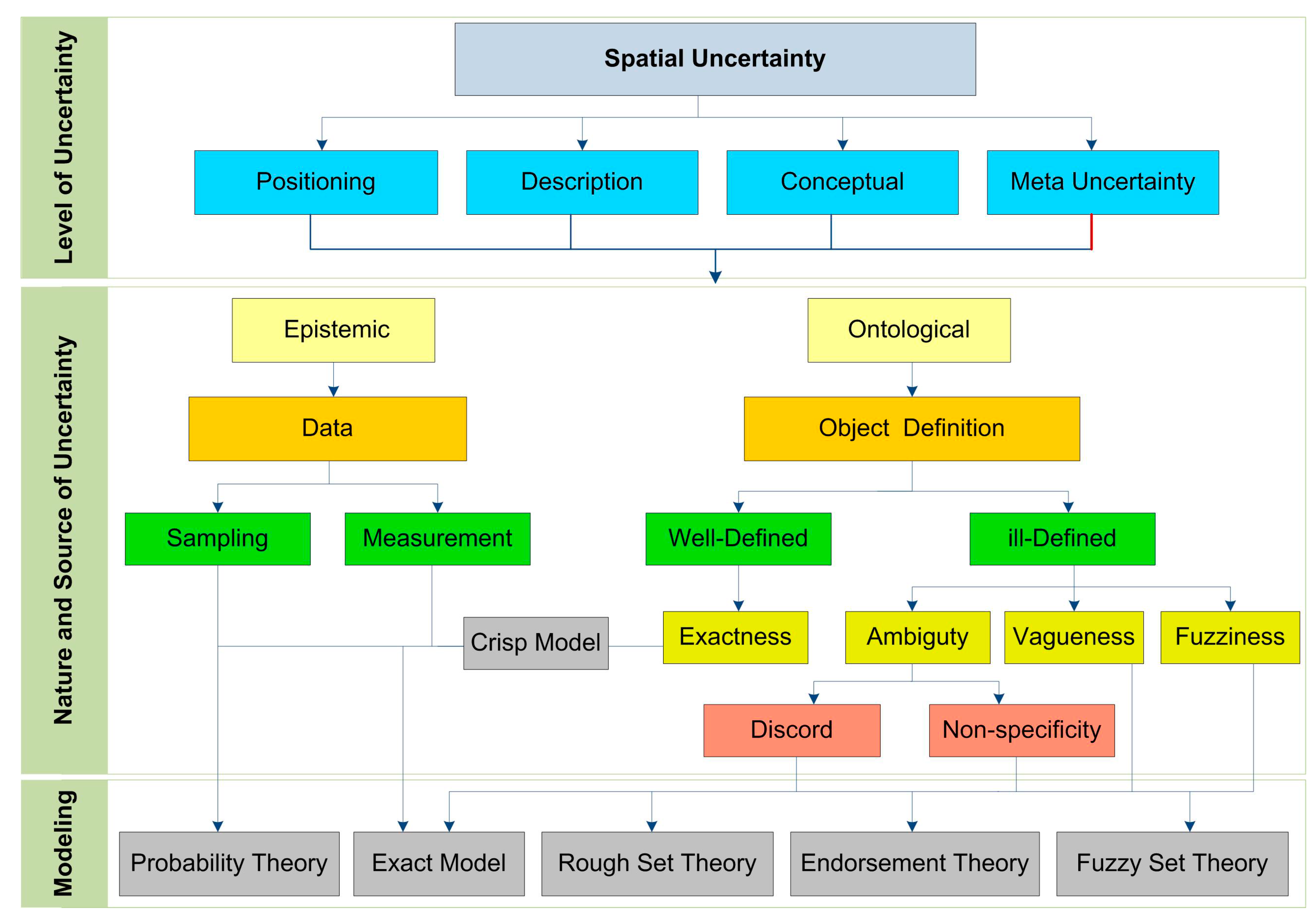
2.2. Uncertainty Characterization

3. Spatial Fuzzy Object
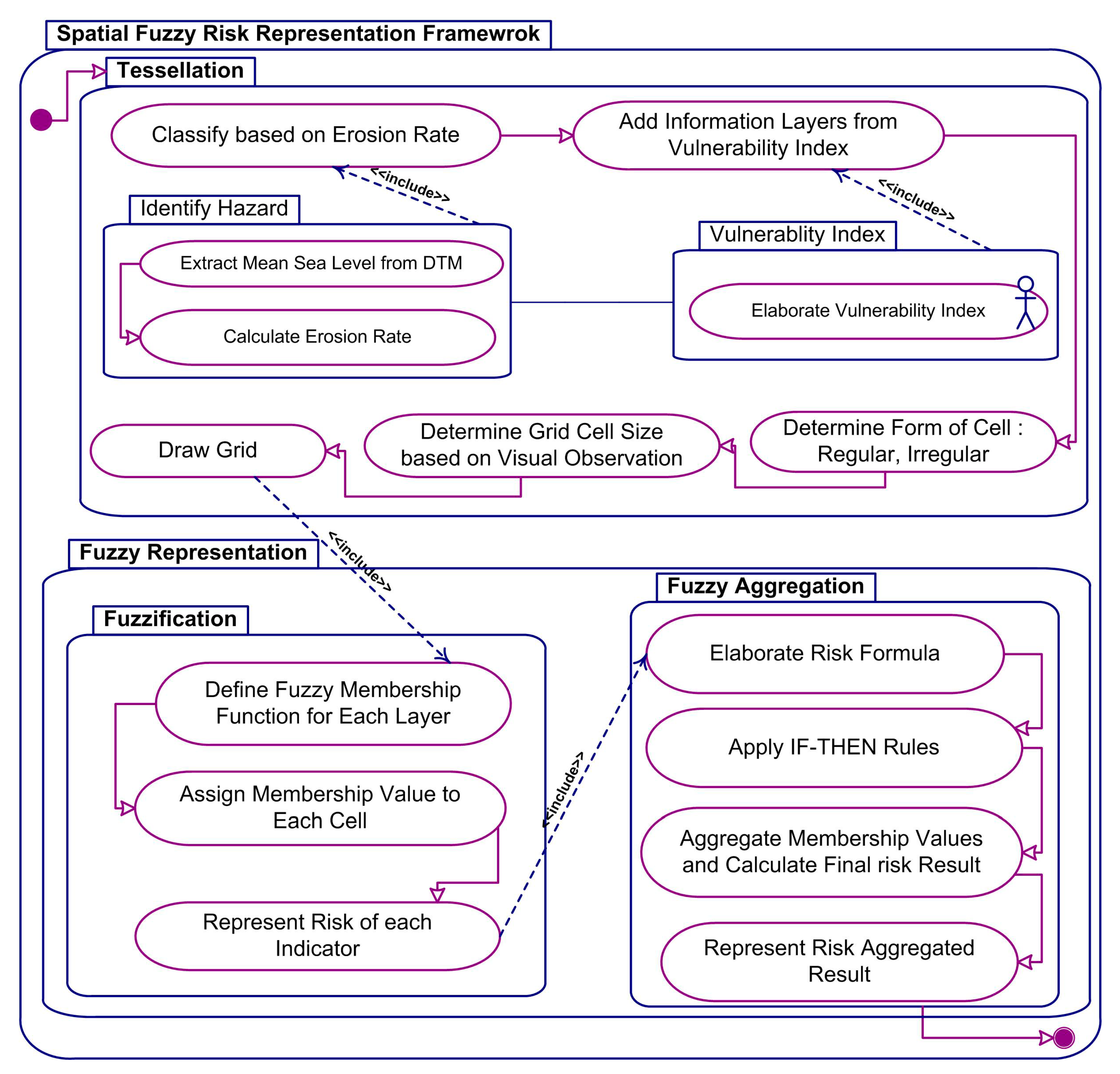
4. Fuzzy Representation of Coastal Erosion Risk: A Conceptual Framework


| 1. Draw the grid on the region with respect to the identified hazard and elaborated vulnerability index, |
| 2. For I = 1:number of vulnerable indicators, |
| a. For j = 1:length of the grid, |
| i. Determine the fuzzy membership value for each cell of the grid using defined fuzzy membership function of each indicator, |
| ii. Assign membership value to center of each cell for each indicator, |
| iii. Represent the risk value for each indicator, |
| b. End |
| 3. End |
| 4. Aggregate the risk value of different indicators based on assign operator, |
| i. Elaborate risk formula, |
| ii. Apply IF-THEN rules, |
| iii. Calculate the risk value, |
| 5. Represent the aggregated result, |
| 6. End. |
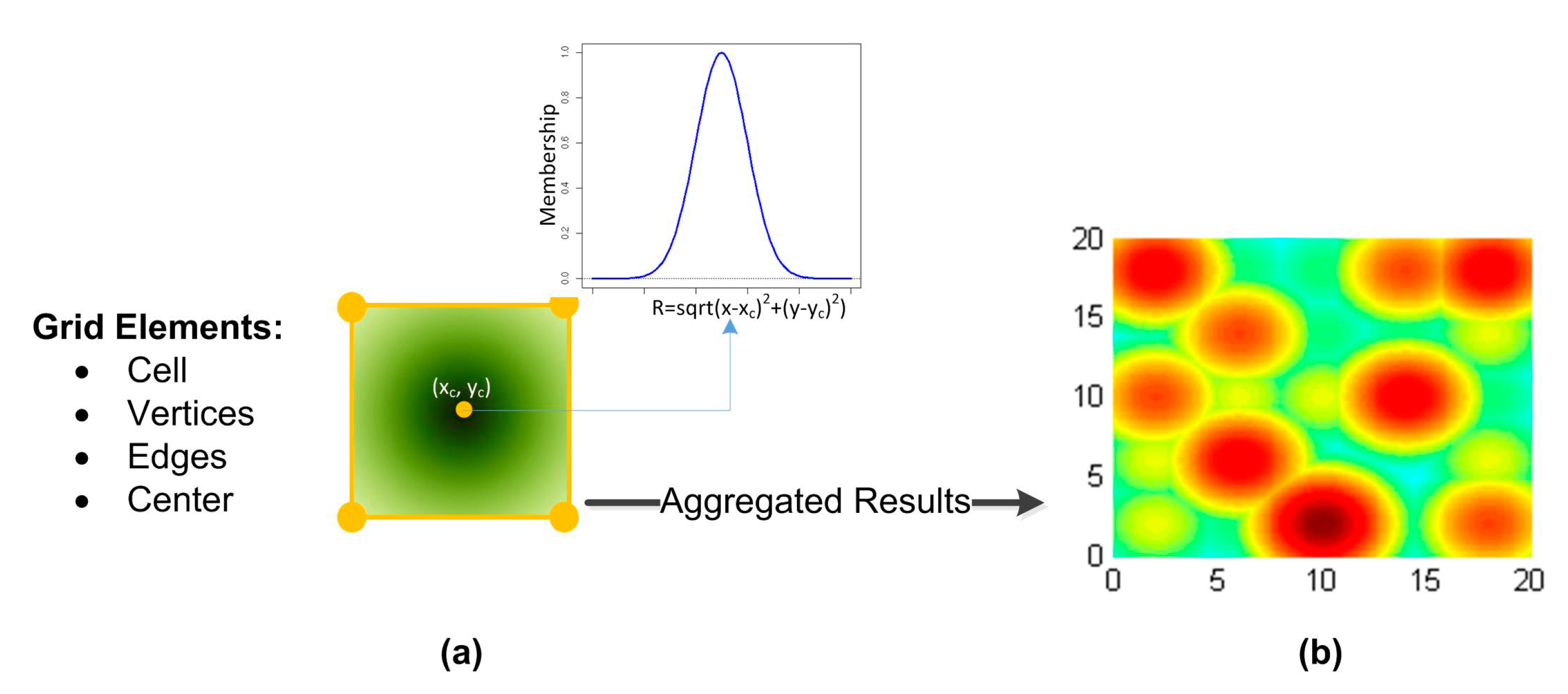
4.1. Tessellation

4.2. Fuzzy Representation
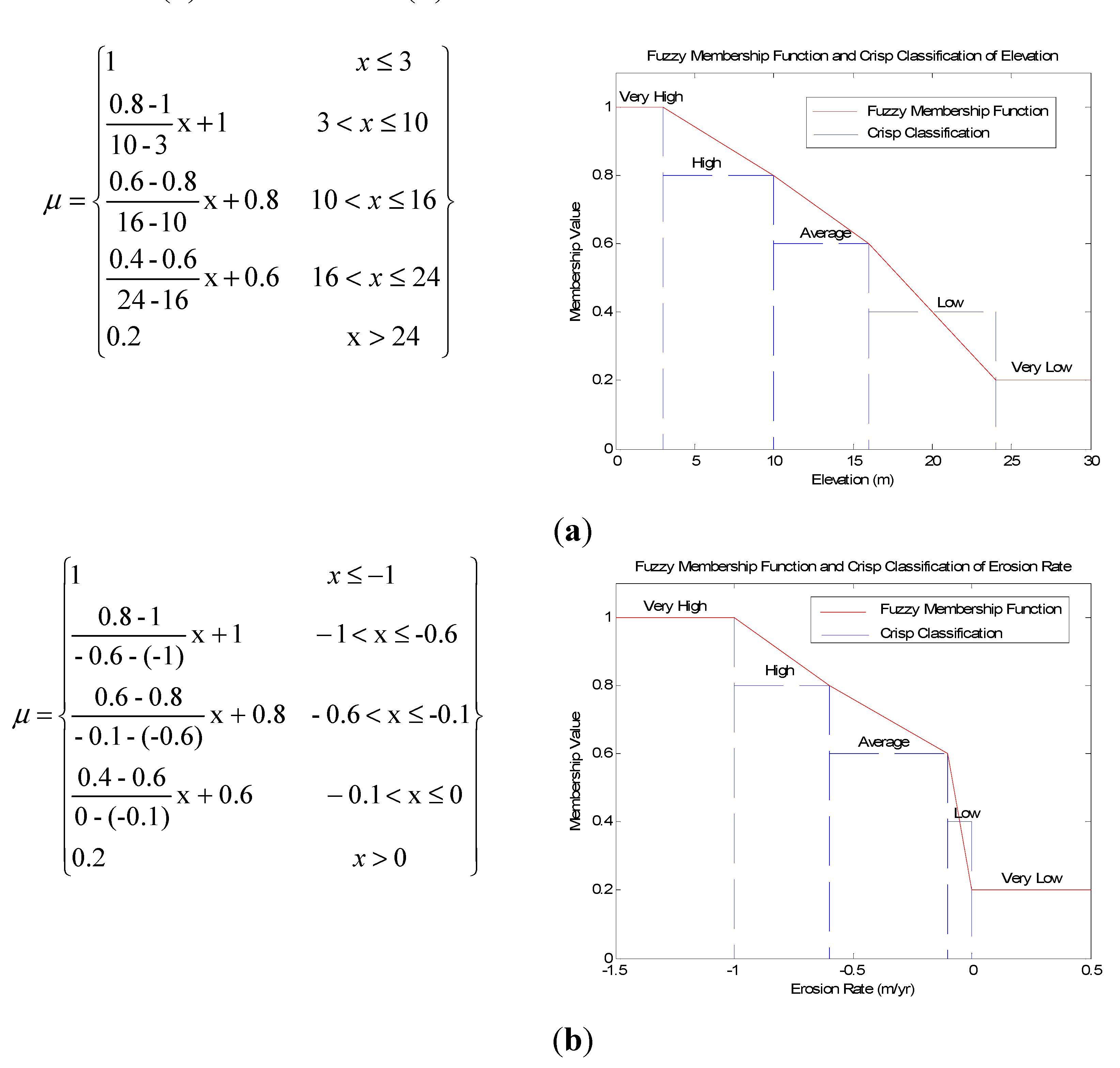
4.2.1. Fuzzification
 .
.


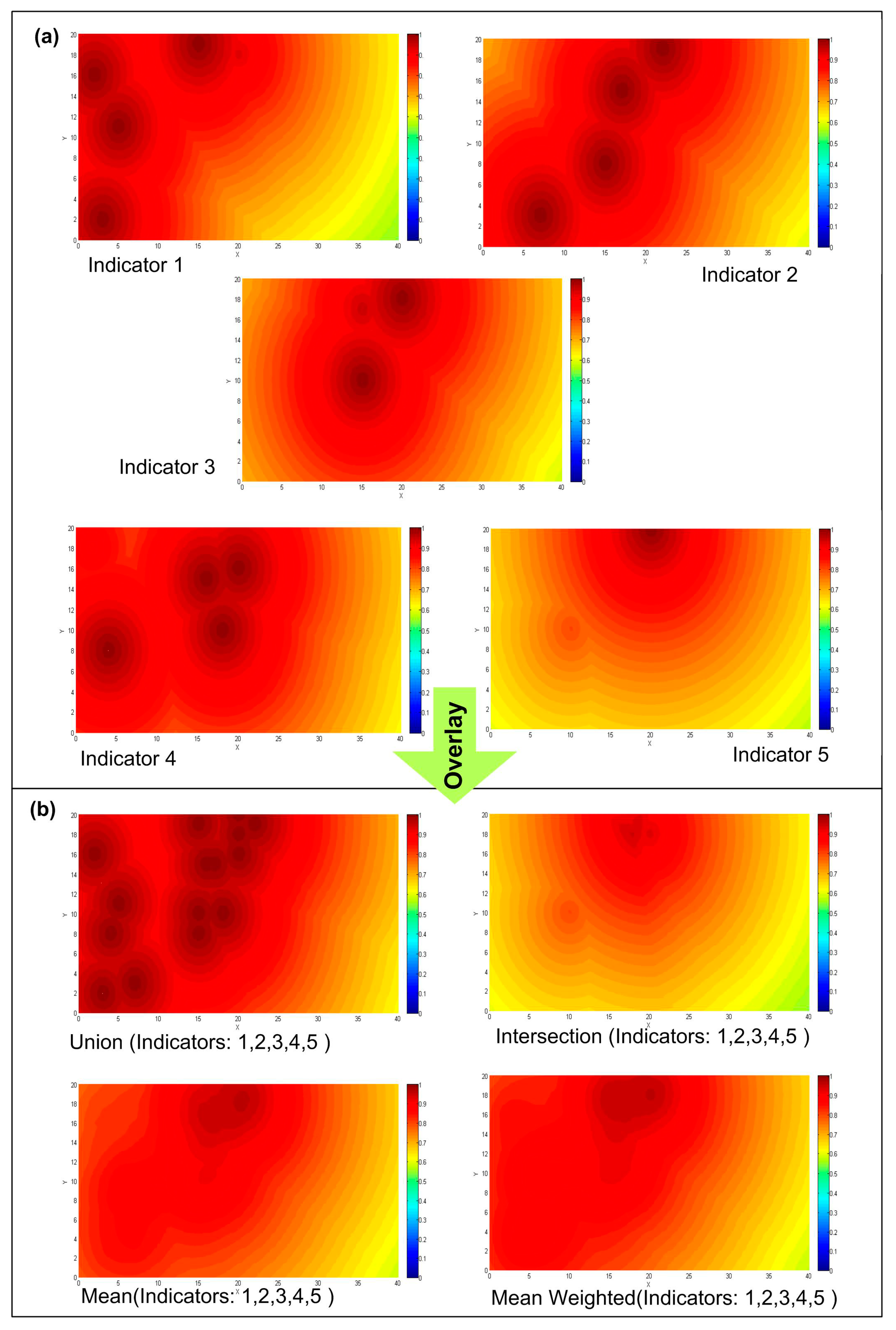
4.2.2. Fuzzy Aggregation
| IF (HydroNetwork is VH) and (ProtectStructure is VH) and (DistObjVul is VH) and (ErosionRate is H) |
| THEN (Use “MAX” operation for “Erosion Risk” calculation) |
| VH: very high, H: high, A: Average, L: low, VL: very Low |

| Linguistic Expression | Crisp Value | Fuzzy Risk Value |
|---|---|---|
| Very Low Risk of Erosion | Risk(Erosion) = 1 | 0 ≤ Risk(Erosion) ≤ 0.175 |
| Low Risk of Erosion | Risk(Erosion) = 2 | 0.175 < Risk(Erosion) ≤ 0.375 |
| Average Risk of Erosion | Risk(Erosion) = 3 | 0.375 < Risk(Erosion) ≤ 0.575 |
| High Risk of Erosion | Risk(Erosion) = 4 | 0.575 < Risk(Erosion) ≤ 0.775 |
| Very High Risk of Erosion | Risk(Erosion) = 5 | 0.775 < Risk(Erosion) ≤ 1 |
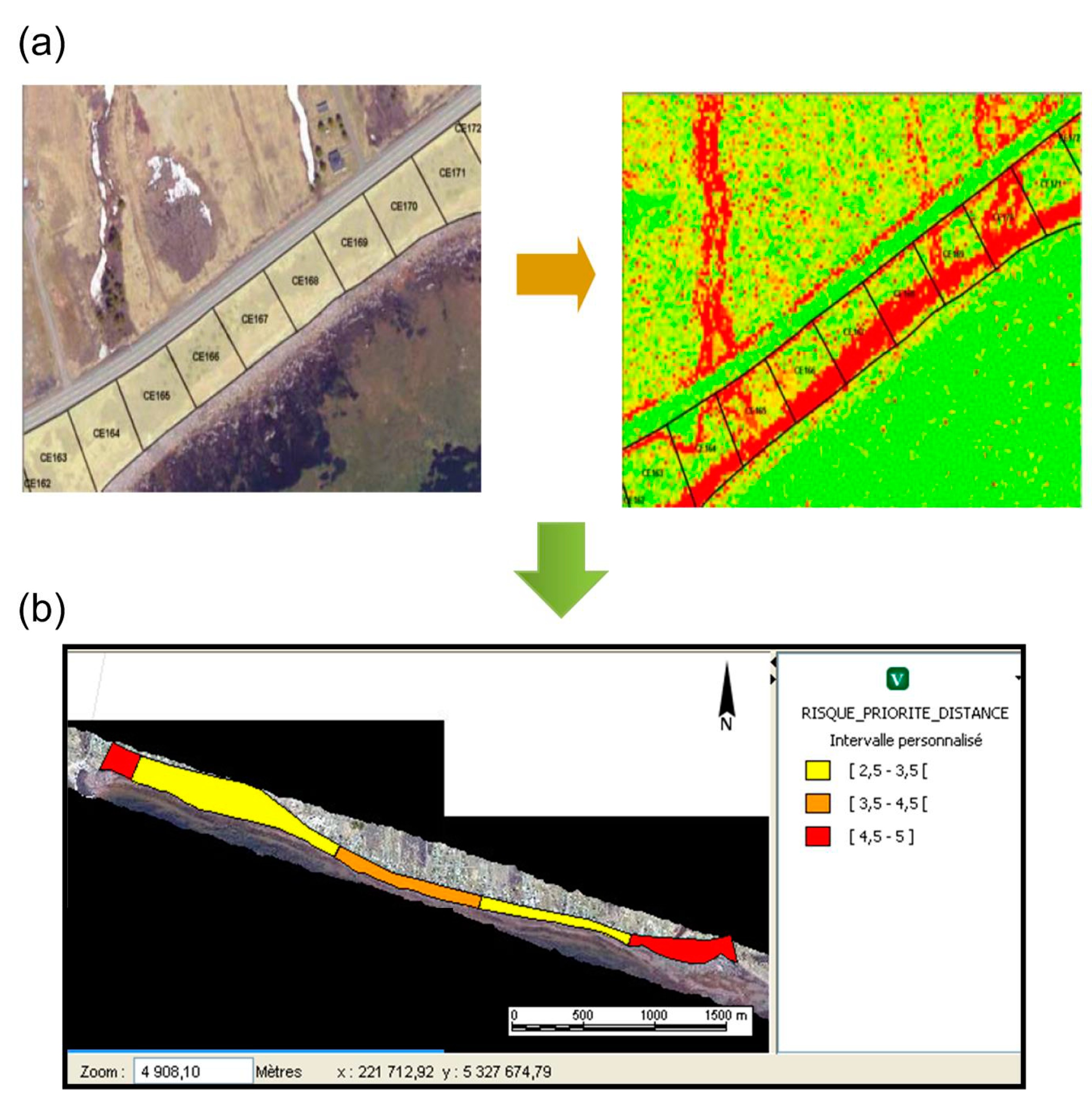
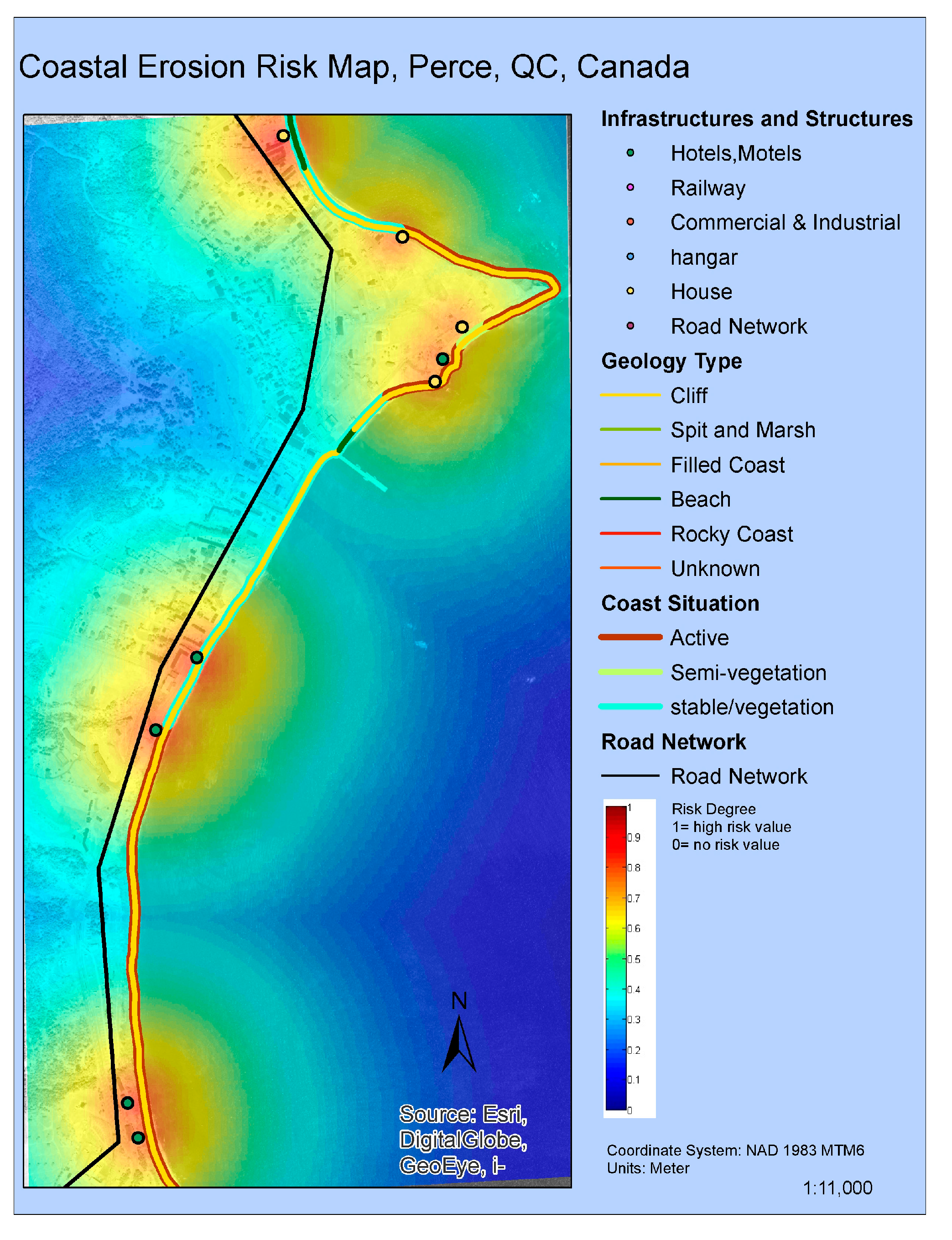
5. Results: A Case Study
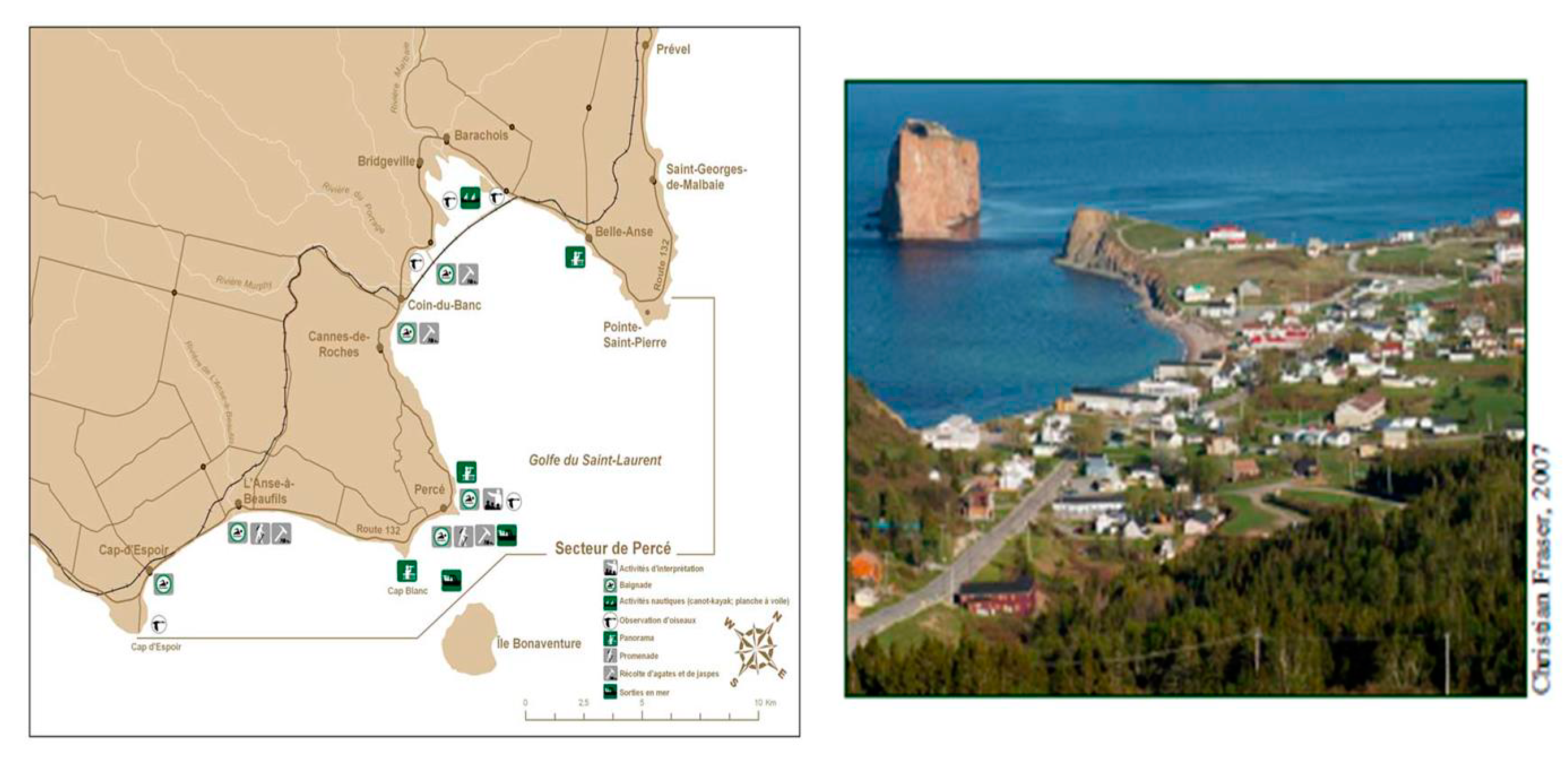
5.1. Study Site

5.2. Implementing Proposed Framework on Study Site
| Source | Extracted Information |
|---|---|
| LiDAR Data | Slop, DEM, erosion rate |
| Technical and Research Reports | Protection structure, Infrastructure situation, type of coastline, state of coastline, land use information, distance coast and 5 m depth, distance coast element at risk |
| Geobase | Hydrology network and drainage, land use |
| Quebec Prov. Transport Dept. | Road network |

| Risk Parameters | Weight (wt) | Membership Function |
| Protection Structure | 34% |  |
| Distance coast and element at risk | 17% |  |
| Mean Slop | 13% |  |
| DEM | 10% |  |
| Geology Type | 8% |  |
| Land Cover | 7% |  |
| Hydrology Network | 6% |  |
| Distance coast to 5 m depth | 5% |  |
| Erosion Rate |  |

5.3. Results Interpretation
6. Discussion and Remarks
- Spatial uncertainty associated with object definition is explicitly dealt with through the fuzzy approach. It is also possible to attach a probability density to the values of position and measurement uncertainty. If this is the case, before using this data in CERA, cleaning the data using probability approaches with an accepted confidence level is recommended.
- Membership function definition issues are resolved by converting the crisp classification of vulnerability index to a fuzzy classification. Accordingly, the integration of multiple criteria is performed by aggregating their respective membership values using fuzzy aggregation operators. If the vulnerability index classification is not available, methods such as Fuzzy C-Mean and Fuzzy K-Mean are recommended to define the required membership functions based on available data.
- Elaborating risk formula and then constructing IF-THEN rules of associated indicators allows direct control over the entire CERA process. In addition, this provides more flexibility if one or more indicators or their classifications are changed. In this case, updating the desired information by re-running the fuzzification step or modifying the IF-THEN rules by re-executing the fuzzy aggregation step will be sufficient.
- The proposed approach allows performing multiple fuzzy aggregation operators (union, intersection, mean, mean weighted) that is required in any CERA process. The result in Figure 7b shows how significantly the choice of fuzzy operators can affect the end result. Therefore, with regards to the needs of decision makers and the emergence of protection actions, the choice of these operators is also varied.
- The flexibility of fuzzy set theory to characterize and handle inherent spatial uncertainty through the entire assessment process widely increases the confidence levels of adapted strategies for protection regions under study. It also accelerates the implementation of response plans in case of a disaster through the interpretation of the results and the prioritization of planning actions based on expert perception. From another point of view, traditional risk assessment methods lead to crisp decisions, i.e., “Yes” or ”No” while the fuzzy approach leads to smooth transitions between these two extremes.
- Fuzzy risk representation is a relatively new concept for decision makers. In this new context, decision-making processes need to be adapted and meaningful criteria need to be established to accept and manipulate fuzzy risk values. Changing the decision making culture to use fuzzy results requires finding evidence to convince the decision makers of the benefits of this new approach. The defuzzification step explained briefly in this paper is an alternative in this regard to translate fuzzy values to measurable values, making them understandable for decision makers. Kentel and Aral [2] propose a risk-tolerance measure method based on a crisp compliance guideline, which is already available in some domains, such as the health system.
- The proposed fuzzy representation is tested only on regular tessellation. The neighborhood relation is implicit, based on the ID of a cell. If an irregular tessellation is needed, more effort in neighborhood concepts and topological predicates are required.
- The temporal aspect of the fuzzy object is not taken into account in this approach. This paper only discusses the spatial extent of fuzzy objects and the situations in which the fuzzy classification is due to the multi-criteria nature of CERA and spatial uncertainty associated with object definition. This means that the risk zones are represented spatially as a snapshot of a given time period. How to handle fuzzy objects that change in different time periods needs more investigation.
- The proposed approach is employed only on a small region with a given level of detail (scale). When the analysis of extremely large amounts of data within a hierarchical system is required, the proposed approach needs to be adjusted with respect to selected technology. In this regard, efforts are mainly needed on fuzzy aggregation operators such as “Fusion” where the multi-scale representation is required.
7. Conclusions
Acknowledgments
Author Contributions
Conflicts of Interest
References
- Darbra, R.; Eljarrat, E.; Barceló, D. How to measure uncertainties in environmental risk assessment. TrAC Trends Anal. Chem. 2008, 27, 377–385. [Google Scholar] [CrossRef] [Green Version]
- Kentel, E.; Aral, M.M. Risk tolerance measure for decision-making in fuzzy analysis: A health risk assessment perspective. Stoch. Environ. Res. Risk Assess. 2007, 21, 405–417. [Google Scholar] [CrossRef]
- Xie, Y.; Yi, S.; Cao, Y.; Lu, Y. Uncertainty information fusion for flood risk assessment based on DS-AHP method. In Proceedings of the 19th International Confrence on Geoinformatics, Shanghai, China, 24–26 June 2011; pp. 1–6.
- Dolan, A.; Walker, I. Understanding vulnerability of coastal communities to climate change related risks. J. Coast. Res. 2006, SI 39, 1317–1324. [Google Scholar]
- Jadidi, A.; Mostafavi, M.A.; Bédard, Y.; Long, B.; Grenier, E. Using geospatial business intelligence paradigm to design a multidimensional conceptual model for efficient coastal erosion risk assessment. J. Coast. Conserv. 2013, 17, 527–543. [Google Scholar] [CrossRef]
- Boruff, B.; Cutter, S.; Emrich, C. Erosion hazard vulnerability of US coastal counties. J. Coast. Res. 2005, 21, 932–942. [Google Scholar] [CrossRef]
- Walker, W.; Rotmans, J.; Vander Sluijs, J.; van Assel, T.; Janssesn, P.; Krayer von Krauss, M.; Harremoees, P. Defining uncertainty a conceptual basis for uncertainty management in model-based decision support. Integr. Assess. 2003, 4, 5–17. [Google Scholar] [CrossRef]
- Zadeh, L.A. Toward a generalized theory of uncertainty (GTU)––An outline. Inf. Sci. (N. Y.) 2005, 172, 1–40. [Google Scholar] [CrossRef]
- Fisher, P.; Comber, A.; Wadsworth, R. Approaches to uncertainty in spatial data. In Fundamentals of Spatial Data Quality; Devillers, R., Jeansoulin, R., Eds.; ISTE Ltd.: London, UK, 2010; Volume 1, pp. 43–59. [Google Scholar]
- Smith, B.; Varzi, A.C. Fiat and bona fide boundaries. Philos. Phenomenol. Res. 2000, 60, 401. [Google Scholar] [CrossRef]
- Smith, B.; Mark, D.D.M. Do mountains exist? Towards an ontology of landforms. Environ. Plan. B Plan. Des. 2003, 30, 411–427. [Google Scholar] [CrossRef]
- McFadden, L.; Nicholls, R.J.; Vafeidis, A.T.; Tol, R.S.J. A methodology for modeling coastal space for global assessment. J. Coast. Res. 2007, 23, 911–920. [Google Scholar]
- Cheng, T.; Molenaar, M.; Stein, A. Fuzzy approach for integrated coastal zone management. In Remote Sensing and Geospatial Technologies for Coastal Ecosystem Assessment and Management; Yang, X., Ed.; Springer: Berlin/Heidelberg, Germany, 2009; pp. 67–90. [Google Scholar]
- Aerts, J.; Goodchild, M.F.; Heuvelink, G. Accounting for spatial uncertainty in optimization with spatial decision support systems. Trans. GIS 2003, 7, 211–230. [Google Scholar]
- Choa, H.-N.; Choi, H.-H.; Kim, Y.-B. A risk assessment methodology for incorporating uncertainties using fuzzy concepts. Reliab. Eng. Syst. Saf. 2003, 78, 173–183. [Google Scholar]
- Cowell, P.; Zeng, T. Integrating uncertainty theories with GIS for modeling coastal hazards of climate change. Mar. Geod. 2003, 26, 5–18. [Google Scholar] [CrossRef]
- Fisher, P.; Cheng, T.; Wood, J. Higher order vagueness in geographical information: Empirical geographical population of type n fuzzy sets. Geoinformatica 2007, 11, 311–330. [Google Scholar] [CrossRef]
- Pauly, A.; Schneider, M. VASA: An algebra for vague spatial data in databases. Inf. Syst. 2010, 35, 111–138. [Google Scholar] [CrossRef]
- Schneider, M. Design and implementation of finite resolution crisp and fuzzy spatial objects. Data Knowl. Eng. 2003, 44, 81–108. [Google Scholar] [CrossRef]
- Schneider, M. Vague spatial data types. Adv. Spat. Databases Lect. Notes Comput. Sci. 2003, 44, 81–108. [Google Scholar]
- Dilo, A.; de By, R.A.; Stein, A. A system of types and operators for handling vague spatial objects. Int. J. Geogr. Inf. Sci. 2007, 21, 397–426. [Google Scholar] [CrossRef]
- Kanjilal, V.; Liu, H.; Schneider, M. Plateau regions: An implementation concept for fuzzy regions in spatial databases and GIS. In Proceedings of the 13th International Conference on Information Processing and Management of Uncertainty in KnowledgeBased Systems, Dortmund, Germany, 28 June–2 July 2010; Volume 6178 LNAI, pp. 624–633.
- Bejaoui, L.; Pinet, F.; Salehi, M.; Schneider, M.; Bédard, Y. Logical consistency for vague spatiotemporal objects and relations. In Proceedings of 5th International Symposium Spatial Data Quality 2007, ITC, Enschede, The Netherlands, 13–15 June 2007.
- Cohn, A.; Hazarika, S. Qualitative spatial representation and reasoning: An overview. Fundam. Inf. 2001, 46, 1–29. [Google Scholar]
- Molenaar, M.; Cheng, T. Fuzzy spatial objects and their dynamics. ISPRS J. Photogramm. Remote Sens. 2000, 55, 164–175. [Google Scholar] [CrossRef]
- Fisher, P.; Cheng, T.; Wood, J. Fuzziness and ambiguity in multi-scale analysis of landscape morphometry. In Fuzzy Modeling with Spatial Information for Geographic Problems; Petry, F., Cobb, M.A., Robinson, V.B., Eds.; Springer: Berlin/Heidelberg, Germany, 2005; pp. 209–232. [Google Scholar]
- Goodchild, M.F.; Glennon, A. Representation and computation of geographic dynamics. In Understanding Dynamics of Geographic Domains; Hornsby, K., Yuan, M., Eds.; Taylor & Francis Group, LLC: London, UK, 2008; pp. 13–30. [Google Scholar]
- Vanneuville, W.; Maeghe, K.; Deschamps, M.; de Maeyer, P.; Mostaert, F.; de Rouck, K. Spatial calculation of flood damage and risk ranking. In Proceedings of the 8th Conference on Geographic Information Science, Estoril, Portugal, 26–28 May 2005; pp. 549–556.
- McHugh, R.-M.; Bilodeau, F.; Rivest, S.; Bédard, Y.; Michaud, M. Analyse du potentiel d’une application SOLAP pour une gestion efficace de l’érosion des berges en Gaspésie Iles-de-la-Madeleine. In Proceedings of Géomatique 2006, Montreal, QC, Canada, 25–26 October 2006.
- Bédard, Y. Uncertainties in land infromarion systems databases. In Auto-Carto; Chrisman, N., Ed.; American Society for Photogrammetry and Remote Sensing, American Congress on Surveying and Mapping: Baltimore, MD, USA, 1988; pp. 175–184. [Google Scholar]
- Fisher, P. Uncertainty, semantic. In Encyclopedia of GIS; Springer-Verlag: Berlin/Heidelberg, Germany, 2008; pp. 1194–1196. [Google Scholar]
- Dilo, A. Representation of and Reasoning with Vagueness in Spatial Information: A System for Handling Vague Objects. PhD Dissertation, ITC, Enschede, The Netherlands, 2006; p. 187. [Google Scholar]
- Robinson, V.B. A perspective on the fundamentals of fuzzy sets and their use in geographic information systems. Trans. GIS 2003, 7, 3–30. [Google Scholar]
- Burrough, P. Fuzzy mathematical methods for soil survey and land evaluation. J. Soil Sci. 1989, 40, 477–492. [Google Scholar] [CrossRef]
- Usery, E.L. A conceptual framework and fuzzy set implementation for geographic features. In Geographic Objects with Indeterminate Boundaries; Burrough, P., Frank, A., Eds.; Taylor & Francis: London, UK, 1996; pp. 71–87. [Google Scholar]
- Altman, D. Fuzzy set theoretic approaches for handling imprecision in spatial analysis. Int. J. Geogr. Inf. Sci. 1994, 8, 271–289. [Google Scholar] [CrossRef]
- Brown, D. Classification and boundary vaguen ess in mapping presettlement forest types. Int. J. Geogr. Inf. Sci. 1998, 12, 105–129. [Google Scholar] [CrossRef]
- Molenaar, M. Tree conceptual uncertainty levels for spatial objects. Int. Arch. Photogramm. Remote Sens. 2000, XXXIII, 670–677. [Google Scholar]
- Vassur, B.; Van De Vlag, D.; Stein, A.; Jeansoulin, R.; Dilo, A. Spatio-temporal ontology for defining the quality of an application. In Proceedings of ISSDQ, Bruck an der Leitha, Austria, 15–17 April 2004; p. 13.
- Cheng, T.; Fisher, P.; Li, Z. Double Vagueness: Effect of scale on the modelling of fuzzy spatial objects. In Developments in Spatial Data Handling; Pete, F., Ed.; Springer: Berlin/Heidelberg, Germany, 2005; pp. 299–313. [Google Scholar]
- Cheng, T. Fuzzy objects: Their CHanges and uncertainties. Photogramm. Eng. Remote Sens. 2002, 68, 41–49. [Google Scholar]
- Chen, K. Quantifying environmental attributes from Earth Observation data products by spatial upscaling: Three case studies. In Proceedings of the 2nd International Conference on Earth Observation for Global Changes (CD-ROM), Chengdu, China, 25–29 May 2009; pp. 1600–1610.
- Roy, P.; Mandal, J. A novel fuzzy-GIS model based on delaunay triangulation to forecast facility locations (FGISFFL). Int. Symp. Electron. Syst. Des. 2011, 48, 341–346. [Google Scholar]
- Dragicevic, S.; Marceau, D.J. Space, time, and dynamics modeling in historical GIS databases: A fuzzy logic approach. Environ. Plan. B Plan. Des. 2001, 28, 545–562. [Google Scholar] [CrossRef]
- Chowdhury, S.; Champagne, P.; McLellan, P.J. Uncertainty characterization approaches for risk assessment of DBPs in drinking water: A review. J. Environ. Manag. 2009, 90, 1680–1691. [Google Scholar] [CrossRef]
- Morris, A.; Jankowski, P. Spatial decision making using fuzzy GIS. In Fuzzy Modeling with Spatial Information for Geographic Problems; Petry, F., Cobb, M.A., Robinson, V.B., Eds.; Springer: Berlin/Heidelberg, Germany, 2005; pp. 275–298. [Google Scholar]
- Zadeh, L.A. Fuzzy set. Inf. Control 1965, 8, 338–353. [Google Scholar] [CrossRef]
- Zhan, F.B.; Lin, H. Overlay of two simple polygons with indeterminate boundaries. Trans. GIS 2003, 7, 67–81. [Google Scholar]
- Randell, D.; Cui, Z.; Cohn, A. A spatial logic based on regions and connection. In Proceedings of the International Conference on Knowledege Representation and Reasoning (Kr92); Nebel, B., Rich, C., Swartout, W., Eds.; Morgan Kaufmann: San Mateo, CA, USA, 1992; pp. 165–176. [Google Scholar]
- Erwig, M.; Schneider, M. Vague regions. In Advances in Spatial Databases; Scholl, M., Voisard, A., Eds.; Lecture Notes in Computer Science; Springer: Berlin/Heidelberg, Germany, 1997; Volume 1262, pp. 298–320. [Google Scholar]
- Schneider, M. Uncertainty management for spatial datain databases: Fuzzy spatial data types advances in spatial databases. In Proceedings of the 6th International Symposium Advances in Spatial Databases (SSD’99), Hong Kong, China, 20–23 July 1999; Güting, R., Papadias, D., Lochovsky, F., Eds.; Springer: Berlin/Heidelberg, Germany; Hong Kong, China, 1999; Volume 1651, pp. 330–351. [Google Scholar]
- Cheng, T.; Molenaar, M.; Lin, H. Formalizing fuzzy objects from uncertain classification results. Int. J. Geogr. Inf. Sci. 2001, 15, 27–42. [Google Scholar] [CrossRef]
- Tang, X. Spatial Object Modeling in Fuzzy Topological Spaces with Applications to Land Cover Change. PhD Dessertation, ITC, Enschede, The Netherlands, 2004; p. 241. [Google Scholar]
- Wang, F.; Hall, G.; Brent, H. Fuzzy representation of geographical boundaries in GIS. Int. J. Geogr. Inf. Sci. 1996, 10, 537–590. [Google Scholar]
- Bezdek, J.; Ehrlich, R.; Full, W. FCM: The fuzzy c-means clustering algorithm. Comput. Geosci. 1984, 10, 191–203. [Google Scholar] [CrossRef]
- Chi, Z.; Wu, J.; Yan, H. Handwritten numeral recognition using self-organizing maps and fuzzy rules. Pattern Recognit. 1995, 28, 59–66. [Google Scholar] [CrossRef]
- Mannan, B.; Roy, J.; Ray, A. Fuzzy ARTM AP supervised classification of multi-spectral remotely-sensed images. Int. J. Remote Sens. 1998, 19, 767–775. [Google Scholar] [CrossRef]
- Nauck, D.; Kruse, R. A neuro-fuzzy method to learn fuzzy classification rules from data. Fuzzy Sets Syst. 1997, 89, 277–288. [Google Scholar] [CrossRef]
- Genz, A.; Fletcher, C.; Dunn, R.; Frazer, L.; Rooney, J. The Predictive accuracy of shoreline change rate methods and alongshore beach variation on Maui, Hawaii. J. Coast. Res. 2007, 23, 87–105. [Google Scholar]
- Füssel, H.-M.; Klein, R.J. Climate change vulnerability assessments: An evolution of conceptual thinking. Clim. Chang. 2006, 75, 301–329. [Google Scholar] [CrossRef]
- Bejaoui, L. Qualitative Topological Relationships for Objects with Possibly Vague Shapes: Imolication on the Specification of Topological Integrity Constraint in Transactional Spatial Databases and in Spatial Data Warehouses. PhD Dessertation, Université Laval, Quebec City, QC, Canada, 2009; p. 246. [Google Scholar]
- StatisticCanada 2011 Census. Statistics Canada Catalogue no. 98–316-XWE. Census profile: Percé, Quebec (Code 2402005) and Quebec (Code 24). Available online: http://archive.today/f9I7o (accessed on 10 June 2012).
- Bernatchez, P.; Fraser, C.; Friesnger, S.; Jolivet, Y.; Dugas, S.; Drejza, S.; Morissette, A. Sensibilité des Côtes et Vulnérabilité des Communautés du Golfe du Saint-Laurent aux Impacts des Changements Climatiques; Laboratoire de Dynamique et de Gestion Intégrée des Zones Côtières, UQAR: Rimouski, Canada, 2008; p. 256. [Google Scholar]
- Bernatchez, P.; Fraser, C.; Lefaivre, D. Effets des structures rigides de protection sur la dynamique des risques naturels côtiers: Érosion et submersion. In Proceedings of the 4th Canadian Conference on Geohazard: From Causes to Managment, Universite Laval, Quebec City, QC, Canada, 20–24 May 2008; Locat, J., Perret, D., Turmel, D., Demers, D., Leroueil, S., Eds.; pp. 594–604.
- Thieler, E.; Zichichi, J.; Ergul, A.; Himmelstoss, A. Digital Shoreline Analysis System (DSAS) version 4.0—An ArcGIS Extension for Calculating Shoreline Change; U.S. Geological Survey Open-File Report 2008–1278; U.S. Geological Survey: Woods Hole, MA, USA, 2009; p. 33. [Google Scholar]
- Xhardé, R. Application des Techniques Aéroportées Vidéographiques et Lidar à L’étude des Risques Naturels en Milieu Côtier. PhD Dessertation, INRS, Quebec City, QC, Canada, 2007; p. 283. [Google Scholar]
© 2014 by the authors; licensee MDPI, Basel, Switzerland. This article is an open access article distributed under the terms and conditions of the Creative Commons Attribution license (http://creativecommons.org/licenses/by/3.0/).
Share and Cite
Jadidi, A.; Mostafavi, M.A.; Bédard, Y.; Shahriari, K. Spatial Representation of Coastal Risk: A Fuzzy Approach to Deal with Uncertainty. ISPRS Int. J. Geo-Inf. 2014, 3, 1077-1100. https://doi.org/10.3390/ijgi3031077
Jadidi A, Mostafavi MA, Bédard Y, Shahriari K. Spatial Representation of Coastal Risk: A Fuzzy Approach to Deal with Uncertainty. ISPRS International Journal of Geo-Information. 2014; 3(3):1077-1100. https://doi.org/10.3390/ijgi3031077
Chicago/Turabian StyleJadidi, Amaneh, Mir Abolfazl Mostafavi, Yvan Bédard, and Kyarash Shahriari. 2014. "Spatial Representation of Coastal Risk: A Fuzzy Approach to Deal with Uncertainty" ISPRS International Journal of Geo-Information 3, no. 3: 1077-1100. https://doi.org/10.3390/ijgi3031077