A Concept for Uncertainty-Aware Analysis of Land Cover Change Using Geovisual Analytics

Abstract

Analysis of land cover change is one of the major challenges in the remote sensing and GIS domain, especially when multi-temporal or multi-sensor analyses are conducted. One of the reasons is that errors and inaccuracies from multiple datasets (for instance caused by sensor bias or spatial misregistration) accumulate and can lead to a high amount of erroneous change. A promising approach to counter this challenge is to quantify and visualize uncertainty, i.e., to deal with imperfection instead of ignoring it. Currently, in GIS the incorporation of uncertainty into change analysis is not easily possible. We present a concept for uncertainty-aware change analysis using a geovisual analytics (GVA) approach. It is based on two main elements: first, closer integration of change detection and analysis steps; and second, visual communication of uncertainty during analysis. Potential benefits include better-informed change analysis, support for choosing change detection parameters and reduction of erroneous change by filtering. In a case study with a change scenario in an area near Hamburg, Germany, we demonstrate how erroneous change can be filtered out using uncertainty. For this, we implemented a software prototype according to the concept presented. We discuss the potential and limitations of the concept and provide recommendations for future work.

1. Introduction

Uncertainty is inherent in geospatial data and can have severe impacts on spatiotemporal analysis [1]. However, it is still common to assume that data is error free although it has been shown that “[e]rror-laden data, used without consideration of their intrinsic uncertainty, are highly likely to lead to information of dubious value” (p.3). This is especially true for change detection and analysis since multiple remote sensing (RS) scenes are involved. Uncertainty accumulates over the scenes and further uncertainty is introduced, e.g., during the classification step in post-classification change detection. Thus, analysis of detected change has to cope with a high degree of uncertainty. Sensitivity analyses, performed by Pontius and Lippitt, demonstrated that half of all detected “changes” were caused by errors, although the overall accuracy for each of the input data sets was determined to be 91% [2]. This is one of the reasons why we see the need for a concept to incorporate uncertainty into change analysis instead of just ignoring it.

Traditionally, GIS are created to utilize precise geodata, which makes it difficult to use them for uncertainty-aware analysis. One reason for this is that uncertainty is stored as a separate data layer and not as an integrated part of a dataset. Another reason is that change detection and the analysis of changes are conducted as separate steps (Figure 1). In the past, much effort was devoted to enhancing the detection step, often with the goal of full automation [3]. We follow a different approach and suggest a closer integration of the change detection and analysis steps and the incorporation of uncertainty through visualization.

This article is structured as follows: we introduce the concept in Section 2, focusing on geovisual analytics and on a measure for change uncertainty. Possible applications are presented in Section 3. In Section 4, a case study shows how the concept can be implemented and discusses the potential benefits and drawbacks. From this, we derive a conclusion and provide an outlook on future work in Section 5.

Figure 1. Common workflow including change detection and analysis as separate steps.

Figure 1. Common workflow including change detection and analysis as separate steps.

2. Concept

In this section we present a concept to counter the challenges in change analysis described in Section 1. The basic idea is to facilitate uncertainty-aware change analysis by using iterative workflows with a high degree of user interaction. In the following subsections we introduce the concept following a geovisual analytics (GVA) approach and define an uncertainty measure for post-classification change.

2.1. Geovisual Analytics

We propose a geovisual analytics (GVA) approach to deal with the challenges discussed above. GVA is an interdisciplinary field following a “new paradigm for how information technologies can be used to process complex geospatial information to facilitate decision making, problem solving, and insight into geographical situations” [4] (p. 23). GVA “integrates perspectives from Visual Analytics (grounded in Information and Scientific Visualization) and Geographic Information Science (growing particularly in work concerning geovisualization, geospatial semantics and knowledge management, geocomputation, and spatial analysis)” [5] (p. 174). By integrating algorithms and user input with the help of visual interfaces, GVA tools establish the “linkage of visual and computational methods and tools for extracting hypotheses and information from spatial data” [6] (p.126). GVA is based on Visual Analytics that has successfully been used in other fields such as health research [7] or financial analysis [8], where neither automated nor manual analysis alone can provide the needed insight.

This research builds upon related work from two different categories: first, visual tools which make uncertainty usable in the analysis of RS data; and second, change analysis through visual analysis/analytics. Most work from the first category focuses on the classification of RS data, for example, a visual tool by Arko Lucieer named Parbat supports the optimization of segmentation parameters by visualizing uncertainty during classification [9]. Other work deals with the enhancement of class definitions, e.g., Ahlqvist used visualization of semantic similarity and overlap between class definitions to address incompatibilities of class definitions for land cover and land use [10]. Based on the work from the FLIERS project (Fuzzy Land Information from Environmental Remote Sensing), Bastin et al. developed a toolkit named VTBeans to enhance the classification of RS data with the help of uncertainty [11]. Multiple linked views can be combined to visualize uncertainty from different sources and, for instance, explore fuzzy spectral signatures to enhance class definitions.

In the second category regarding visual change analysis from RS data, there have also been a number of promising approaches that serve as a basis for our work. Zurita-Milla et al. extended the GIS software package ILWIS (Integrated Land and Water Information System) by adding a toolbox called SITS (Satellite Image Time Series) [12]. It facilitates the use of animation and interaction to analyze changes based on the imagery and provides filtering and aggregation functionality to conduct analyses at different levels of granularity. Another example is Change Matters, a web-based application for interactive change analysis of Landsat satellite imagery [13]. A change overlay is displayed on top of the imagery and the user can modify thresholds, e.g., for vegetation gain and loss. Based on this, change maps can be created interactively and distributed over the Internet. An interesting approach for multi-temporal change analysis was presented by Hoeber et al. They use spatiotemporal difference graphs to display change over multiple time points in GTDiff, a system that facilitates interactive exploration of multi-temporal changes [14].

All in all, there has been substantial work regarding the use of visual analysis and GVA to either explore uncertainty in geospatial data or to analyze change visually without incorporating uncertainty. However, we see the need for a concept that integrates the two approaches, merging the strengths of GVA and uncertainty visualization. Thus, the first goal of this concept is to use GVA to integrate detection and analysis of change and the second goal is to use potential benefits of uncertainty by visually communicating this information during analysis.

For a systematic design and documentation of workflows we created a workflow description concept in the form of a graph. It contains the following categories (Figure 2):

• Data: The data used during analysis (e.g., RS imagery, GIS layers, etc.)
• User: User interaction (e.g., choosing a threshold)
• Hypothesis: A hypothesis about change (e.g., “this area was falsely detected as change”)
• Computation: Computational steps in the workflow (e.g., classification of RS data)
• Visualization: Visual communication to the user (e.g., display of change uncertainty in a map)
• Result: The resulting change set

As already mentioned, the core of this concept is the combination of automated algorithms (“Computation”) and visual interfaces (“Visualization”). In close interplay with these two components the user generates hypotheses, evaluates their plausibility with the help of visualization tools and revises them iteratively. When the user confirms a hypothesis the end results can be exported. Example workflow descriptions are provided in Section 3.

Figure 2. Basic concept of iterative analysis facilitating geovisual analytics.

Figure 2. Basic concept of iterative analysis facilitating geovisual analytics.

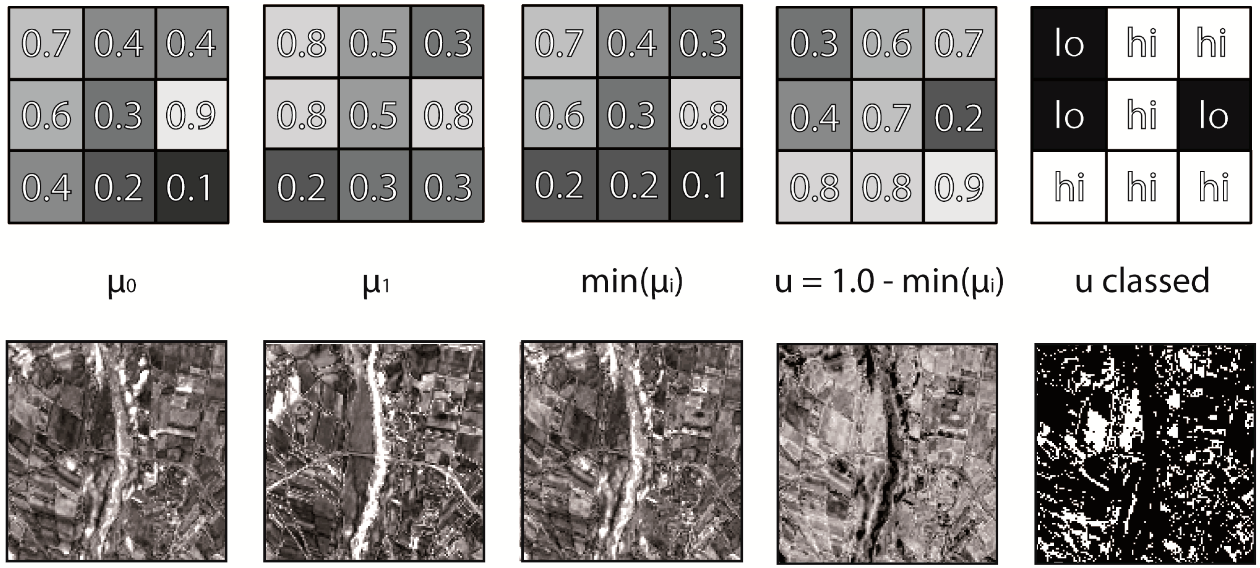
2.2. Change Uncertainty

Change detection based on remotely sensed data typically involves a high degree of uncertainty. Ignoring this fact can make further analysis of changes questionable [2]. During change detection, uncertainty from multiple RS scenes (errors and inaccuracies from sensor bias, misregistration, etc.) accumulate during the process, especially when multi-temporal (including more than two scenes) or multi-sensoral (using data from different sensors) detection is applied.

In the field of RS and GIS, research on modeling uncertainty in geospatial data has been conducted for decades. Different types of uncertainty (e.g., attribute, positional, and temporal) and their formal descriptions have been discussed in literature [1,15,16]. Substantial work regarding the description of uncertainty in land cover change was provided by Fisher and colleagues [17]. They extended the widely used change matrix to include fuzzy change values and provided a model for describing change uncertainty. Using a case study, they highlighted how fuzzy change data can reveal subtle changes that would not have been detectable with boolean change detection. At the same time they pointed out that “[w]hether the fuzzy mappings better reflect the landscape character than the Boolean remains an open question, and as is the reality of the differences noted here between the Boolean and fuzzy matrices of real change.” [17] (p.176). Generally, there are at least three ways to quantify uncertainty in land cover change:

• from accuracy assessment (class-specific) [1],
• from classification confidence, e.g., class membership probabilities (pixel-/object-specific) [18], and,
• from expert knowledge, e.g., estimation of class similarities (class-specific) [19].

Since our goal is to depict geographically varying uncertainty, class-specific measures are not taken into account since they only provide one uniform uncertainty value for all instances (pixels or objects) of a change type. Thus, we focused on uncertainty measures that are quantified by classification confidence. Based on the work by Fisher and his colleagues, we defined a straightforward uncertainty measure for land cover change on the basis of fuzzy membership values. The intersection of membership values μ_i from each scene is conducted by applying the minimum operator [17]. The complement of the minimum membership value yields a value for change uncertainty:

$$u=1.0-\min \left({\mu }_i\right)\text{ with }{\mu }_i\in \left[0.0, 1.0\right]$$

(1)

Figure 3. Example for change uncertainty measure (here: per-pixel and bi-temporal). Schematic (top row) and real data example (bottom row). Uncertainty is represented by a grayscale from black (0.0) to white (1.0).

Figure 3. Example for change uncertainty measure (here: per-pixel and bi-temporal). Schematic (top row) and real data example (bottom row). Uncertainty is represented by a grayscale from black (0.0) to white (1.0).

This uncertainty measure ranges from 0.0 (no uncertainty) to 1.0 (maximum uncertainty). It is straightforward to compute and can be applied to different spatial units (pixels, objects) and to any number of scenes (two or more). It is a compound measure reflecting uncertainty from all scenes resulting from errors and inaccuracies in the imagery, vagueness in land cover class definitions, ambiguity in class determination during classification, etc. Figure 3 illustrates the computation of the measure for two RS datasets, 0 and 1, in a schematic way (top row) and with real data (bottom row). The first two columns show the membership values of each dataset followed by the minimum membership values from both datasets. Subtraction from 1.0 yields the magnitudes of uncertainty. An exemplary division into two classes, “high” and “low”, is provided in the last column. This is an optional step, but in many cases unclassified uncertainty data may be too complex to interpret. A suitable number of uncertainty classes may depend on the task, yet for many applications two classes, i.e., “low uncertainty” and “high uncertainty”, will suffice. An alternative is percentage steps, for instance, the use of the three classes 0%, 50%, and 100%.

3. Applications

As already mentioned, we see several potential benefits of incorporating uncertainty in change analysis. In the following we discuss three specific applications to illustrate this: enabling a better informed analysis of detected change, optimizing the parameters used for change detection, and filtering by uncertainty to reduce false-positive change.

3.1. Enable Better Informed Analysis

When a human analyst explores change detection results, he or she creates hypotheses about land cover change. For instance, when informal settlements have been detected from satellite imagery the analyst may come up with the hypothesis that a specific settlement has grown over time. However, informal settlements are usually hard to delineate and have fuzzy boundaries, therefore the exact size of a detected settlement cannot be determined. In such cases, change uncertainty can provide further information to help interpret the detected change. For instance, a detected informal settlement may show lower uncertainty in its interior (making this part more reliable) and higher uncertainty at its boundaries, where a transition zone towards formal urban settlements may exist. When the analyst wants to determine the area of a settlement (and the number of people living there) uncertainty can provide information about the range of possible locations of the area’s boundary and thus can help derive a better estimate of the actual area. This way, information about uncertainty can make a hypothesis better defined and more plausible.

3.2. Optimize Change Detection Parameters

Another application of uncertainty that can potentially help with analyzing change is the optimization of the parameters used for its detection. With post-classification change detection, which we focus on here, the reliability of detected changes is highly dependent on the quality of the individual classifications on which the change detection step is based on. It was shown that misclassification can greatly impact change error [20]. Thus, often the only way to minimize change error is to increase the quality of the classified datasets. However, the optimization of classification parameters is not trivial and iterative modifications of the parameters are necessary to find a reasonable parameter set. To support this process, information on change uncertainty can help. The workflow depicted in Figure 4 shows that the user can visually explore a result after the initial classification of the single scenes and the change detection step. While iteratively modifying the parameters, the analyst gets immediate visual feedback on the resulting classified datasets and, thus, the detected changes. When the outcome is satisfying the current changes can be exported as final results. During the process, it is also possible to show the results for different parameter sets simultaneously so that the analyst is able to compare them and pick the best set.

This workflow is also applicable to other change detection approaches, e.g., when image differencing or ratioing are conducted, a threshold between change and no-change must be defined. In an analogous way, as described above, the choice of the change threshold can be optimized iteratively.

Figure 4. Workflow: Optimizing change parameters.

Figure 4. Workflow: Optimizing change parameters.

3.3. Reduce False-Positive Change

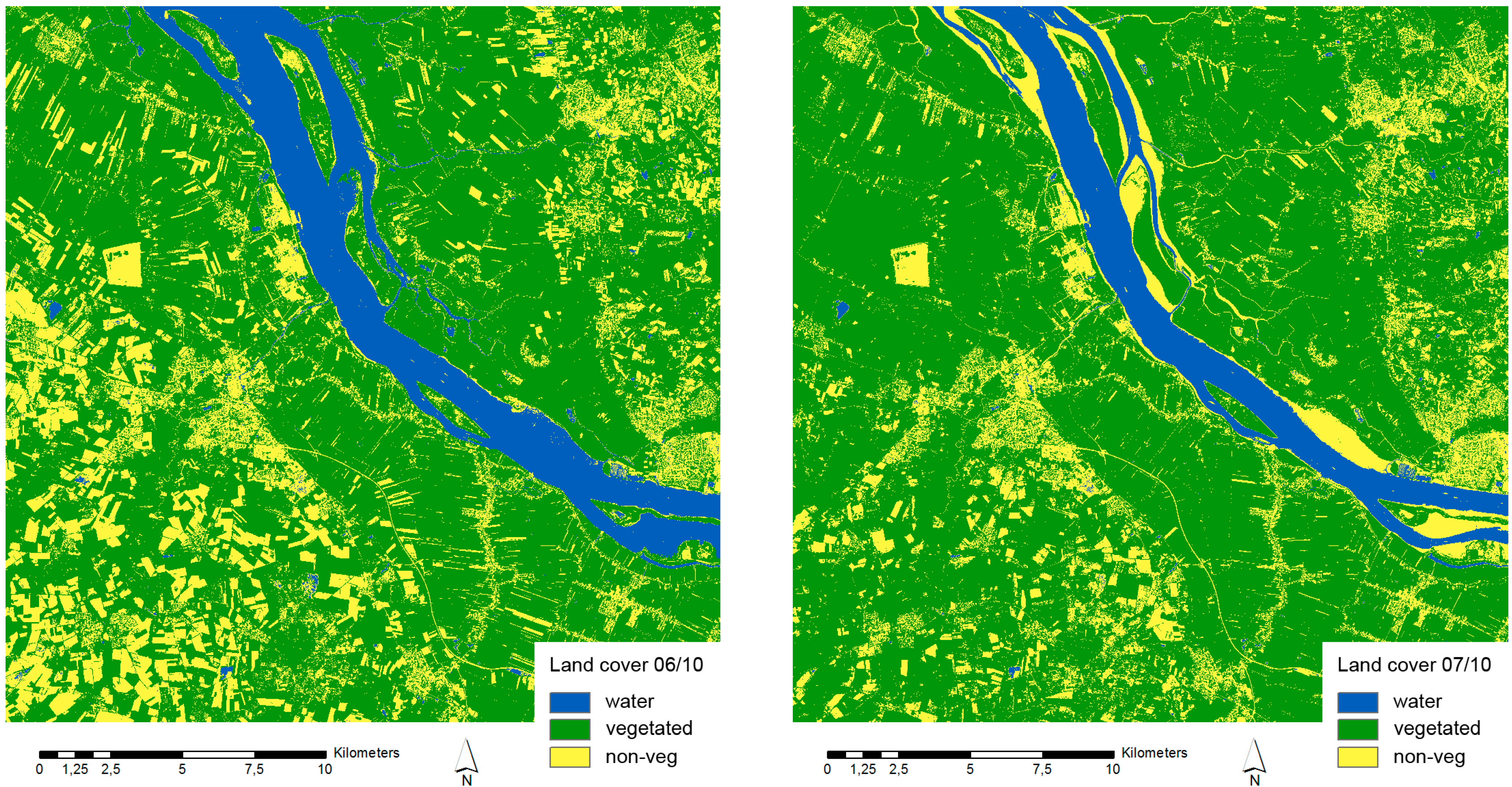
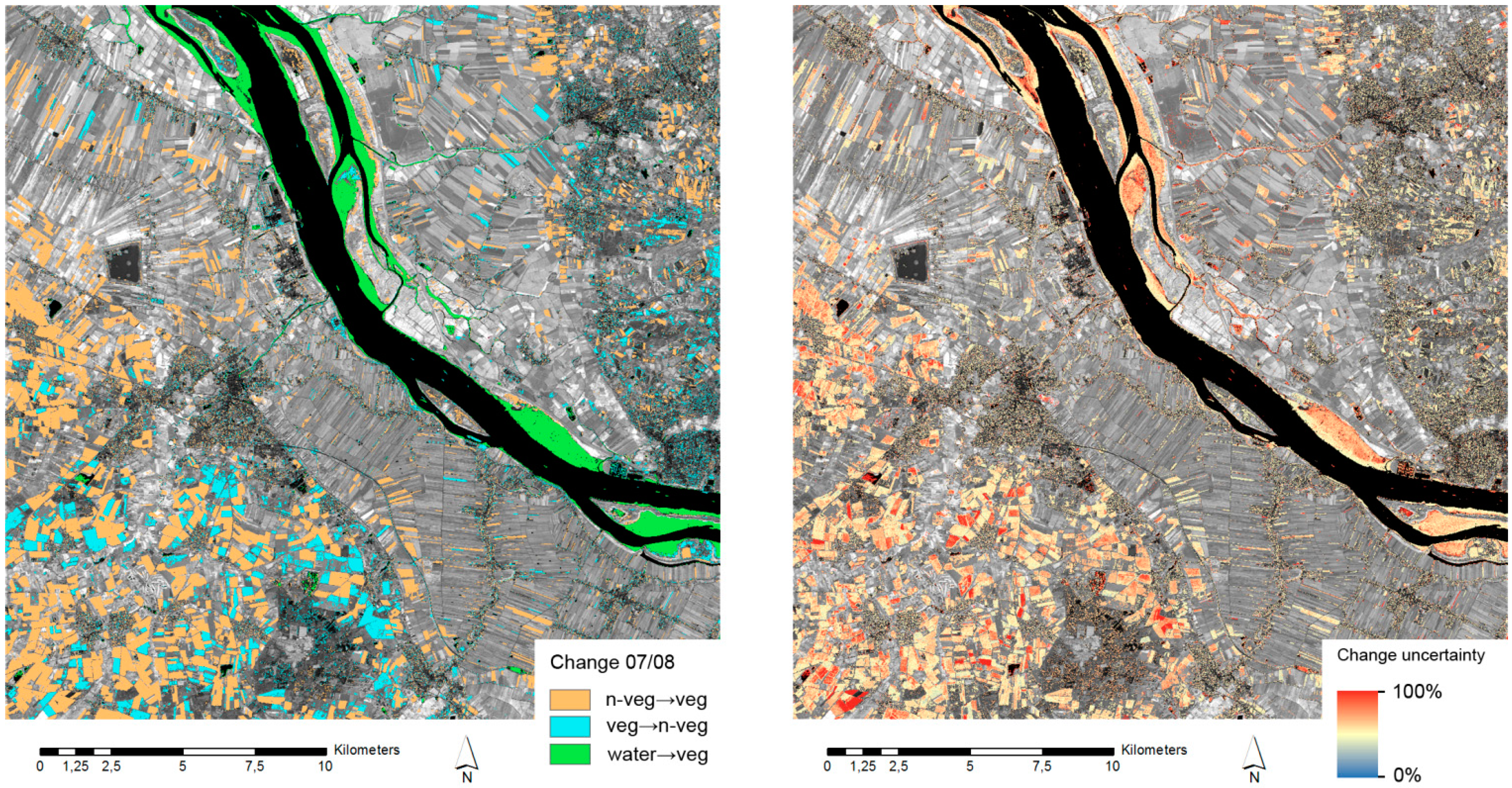
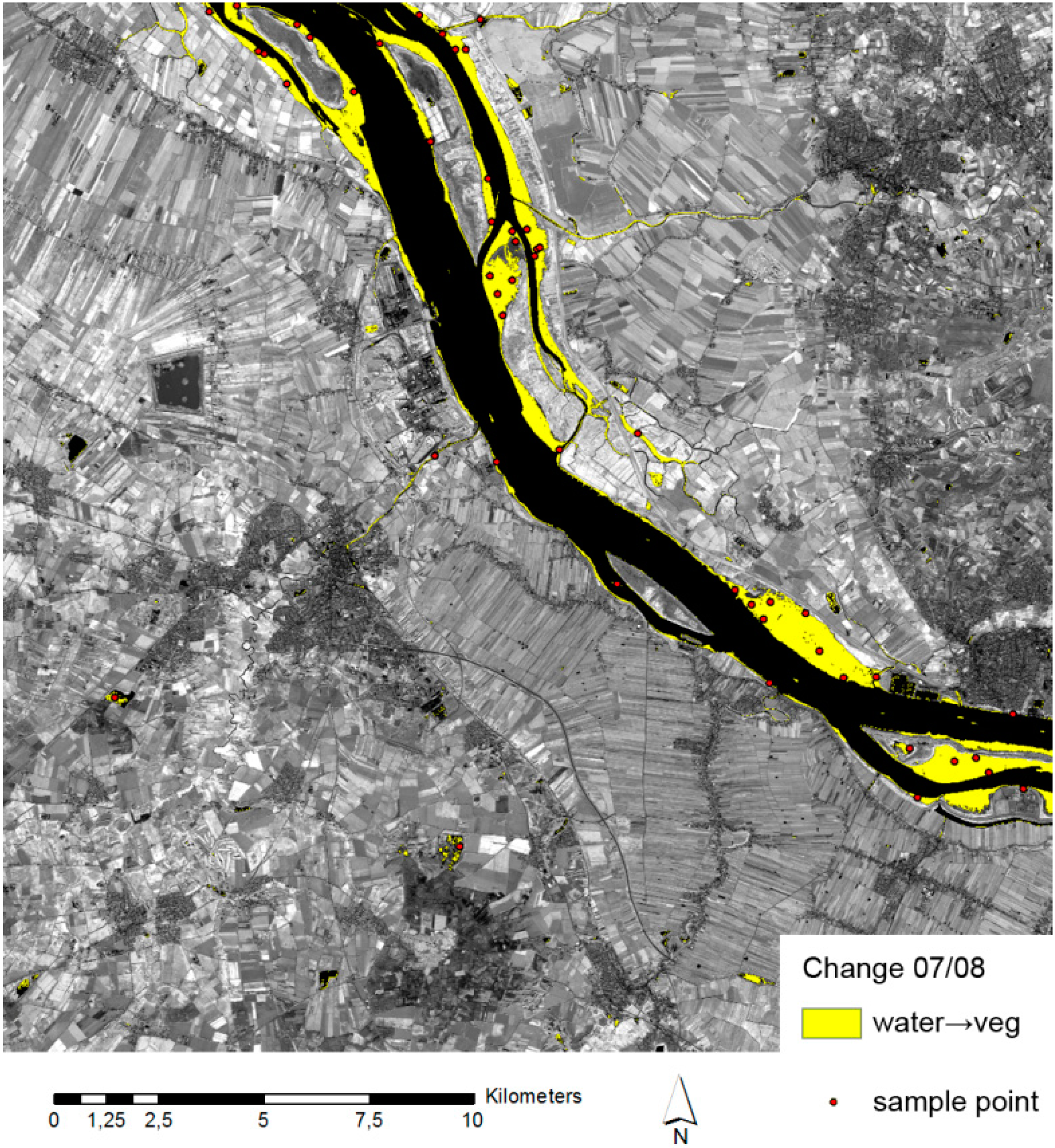
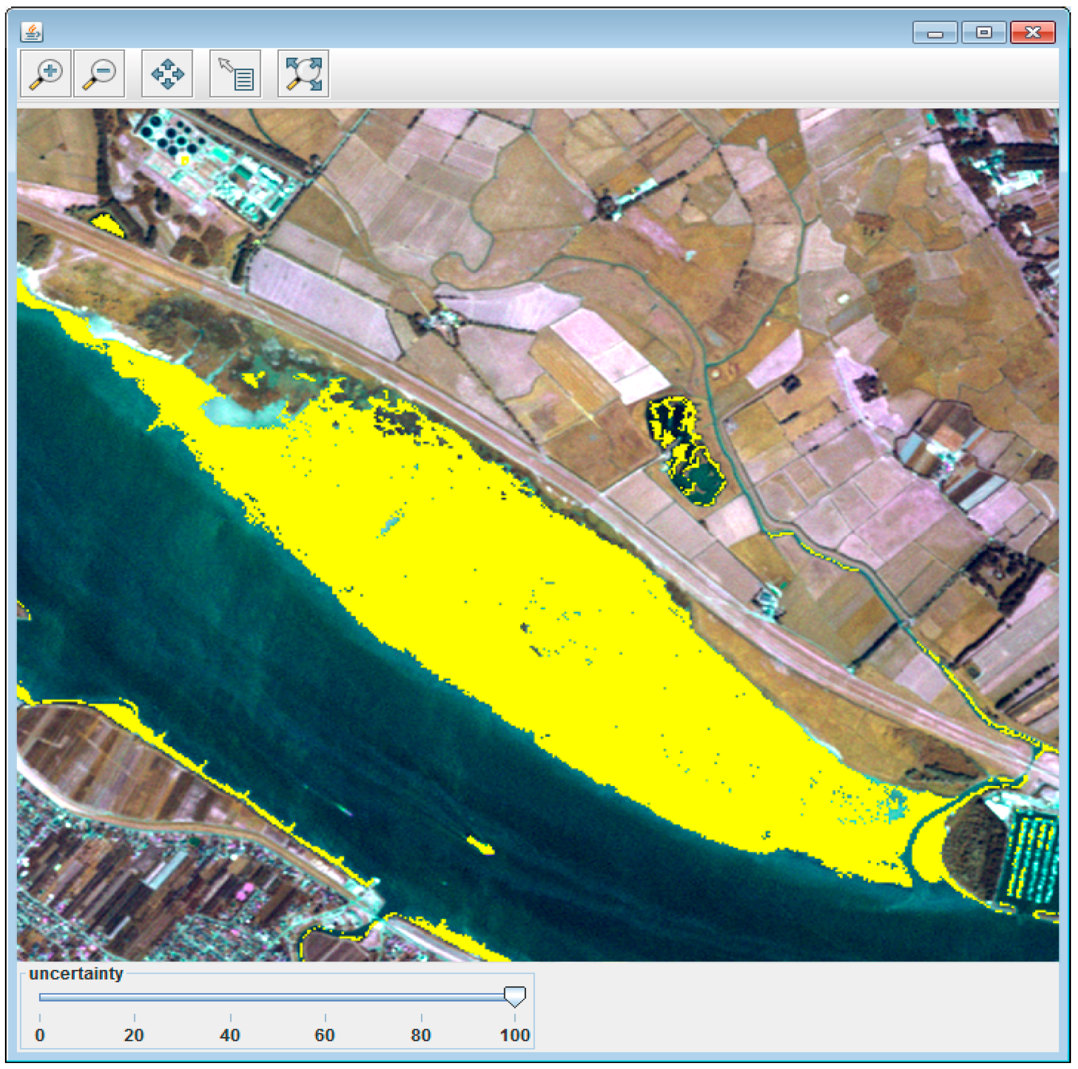
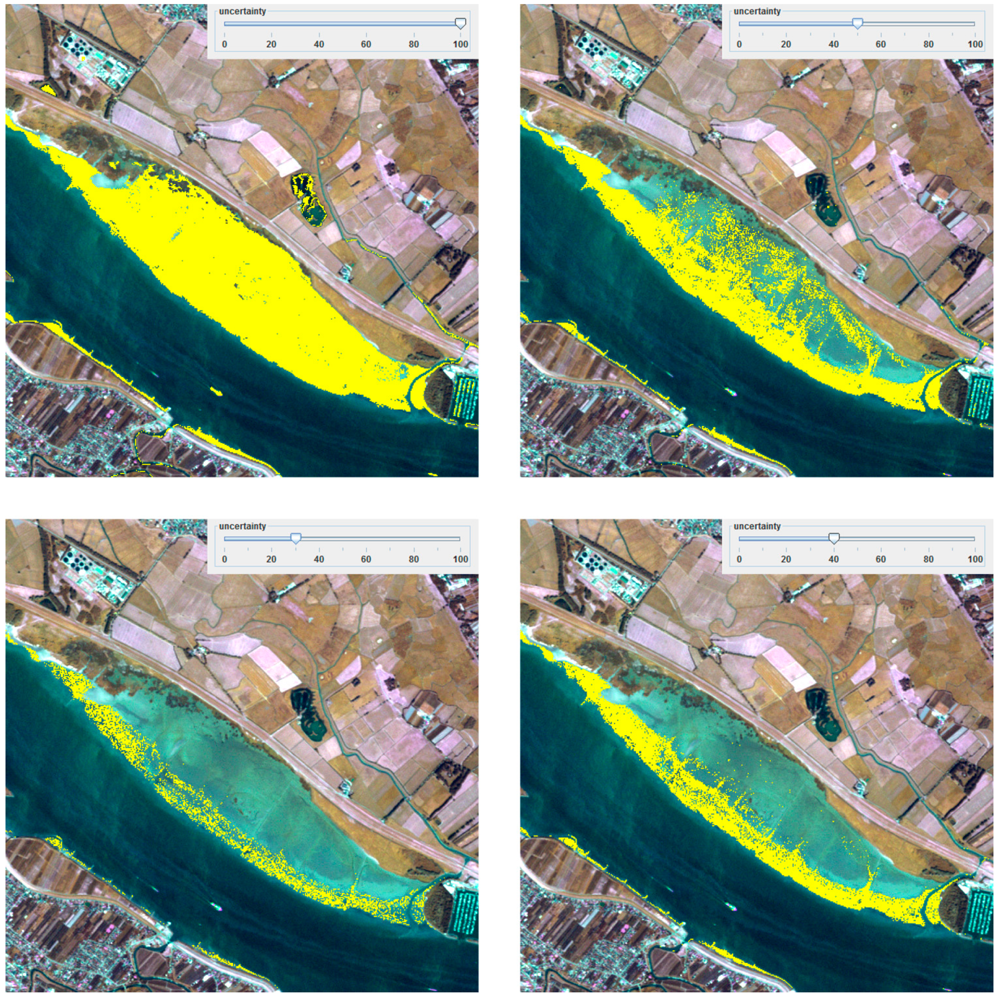
The third potential benefit of using change uncertainty lies in the reduction of falsely detected change. The basic idea is to use high uncertainty as an indicator for erroneous change so that filtering by uncertainty can improve the results. In the workflow presented in Figure 5, the user imports the result from post-classification change detection and the related uncertainty. The next step is to apply filtering so that only changes of a certain type remain. The reason is that it is more likely to find a suitable threshold for a single change type than for changes pertaining to all types. This subset of changes is now visualized along with the connected uncertainty. The initial hypothesis is that this is the optimal change set (in terms of correctness). Now, the user can apply a filter so that only changes with uncertainty less than a certain threshold (e.g., <80%) remain (which can be seen as a revised hypothesis). While changing the filter threshold the user gets immediate visual feedback to help him or her judge if the result has improved or not. When the user is satisfied with the result it can be exported as the final result.

Figure 5. Workflow: Filtering change by uncertainty to reduce false-positive change.

Figure 5. Workflow: Filtering change by uncertainty to reduce false-positive change.

4. Case Study

The following case study serves as proof-of-concept and highlights potential benefits and limitations of the approach for uncertainty-aware change analysis we present here. We created a change scenario based on two satellite scenes from an area in the vicinity of the Elbe River, northwest of Hamburg, Germany. The imagery was taken in 2010, on 5 June and on 16 July, by RapidEye, a satellite system that provides imagery with a geometric resolution of 5 m (pan-sharpened) and a temporal frequency of up to one image every 24 hours under ideal circumstances (http://www.blackbridge.com/rapideye/). The sensor covers five spectral channels, including the so-called “Red Edge” channel between red and near-infrared, giving the sensor potential advantages for vegetation mapping compared to other optical sensors [21]. The imagery we used here was radiometrically corrected and orthorectified (RapidEye Ortho-Level 3A). It was acquired via RapidEye Science Archive (RESA), which provides imagery free of cost for scientific use (http://resa.blackbridge.com/).

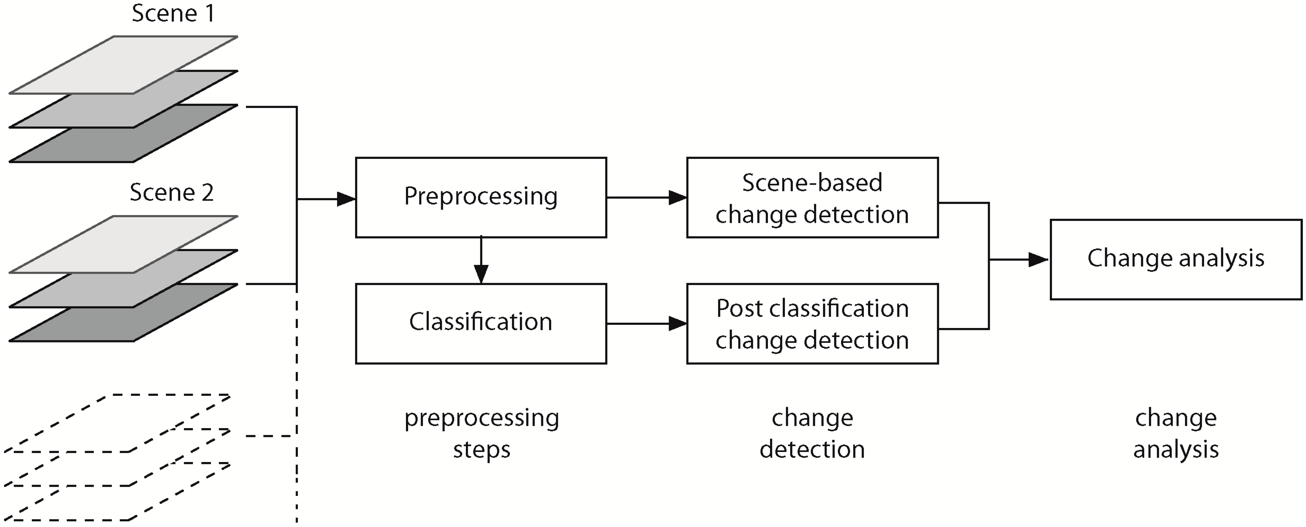
4.1. Change Detection

The area covered by the satellite imagery is a 25 km × 25 km rural agricultural area between Stade and Pinneberg in the vicinity of the Elbe River. Since the images were taken in summer and there were just six weeks between their acquisition we expected that most changes would be related to vegetation and water bodies (due to vegetation growth/harvesting and tidal changes). Therefore, we classified the two scenes separately using ISODATA unsupervised classification with eight classes, and aggregated them in both datasets yielding three classes: “water”, “vegetated area” (i.e., vegetated arable land, meadows, forest, etc.), and “non-vegetated area” (settlements, roads, non-vegetated arable land, etc.). For both scenes most of the land cover is vegetated area, mainly consisting of agricultural crops, meadows, and forests (Figure 6). Non-vegetated area is comprised of bare soil or settlements and roads, but also riverbanks. Most of the area classified as water belongs to the river—a minor part consists of a few small water bodies.

Figure 6. The two classified datasets from RapidEye imagery we used in this case study.

Figure 6. The two classified datasets from RapidEye imagery we used in this case study.

From the aggregated dataset with the three classes described above, we created spectral signatures and rerun the classification using the Maximum Likelihood algorithm to get additional information about the membership values of each pixel. By intersecting the two classified datasets we created a change dataset containing changed areas and their type (Figure 7). On the basis of the class membership values we computed the change uncertainty measure (refer to Section 2). We removed a no-data area in the southeastern corner of the scene and filtered out all changes that occurred in areas smaller than the minimum mapping unit of 1000 m².

Figure 7. Change dataset (left) and related uncertainty (right).

Figure 7. Change dataset (left) and related uncertainty (right).

4.2. Change Analysis

When analyzing the result, the first observation is that 22% of the study area was detected as having changed. Most changes belong to the type “non-vegetated to vegetated” (58% of the changed area), followed by “vegetated to non-vegetated” (28.5%), and “water to non-vegetated” (13%). There was also a very small amount of change from water to vegetated area (about 0.5%) that we did not consider in this analysis. Generally, the detected change types and their resulting area proportions seem plausible considering the two scenes are from June and July, when vegetation growth and harvesting of some crop types is common and therefore may explain most of the detected change.

In order to assess the accuracy of the detected change we conducted a visual assessment with stratified random point sampling over the whole area. We determined the number of points after Tortura’s method of approximation [22]. With an estimated average accuracy of 70% and an error tolerance of 5%, we obtained a required sample size of 323 points. We focused on false positive changes, i.e., changes that have been falsely detected, since they are a common challenge in change analysis (see Section 1). Thus, we only assessed the areas detected as changes and not the no-change areas (false-negatives). Reference data from a different source was not available for the exact two dates so we visually examined each of the points based on the available imagery and estimated the correctness of the change in each position. Consequently, since the assessment conducted here does not rely on independent data, it does not fulfill the requirements of a statistically sound accuracy assessment. However, for the purpose here we see it as sufficient in order to get an impression about the quality of the change set. Table 1 shows the change types, their proportions of the overall area, and their corresponding number of sample points. The last two columns contain the result from the visual assessment.

Table 1. Stratified point sampling and results of the visual assessment of change correctness.

Change Type	Proportion of Overall Area	Number of Sample Points	CorrectChange	Erroneous Change
All	100%	323	-	-
No change	77.7%	251	-	-
Water to non-vegetated	2.9%	9	66.7%	33.3%
Vegetated to non-vegetated	6.3%	21	80.9%	19.1%
Non-vegetated to vegetated	12.9%	42	85.7%	14.3%

Table 1. Stratified point sampling and results of the visual assessment of change correctness.

Change Type	Proportion of Overall Area	Number of Sample Points	CorrectChange	Erroneous Change
All	100%	323	-	-
No change	77.7%	251	-	-
Water to non-vegetated	2.9%	9	66.7%	33.3%
Vegetated to non-vegetated	6.3%	21	80.9%	19.1%
Non-vegetated to vegetated	12.9%	42	85.7%	14.3%

Figure 8. Change uncertainty for “water to non-vegetated area”.

Figure 8. Change uncertainty for “water to non-vegetated area”.

In the following we focused on the change type “water to non-vegetated area” because it showed the highest amount of erroneous change (33.3%). The high error rate is explainable by the uncertainty in separating water bodies from bare areas. The changes from water to non-vegetated areas are due to the different water levels of the river at the two dates. Regarding change uncertainty, the first observation was that all changes of this type that did not occur directly along the bank of the river were highly uncertain. Some small areas of this nature were detected. This corresponds to the assumption that changes from water to non-vegetated areas would only occur along the riverbanks. Small water bodies could potentially dry out in summer, but since this is unlikely in such a short period of time (at least for the area under research) we hypothesize that these small area changes were caused by misclassification. A second observation is that most areas situated directly at the edge of the water seem to be homogeneously certain and become more heterogeneous the further away from the water’s edge they are. Figure 8 shows an exemplary change area at the eastern part of the river. The distribution of uncertainty seems plausible, because directly at the river bed the change is more likely to have happened than when we move further away from the water’s edge. It is obvious that the boundary between the riverbed (belonging to the class “water”) and mud flats on the banks (belonging to the class “non-vegetated areas”) plays an important role for this change type and is highly uncertain at the same time.

For a closer look at the changes from water to vegetated areas we generated 41 additional random sample points over the area covered by this change type to attain 50 random points (Figure 9), which follows the rule of thumb suggested by Congalton and Green [23]. Again, we conducted a visual assessment without independent reference data. The result was that the detected changes at 72% of the points were correct, while 28% were incorrect due to misclassification. For most applications this level of accuracy does not seem acceptable and the change dataset would have to be improved. In the following, we would like to demonstrate how information on change uncertainty can help increase the accuracy of the change dataset.

Figure 9. Sample points (red) in the area of change from water to non-vegetated area (yellow).

Figure 9. Sample points (red) in the area of change from water to non-vegetated area (yellow).

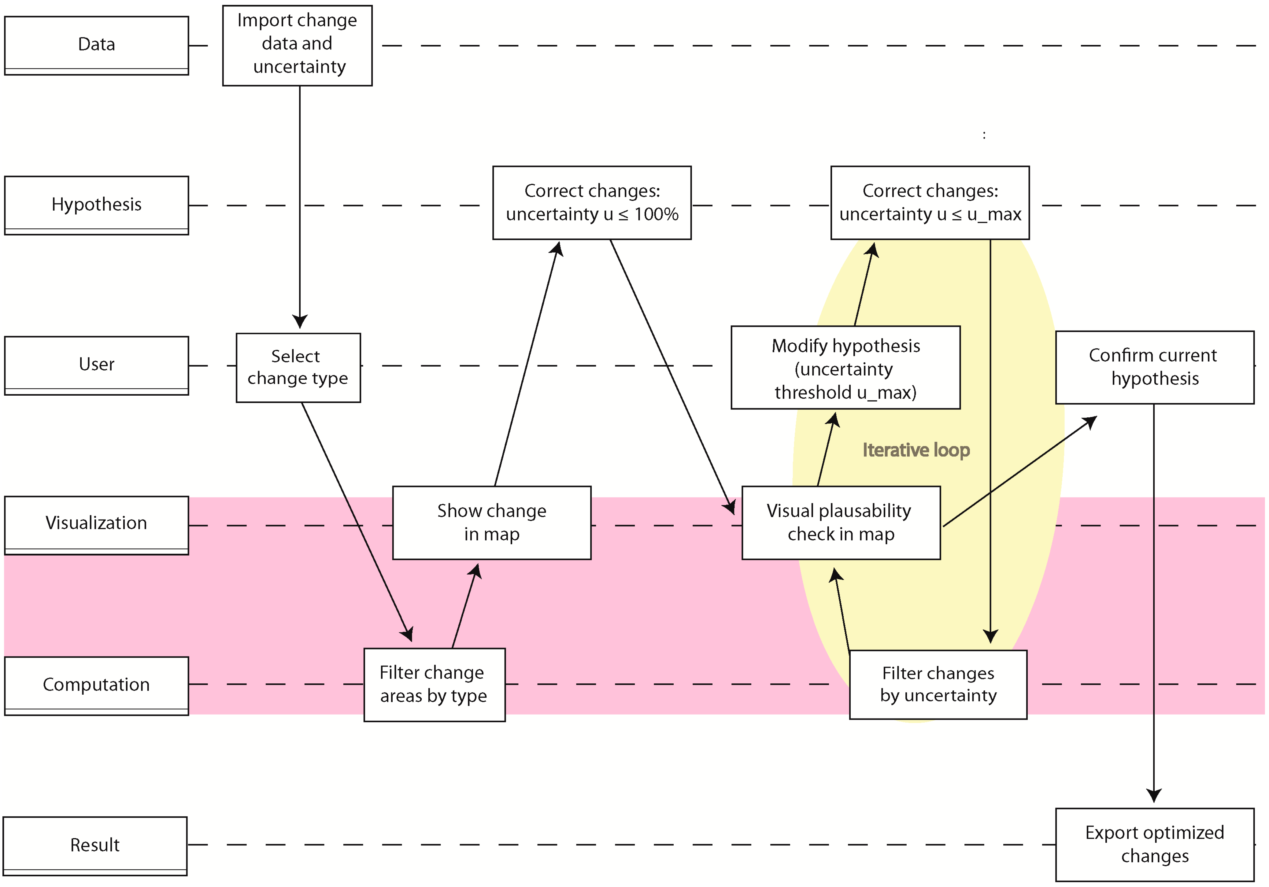
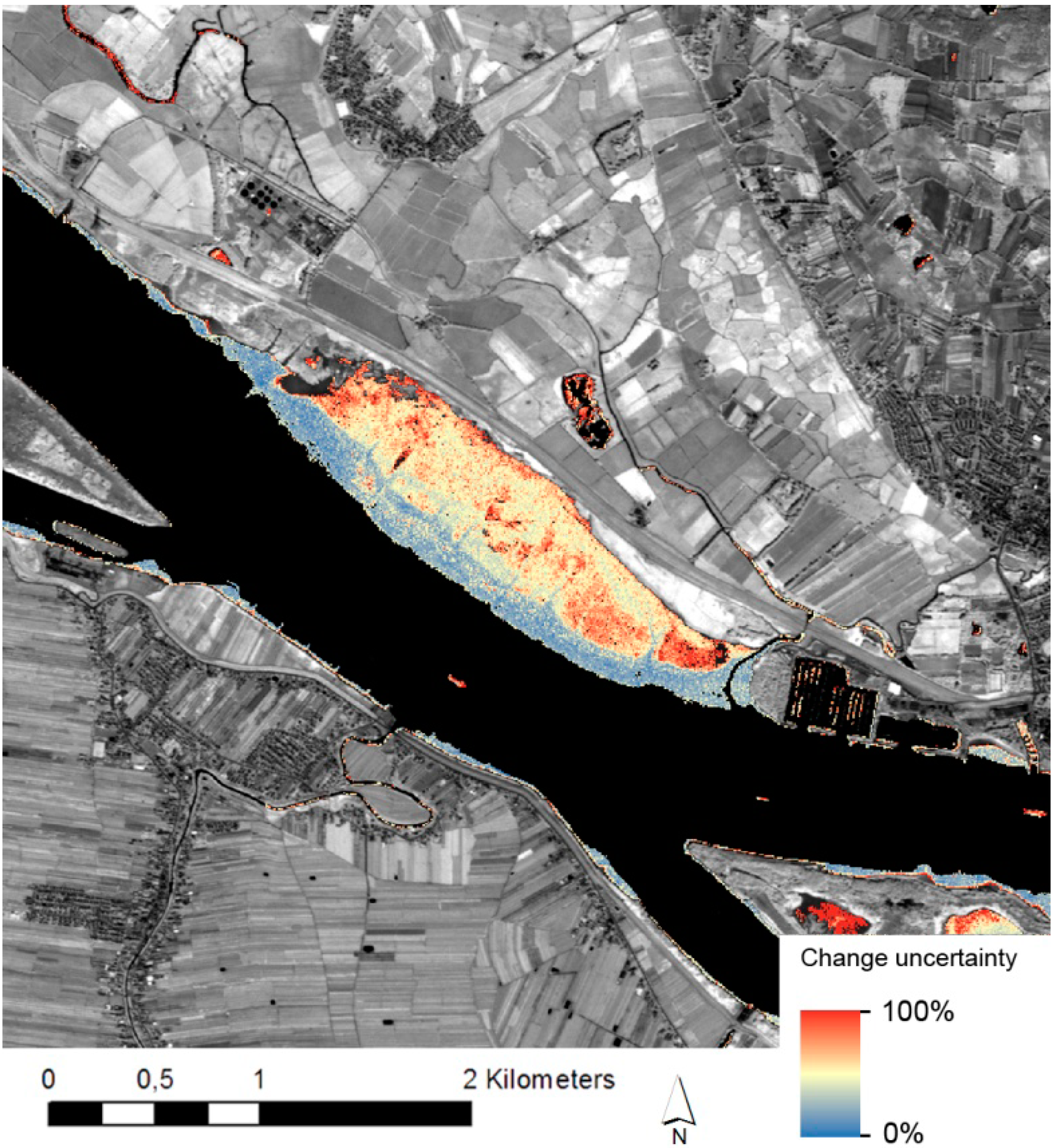
4.3. Reduce False-Positive Change

In Section 3 we hypothesized that the accuracy of detected change could be increased if we filter out uncertain change by applying a suitable threshold. We tested this hypothesis using our change scenario. For this, we utilized a simple prototype including a map client and a slider to filter change by uncertainty (Figure 10). The prototype is written in Java and is based on the geotools map client (http://www.geotools.org/) that provides standard map functionality (pan, zoom, etc.) under a free and open source license. The RS imagery is shown in the background and yellow pixels on the map represent changes. Change uncertainty is visualized using a color scheme from blue (0% uncertainty) to yellow (50%) to red (100%). The slider at the bottom of the window can be used to interactively filter the changes by uncertainty, starting with an initial threshold of 100% (meaning that no changes are filtered out).

Figure 10. Software prototype for iterative filtering by uncertainty.

Figure 10. Software prototype for iterative filtering by uncertainty.

In order to show how erroneous change can be filtered out by thresholding we chose an area of 5 km × 5 km with a large zone of change from water to non-vegetated area (Figure 11). To get started we lowered the threshold so that changed pixels with an uncertainty of more than 50% were filtered out. A visual check showed that this removed a number of questionable areas of change, but not all of them. After modifying the threshold several times and visually checking the outcome, we found that setting the uncertainty threshold to 40% filtered out most of the outliers we had identified on the map, clearly improving the result compared to the initial state. While the threshold was only determined for the small area presented here, we were interested to see if it would work for the whole scene. After taking a closer look at our sample points, it was revealed that all 17 misclassified points were filtered out, i.e., all erroneous change could be eliminated through simple thresholding. Furthermore, only one point with a correct change was (falsely) removed. This shows that a threshold chosen for a local area can work for a larger area such as a whole satellite scene. But it is likely that this does not hold true with scenes that show greater spectral variation as those we used here.

4.4. Discussion

The case study presented here highlighted the potential of uncertainty-aware change analysis using a GVA approach. First, it could be shown that better-informed change analysis is possible and that uncertainty can provide valuable information during the interpretation of detected change. Apart from this, as shown in the case study, uncertainty can serve as an indicator for erroneous change and can be used for filtering. It became clear that it is not a fully reliable indicator, but that it can serve as a criterion when deciding whether a change is correctly detected or not. Further criteria should be taken into account to validate detected change, e.g., the size or spectral signature of a changed area. It became clear that a suitable threshold can be determined locally, e.g., for a single area of change, but that one overall threshold for a whole scene (although it is only for one change type) often does not seem realistic, depending on the change type and the variability in the imagery. One downside of this concept that we mentioned is that by including uncertainty into the analysis and thus adding another data dimension, change analysis becomes more complex. This stresses the importance of minimizing the complexity, for instance by keeping the visual load for the user low.

Figure 11. Iterative filtering of change by 100% (upper left), 50% (upper right), 30% (lower left), and 40% (lower right) uncertainty.

Figure 11. Iterative filtering of change by 100% (upper left), 50% (upper right), 30% (lower left), and 40% (lower right) uncertainty.

In this case study we performed an analysis with the help of a simple prototype. In comparison to standard GIS, it facilitates the straightforward modification of the filter threshold and provides immediate feedback on the map. The simple tool we used here makes iterative analysis more fluent and more intuitive—however, this assumption has not yet been assessed in user studies. We are convinced that with more sophisticated workflows, e.g., when more information about a change is visualized (for example, area, spectral signature, and uncertainty), the advantages compared to common GIS analysis will become more apparent.

5. Conclusions

In this article we presented a concept to enhance the analysis of change derived from remote sensing (RS) data. The idea was to incorporate information about uncertainty concerning detected changes into the analysis. We suggested a geovisual analytics (GVA) approach that combines manual and automated analysis with the help of visual interfaces. This contributes to a better integration of change detection and analysis as well as to an enhanced visual communication of uncertainty during the analysis. We defined a measure for change uncertainty and identified potential applications of the concept. In a case study we used a simple software prototype that showed changes on a map and provided filtering by uncertainty. The study included a bi-temporal change scenario with RS data in the vicinity of the Elbe River near Hamburg, Germany, and showed how false positive changes could be successfully filtered out by the use of uncertainty thresholding. We pointed out that generally, uncertainty can be an indicator for erroneous change, however, it has limitations since the critical level of uncertainty (for the distinction between correct and erroneous change) may vary within a dataset. Thus, we recommended the use of other additional indicators to help decide whether changes are correct, e.g., the area of a change or its spectral signature.

All in all, it was shown that tools implementing the concept have the potential to counter challenges in change analysis such as the high amount of false positive changes. At the same time, analysis naturally becomes more complex since uncertainty adds another dimension of data that has to be taken into account. This fact stresses the importance of well-crafted visual interfaces and interaction functionality to minimize user burden. User studies will be necessary to evaluate if analysts can use uncertainty information when it is visually depicted and how they cope with the complexity and visual load that is added when incorporating uncertainty.

The case study we presented here involved a bi-temporal analysis of change. But the concept allows analysis of more than two RS datasets at a time and we hypothesize that this is one of the strengths of the approach. This will have to be tested in future studies involving more than two RS scenes.

The software prototype we used in the case study shall serve as a starting point for more complex change analysis tools of this kind. Thus, an important part of future work will be the derivation of guidelines and recommendations to support the development of change analysis tools based on this concept. These should include recommended techniques for uncertainty visualization and user interaction. All in all, we see the support for GVA tool development as a crucial step to get closer to the goal of establishing tools for uncertainty-aware analysis of change that can be used in practice.

References

1. Zhang, J.; Goodchild, M.F. Uncertainty in Geographical Information; Taylor & Francis: London, UK, 2002. [Google Scholar]
2. Pontius, R.G., Jr.; Lippitt, C.D. Can error explain map differences over time? Cartogr. Geogr. Inf. Sci. 2008, 33, 159–171. [Google Scholar] [CrossRef]
3. Coppin, P.; Jonckheere, I.; Nackaerts, K.; Muys, B. Digital change detection methods in ecosystem monitoring: A review. Int. J. Remote Sens. 2004, 25, 1565–1596. [Google Scholar] [CrossRef]
4. De Chiara, D. From GeoVisualization to Visual-Analytics: Methodologies and Techniques for Human-Information Discourse. Ph.D. Thesis, University of Salerno, Salerno, Italy, February 2012. [Google Scholar]
5. Tomaszewski, B.M.; Robinson, A.C.; Weaver, C.; Stryker, M.; MacEachren, A.M. Geovisual analytics and crisis management. In Proceedings of the 4th International Information Systems for Crisis Response and Management (ISCRAM) Conference, Delft, The Netherlands, 13–16 May 2007.
6. Schiewe, J. Geovisualisation and geovisual analytics: The interdisciplinary perspective on cartography. In Proceedings of 26th International Cartographic Conference ICC 2013, Dresden, Germany, 25–30 August 2013; pp. 122–126.
7. Wang, T.D.; Wongsuphasawat, K.; Plaisant, C.; Shneiderman, B. Extracting insights from electronic health records: Case studies, a visual analytics process model, and design recommendations. J. Med. Syst. 2011, 35, 1135–1152. [Google Scholar] [CrossRef]
8. Schreck, T.; Tekušová, T.; Kohlhammer, J.; Fellner, D. Trajectory-based visual analysis of large financial time series data. ACM SIGKDD Explor. Newsl. 2007, 9, 30–37. [Google Scholar] [CrossRef]
9. Lucieer, A. Uncertainties in Segmentation and Their Visualization. Ph.D. Thesis, Utrecht University, Enschede, The Netherlands, 2004. [Google Scholar]
10. Ahlqvist, O. Extending post-classification change detection using semantic similarity metrics to overcome class heterogeneity: A study of 1992 and 2001 U.S. National Land Cover Database changes. Remote Sens. Environ. 2008, 112, 1226–1241. [Google Scholar] [CrossRef]
11. Bastin, L.; Fisher, P.; Wood, J. Visualizing uncertainty in multi-spectral remotely sensed imagery. Comput. Geosci. 2002, 28, 337–350. [Google Scholar] [CrossRef]
12. Zurita-Milla, R.; Blok, C.; Retsios, V. Geovisual analytics of Satellite Image Time Series. In Proceedings of the 2012 International Congress on Environmental Modelling and Software, Leipzig, Germany, 1–5 July 2012; Seppelt, R., Voinov, A.A., Lange, S., Bankamp, D., Eds.; International Environmental Modelling and Software Society (iEMSs): Leipzig, Germany, 2012; pp. 1431–1438. [Google Scholar]
13. Green, K. Change matters. Photogramm. Eng. Remote Sens. 2011, 77, 305–309. [Google Scholar] [CrossRef]
14. Hoeber, O.; Wilson, G.; Harding, S.; Enguehard, R.; Devillers, R. Visually representing geo-temporal differences. In Proceedings of the IEEE Conference on Visual Analytics Science and Technology 2010, Salt Lake City, USA, 25–26 October 2010; MacEachren, A., Miksch, S., Eds.; IEEE Press: New York, NY, USA, 2010; pp. 229–230. [Google Scholar]
15. Foody, G.M.; Atkinson, P.M. (Eds.) Uncertainty in Remote Sensing and GIS; Wiley: Hoboken, NJ, USA, 2002. [CrossRef]
16. Shi, W.; Fisher, P.F.; Goodchild, M.F. (Eds.) Spatial Data Quality; Taylor & Francis: New York, NY, USA, 2002.
17. Fisher, P.; Arnot, C.; Wadsworth, R.; Wellens, J. Detecting change in vague interpretations of landscapes. Ecol. Inform. 2006, 1, 163–178. [Google Scholar] [CrossRef]
18. Brown, K.M.; Foody, G.M.; Atkinson, P.M. Deriving thematic uncertainty measures in remote sensing using classification outputs. In Proceedings of the 7th International Symposium on Spatial Accuracy Assessment in Natural Resources and Environmental Sciences, Lisbon, Portugal, 5–7 July 2006; Caetano, M., Painho, M., Eds.; Instituto Geográfico Português: Lisbon, Portugal, 2006. [Google Scholar]
19. Lowry, J.H.; Ramsey, R.D.; Langs Stoner, L.; Kirby, J.; Schulz, K. An ecological framework for evaluating map errors using fuzzy sets. Photogramm. Eng. Remote Sens. 2008, 74, 1509–1519. [Google Scholar] [CrossRef]
20. Burnicki, A.C. Modeling the probability of misclassification in a map of land cover change. Photogramm. Eng. Remote Sens. 2011, 77, 39–49. [Google Scholar]
21. Schuster, C.; Förster, M.; Kleinschmit, B. Testing the red edge channel for improving land-use classifications based on high-resolution multi-spectral satellite data. Int. J. Remote Sens. 2012, 33, 5583–5599. [Google Scholar] [CrossRef]
22. Khorram, S. Accuracy Assessment of Remote Sensing-Derived Change Detection; American Society for Photogrammetry and Remote Sensing: Bethesda, MD, USA, 1999. [Google Scholar]
23. Congalton, R.G.; Green, K. Assessing the Accuracy of Remotely Sensed Data: Principles and Practices, 2nd ed.; CRC Press/Taylor & Francis: Boca Raton, FL, USA, 2009. [Google Scholar]