Dasymetric Mapping and Spatial Modeling of Mosquito Vector Exposure, Chesapeake, Virginia, USA

Abstract

Complex biophysical, social, and human behavioral factors influence population vulnerability to vector-borne diseases. Spatially and temporally dynamic environmental and anthropogenic patterns require sophisticated mapping and modeling techniques. While many studies use environmental variables to predict risk, human population vulnerability has been a challenge to incorporate into spatial risk models. This study demonstrates and applies dasymetric mapping techniques to map spatial patterns of vulnerable human populations and characterize potential exposure to mosquito vectors of West Nile Virus across Chesapeake, Virginia. Mosquito vector abundance is quantified and combined with a population vulnerability index to evaluate exposure of human populations to mosquitoes. Spatial modeling is shown to capture the intersection of environmental factors that produce spatial hotspots in mosquito vector abundance, which in turn poses differential risks over time to humans. Such approaches can help design overall mosquito pest management and identify high-risk areas in advance of extreme weather.

1. Introduction

The spread of vectors and growing number of vector-borne diseases pose a major threat to human health. In order to prevent the spread of disease, it is advantageous to predict the risk of disease transmission, both spatially and temporally. Geospatial technologies are commonly used to evaluate patterns of vector or human case distributions, as well as estimate the risk of disease transmission based on entomological, epidemiological, and environmental factors [1]. One limitation is that prediction systems are often static and only predict risk at one particular time and place. This study has addressed this shortcoming by predicting the risk of disease transmission from mosquitoes across Chesapeake, Virginia, for the summer of 2003, following a broad scale field surveillance campaign by this city’s Mosquito Control Commission. In a situation where a disease or hazard is rare (and control-case studies or cohort studies are impractical), analyzing trends in threats and coexistence of risk factors with disease are fruitful approaches [2]. Using GIS techniques, spatial analyses were conducted in this study to track the trends in competent vector species abundance and identify coincident population most susceptible to mosquito-borne diseases and estimate relative risk of disease transmission to humans.

Predictions of human sensitivity and potential disease transmission have been recommended to incorporate vector abundance and the immune status of the host population [3]. Such epidemiological evidence is also translated into surveillance and control of vector species by local public health agencies. In addition, the risk of exposure to mosquito-borne disease vectors may be estimated using mosquito abundance values and the broad physiological factors of human vulnerability to disease infection. Mosquito abundance values for this project were derived from a previously published study measuring the abundance of competent mosquito vector species Culiseta melanura as well as the combined abundance of Aedes vexans and Psorophora columbiae [4,5]. A. vexans and P. columbiae share a habitat preference for ephemeral pools and therefore are referred to as the “ephemeral species” throughout this paper. C. melanura is an important species in this region because it is the primary enzootic vector of Eastern Equine Encephalitis (EEE) and is also a potential vector of West Nile Virus (WNV). A. vexans is also another important potential epizootic vector for WNV. While several studies use vector and environmental variables to estimate risk, many studies do not take into account human vulnerability to these diseases or the temporal and spatial variability of vector abundance or human demographics and activity spaces.

A primary objective of this study is to estimate human exposure to mosquito vector species capable of disease transmission and human infection across a landscape. The City of Chesapeake, Virginia, offers this setting with a populous urban to rural gradient and low topographic coastal location adjoining extensive mosquito habitats that are exceedingly productive in the humid, subtropical summer climate, including abundance of ephemeral pools, agricultural ditches, and container breeding sites in urbanized areas. The second objective is to map the vulnerable human population in a manner that depicts the most accurate distribution of the population and facilitates assessing potential vector exposure risk. Using monthly mosquito abundance values and human population vulnerability data, a monthly risk index is calculated which estimates the exposure to mosquito vector species. These objectives underscore the overall goal of this study, to improve prediction of the risk of exposure to mosquitoes across Chesapeake, Virginia, during the peak mosquito breeding summer months of June to August. In addition, an achievable and practical result of this analysis includes a spatial risk model that can be adapted to other regions to identify vector exposure for surveillance and control, demonstrating geographic-targeting and more sophisticated, micro-level control measures [6].

A growing number of studies have predicted disease risk using geospatial methods (remote sensing, spatial analysis, geovisualization, and other methods applying and integrating Geographic Information Systems (GIS)). Statistical approaches to predicting outbreaks of West Nile Virus (WNV) using land cover and environmental factors, for instance, have been developed for Indianapolis, Indiana [7]. A spatial-temporal model was created that predicted disease risk from 2002 through 2007. This study found that the highest clusters of WNV outbreaks were located in agriculture and grassland areas. Such cover types exhibited a relatively high moisture content and provided favorable habitats for mosquito breeding. Discriminant analysis was used to find the relationship between environmental variables and disease. The results indicated that certain variables had a high impact on WNV dissemination. Wetland size, agriculture area percentage, and stream length were all positively correlated with WNV outbreaks. WNV infection potential has also been studied using a wide sample of dead birds and human population data with cluster analysis to infer potential disease infection hotspots [8]. In another empirical study combining LandScan gridded population data and Aedes aegypti mosquito species distribution maps, correlation and monte carlo simulation analyses related human mobility, vector abundance, and disease transmission [9]. Indeed, GIS and remote sensing techniques have been used to assess mosquito-borne disease risk widely, even globally as in the case for malaria risk [10]. NASA scientists at the Goddard Space Flight Center’s Healthy Planet program developed a malaria transmission model that incorporates parasites, hosts, vectors, human factors, and environmental factors. They also developed a risk model that predicts transmission intensity using meteorological data. Remotely sensed imagery was used to identify potential breeding sites of mosquito vectors in order to better focus mosquito control applications. Similar work pioneered by Beck et al. investigated satellite remote sensing and GIS techniques to identify the risk of malaria transmission in Chiapas, Mexico, for identifying villages with high vector-human contact risk [11].

Although GIS has been widely used for disease risk estimation, one limitation is the dearth of human health data incorporated into risk models. However, vulnerability is an important factor that can guide estimations of the risk of disease infection. Factors such as age, immune suppression, activity space and behavior patterns, and genetics influence a human’s risk of infection. The spatial pattern of infectious and susceptible people to vector-borne diseases may be a critical determinant of exposure and disease risk [12]. Using demographic and GIS data, this study estimates the population that is most vulnerable to mosquito-borne exposure across the City of Chesapeake. Initial assessment of vulnerability utilizes mapped U.S. Census block group demographics. Aggregating population density to geographic units such as Census blocks, block groups, or tracts is a common method for creating choroplethic maps of population data. One constraint of these maps is that the reader is left to assume that all areas within a given geographic unit have equal population densities. However, this is usually not the case and presents an impediment to understanding finer scale patterns. If the spatial units are too large, a commonplace occurrence in suburban to rural settings, the data spatial variation tends to be reduced or overgeneralized [13]. Statistical techniques such as dasymetric mapping can be used to show a more accurate distribution of the population by disaggregating spatial data in polygonal areas to a finer unit of analysis using ancillary data to help refine locations of the population [14]. The technique has been succinctly described cartographically, “dasymetric mapping depicts quantitative areal data using boundaries that divide the mapped area into zones of relative homogeneity with the purpose of best portraying the underlying statistical surface” ([15], p. 125). This method of mapping transforms data from the arbitrary or choroplethic zones of data aggregation to a dasymetric map in order to enhance and depict the spatial pattern of human population. The transformation of data from the arbitrary zones of the source data to the meaningful zones incorporates the use of an ancillary data set that is separate from, but related to, the variation in the statistical surface [16].

The most common dasymetric technique is the grid binary method in which ancillary classes are regarded as either populated or unpopulated [15]. This particular study uses the “intelligent” dasymetric mapping (IDM) approach to map human vulnerability [17]. The IDM approach takes data mapped in polygonal “source” zones and a second, categorical grid data set, then redistributes the polygonal population data to a set of target zones formed by the intersection of the source and ancillary grid units. In this project, intelligent dasymetric mapping is used to display the vulnerable population according to land cover classes. The final output is a raster surface, which displays vulnerability per pixel unit. This representation of the population provides a more accurate spatial representation of the vulnerable population throughout Chesapeake as compared to coarser observational units in choroplethic maps.

Tradeoffs in data collection, cartographic output, and spatial data representation must be considered when selecting methods for spatial analysis and map symbolization. Most often, cadastral boundaries or census data polygons are selected by default. There are several reasons why these frequently chosen units are not always the most effective for mapping population data. For instance, this approach may not be appropriate for showing population data over time, as census boundaries may change over each censusing period in tandem with the population settlement pattern and density [18]. Census data also pose a problem because these data often have an uneven spatial distribution. Oftentimes, the cartographer may want to estimate the population within a smaller unit of a census block. Dasymetric maps, on the other hand, can show a population at a much finer scale than a tract, block group or block, such as a grid derived from a satellite image in raster cells. Another issue with census or vector data is that in some parts of the world, these data may not be current or readily available [14]. Satellite imagery is available for all parts of the world and can be used to create dasymetric maps of the population. Although dasymetric techniques are effective for creating thematic maps, the lack of standardization of production methods has reduced the use of dasymetric maps in GIS [15].

Because vector-borne disease incidence is intrinsically dependent on exposure to the disease pathogen and vectors, human vulnerability indices must necessarily derive from overlays with the mosquito abundance values in order to estimate risk. In such an approach, spatial overlay becomes the critical proxy for potential spatial interaction between vectors and humans. The factors affecting disease transmission are temporally dynamic, thus a mosquito vector exposure index is calculated on a monthly basis for June through August of 2003. Predictions were limited to the summer of 2003 due to the ample mosquito trap data available for these months. The selected year also provided an ideal opportunity to analyze a large volume of local mosquito data collected during a relatively wet, increasingly favorable breeding season. Further, the season preceded a landfalling hurricane (Isabel, 17–18 September 2003) whose aftermath elicited widespread aerial adulticide spraying (insecticide for adult mosquitoes.) Hence, the summer of 2003 in Chesapeake provides a rich spatial data set for surveillance of mosquitoes, before subsequently profound changes in mosquito surveillance reduced the volume and spatial extent of mosquito observations (light traps, larval dips, nuisance reports, and landing counts) in the study area. The summer months also represent the prime breeding period for these mosquitoes, as the high temperatures and abundant precipitation create an ideal habitat for mosquito populations to thrive. Six indices are calculated which represent the monthly potential exposure to mosquito vectors from both groups of mosquito species. The exposure risk indices are calculated on a raster grid on a pixel-by pixel basis.

2. Study Area

Chesapeake is an independent city, which comprises 88,000 hectares (340 square miles) of Southeastern Virginia and a population of approximately 220,000 (estimated 2008) during the study. The city is located in the coastal plain of Virginia and contains the northeastern portion of the Great Dismal Swamp (Figure 1). Although it serves as a large reservoir of bird and mosquito vectors, the Great Dismal Swamp was excluded from the study area because there are no permanent residents in the swamp. Nonetheless, mosquito observations are reported from immediate surroundings, and the extensive wetlands and non-tidal creeks, agricultural and stormwater ditches within Chesapeake are conducive to mosquito breeding and therefore an extensive suitable habitat. The proximity of these mosquito habitats to the urbanized areas of Chesapeake allows mosquitoes to easily encounter and potentially transmit diseases to humans. Mosquito abundance was predicted to be high across Chesapeake due to Hurricane Isabel, which made landfall in North Carolina on 18 September 2003 [19]. Chesapeake was also chosen as the study area for its noteworthy mosquito surveillance program. In 2003, the City of Chesapeake Mosquito Control Commission (CMCC) [20] collected mosquitoes using 56 CO₂ baited light traps distributed among 28 permanent sites. Bi-weekly, monthly, and seasonal totals of all species were collected and were made available to the research project. Mosquito captures were collected and counted weekly from April through November of 2003 by a set of staff trained in taxonomy. The mosquito counts were used to predict the mosquito abundance values that are incorporated in the risk model. Focusing on the summer peak breeding months prior to Hurricane Isabel, only the mosquito counts from June through August were used, as these months had sufficient capture data for statistical analysis. In addition, as concerns over potential WNV outbreak evolved, dead birds, cases of Eastern Equine Encephalitis (EEE has historic prevalence in this area), and public mosquito abatement service requests were georeferenced for possible analysis and comparison to mosquito vector trap data and human population exposure.

3. Data and Methodology

3.1. Predicting Population Vulnerability to Disease Risk

To assess the population most susceptible to disease, a choroplethic map of population vulnerability was created. Using 2000 U.S. decennial Census data and a set of augmented GIS point vulnerabilities, the vulnerable population was estimated across Chesapeake. A choroplethic map was created to depict the population mapped according to Census block groups. The vulnerable population data were then partitioned into land use zones using dasymetric mapping techniques.

Census block group statistics provided the initial baseline vulnerable population data. The elderly are at greatest risk of developing severe disease after infection by a mosquito [21]. In addition, children are also at high risk of disease infection owing to their underdeveloped immune systems [22]. To predict the age density, a 2000 decennial Census polygon shapefile was obtained and clipped to the extent of Chesapeake, Virginia. The shapefile included 2004 population estimates per block group. 2004 estimates were used due to the absence of Census data specific to 2003. To tally the elderly and childhood population in our estimates, the sum of population was calculated for persons less than 5 years of age and greater than 50 years of age within each Census block group (Figure 2). Although the typical age for elderly would classify at 65 years or above, there is research supporting the prevalence of persons over 50 to exhibit symptoms, receive hospitalization, and incur a higher case-fatality ratio [23]. The combined total of these age groups per block group is shown in the choroplethic map in Figure 3.

Figure 1. Study area location City of Chesapeake, Virginia, a low-lying coastal plain situated adjacent to the Great Dismal Swamp and extensive estuaries of the Chesapeake Bay. Map shows the Chesapeake Mosquito Control District boroughs superimposed on a Normalized Difference Vegetation Index (NDVI) image from Landsat Thematic Mapper, 29 July 2002. NDVI shows brighter green tones for healthy vegetation.

Figure 1. Study area location City of Chesapeake, Virginia, a low-lying coastal plain situated adjacent to the Great Dismal Swamp and extensive estuaries of the Chesapeake Bay. Map shows the Chesapeake Mosquito Control District boroughs superimposed on a Normalized Difference Vegetation Index (NDVI) image from Landsat Thematic Mapper, 29 July 2002. NDVI shows brighter green tones for healthy vegetation.

Figure 2. Census 2000 population age mapped as choropleths by block groups with point locations of vulnerable populations (hospitals, daycares, schools, etc.) displayed using proportional symbols for discrete population concentrations.

Figure 2. Census 2000 population age mapped as choropleths by block groups with point locations of vulnerable populations (hospitals, daycares, schools, etc.) displayed using proportional symbols for discrete population concentrations.

Figure 3. Vulnerable populations derived for Census block group in persons per hectare (estimated using Equation (1)).

Figure 3. Vulnerable populations derived for Census block group in persons per hectare (estimated using Equation (1)).

Census data are also limiting in that they reflect a “nighttime” population distribution. This cannot account for daytime locations. Urban areas such as Chesapeake are known to experience diurnal surging of population density with workplace and suburban residential commuting. In addition, sites of frequent visitation that are non-domicile are not reflected in the Census, such as hospitals, child care facilities, schools, and outpatient clinics. To account for this discrepancy, points of higher possible vulnerable populations were sought for inclusion in the vulnerable population analysis. These locations are considered particularly important given the large proportion of children and elderly populations at these sites. Hospitals are also considered vulnerable due to the high number of people with compromised immune systems. To complete the second step of vulnerability prediction, vulnerable point facility location data was obtained from the City of Chesapeake Information Technology Department. The data was obtained in the form of a GIS points shapefile in which each feature represents a vulnerable point location (Figure 2). The population of each hospital and elderly care facility were included within the GIS data and counted as permanent residents. The population of Chesapeake General Hospital, for example, was calculated by summing the total number of inpatients and outpatients. School and daycare centers were also included, however, population counts for these facilities were so sparse that additional count inquiry was limited to primary, elementary, and intermediate schools. Determining the population of every daycare was cost-prohibitive across this extensive area having over 250 permitted facilities. Nonetheless, inclusion of site-specific vulnerable populations using these ancillary data and summing with Census data is believed to provide a robust first-order estimate, conservatively estimating the gross vulnerable population and reflecting a slightly higher population that Census nighttime and undercounts would tend to include.

To calculate the final vulnerable population within each block group, the population of each vulnerable point was added to the previously calculated block group vulnerable population based on point-in-polygon overlay. The final output was stored as a polygon shapefile (Equation (1)). In order to reflect the total population in each block group, the vulnerable population was normalized using the following equation and subsequently areally transformed from persons per block group to persons per hectare:

(1)

• Population_n = the normalized vulnerable population, per block group;
• Population_v = the calculated vulnerable population, per block group;
• Population_Total = total population of the block group.

3.2. Dasymetric Mapping of Population Vulnerability

In order to provide a more accurate depiction of how the demographic data is distributed within each block group, dasymetric mapping techniques were used to redistribute the population based on levels of urbanization. These methods were adapted from USGS work in the San Francisco Bay region according to land cover type [12]. A 30 m pixel land cover grid from NOAA’s Coastal Change Analysis Program (C-CAP) for 2001 was used as the ancillary layer for the dasymetric map. Initially, the land cover data set consisted of 22 land cover classes. In order to map vulnerability according to residential land use, the land cover types were separated into four classes: highly intensity developed, low intensity developed, non-urban, and water (Figure 4). Using the ArcGIS dasymetric Mapping Tool developed by the U.S. Geological Survey [24], the population density (Figure 3) was mapped according to the reclassified and slightly aggregated C-CAP land cover types (Figure 4). The data were redistributed based on a combination of areal weighting and the relative densities of ancillary classes (i.e., the different land cover categories) for populating the target zones (Equation (2)).

(2)

• Y_t = the estimated count for target zone t;
• Y_s = the count of a source zone, which overlaps the target zone;
• A_t = the area of the given target zone;
• D_t = the estimated density of ancillary class c associated with the target zone.

Figure 4. Simplified Coastal Change Analysis Program (C-CAP) 2001 land cover types used as ancillary spatial units for dasymetric mapping.

Figure 4. Simplified Coastal Change Analysis Program (C-CAP) 2001 land cover types used as ancillary spatial units for dasymetric mapping.

In some cases, cartographers may use their own domain knowledge to specify the value of D_c. In this case, the value of D_c is computed using the percent cover method. This option allows the analyst to select a threshold percentage and the zones whose percentage of coverage equals or exceeds that threshold. In this case, the percent cover used was 80%. Once the n sample zones are selected, the estimated density of the ancillary class is derived (Equation (3)) in order to find an average density across representative zones.

(3)

• D_c = the estimated density of ancillary class c;
• Y_s = the count of a source zone;
• A_s = the area of a source zone.

The population dasymetric map derived is computed on a 30 m pixel resolution grid (Figure 5). In order to clearly represent the population across Chesapeake, population density is converted from persons per pixel (in 30 m × 30 m pixels) to persons per hectare (Equation (4)).

(4)

• Population_ha = the population per hectare;
• Population_p = the population per 30 m × 30 m pixel.

Figure 5. Dasymetric map of the composite population vulnerable to mosquito-borne diseases (natural breaks classification from very low to very high vulnerable population).

Figure 5. Dasymetric map of the composite population vulnerable to mosquito-borne diseases (natural breaks classification from very low to very high vulnerable population).

3.3. Mapping Exposure to Mosquito Vectors

Using mosquito abundance values and the dasymetric map of the vulnerable population, a monthly risk index could be calculated to quantify the exposure of human population to mosquito vector species. Vector abundance maps were available by statistical estimation from multiple regressions of trap data on environmental factors and habitat suitability and are published in prior works [3,4]. The vulnerability index was overlaid onto predicted mosquito abundance grids to calculate a monthly exposure potential index for both groups of species per pixel, with mosquito abundance and human vulnerability input indices weighted equally in the risk formulas. All raster values are represented in the form of co-registered 30 m pixel resolution grids. The mosquito abundance values used to predict risk are shown in Figure 6.

Figure 6. Predicted monthly mosquito abundance (classified in quantiles).

Figure 6. Predicted monthly mosquito abundance (classified in quantiles).

A model was created which multiplies each pixel within the vulnerable population grid to the corresponding mosquito abundance pixel. The model results in six raster grids representing the monthly risk of disease infection from both groups of mosquitoes. The final risk values for both groups of mosquitoes were calculated using Equations (5) and (6).

Exposure_ep = (Population_h × Abundance_ep)

(5)

Exposure_Cm = (Population_ha × Abundance_Cm)

(6)

• Exposure_ep = the risk of exposure to the ephemeral species for a particular month;
• Exposure_Cm = the risk of exposure to the C. melanura for a particular month;
• Population_ha = the vulnerable population per hectare;
• Abundance_ep = the rescaled abundance of the ephemeral species for the corresponding month;
• Abundance_Cm = the rescaled abundance of the C. melanura for the corresponding month.

4. Results and Discussion

4.1. Human Vulnerability and Mosquito Vector Abundance

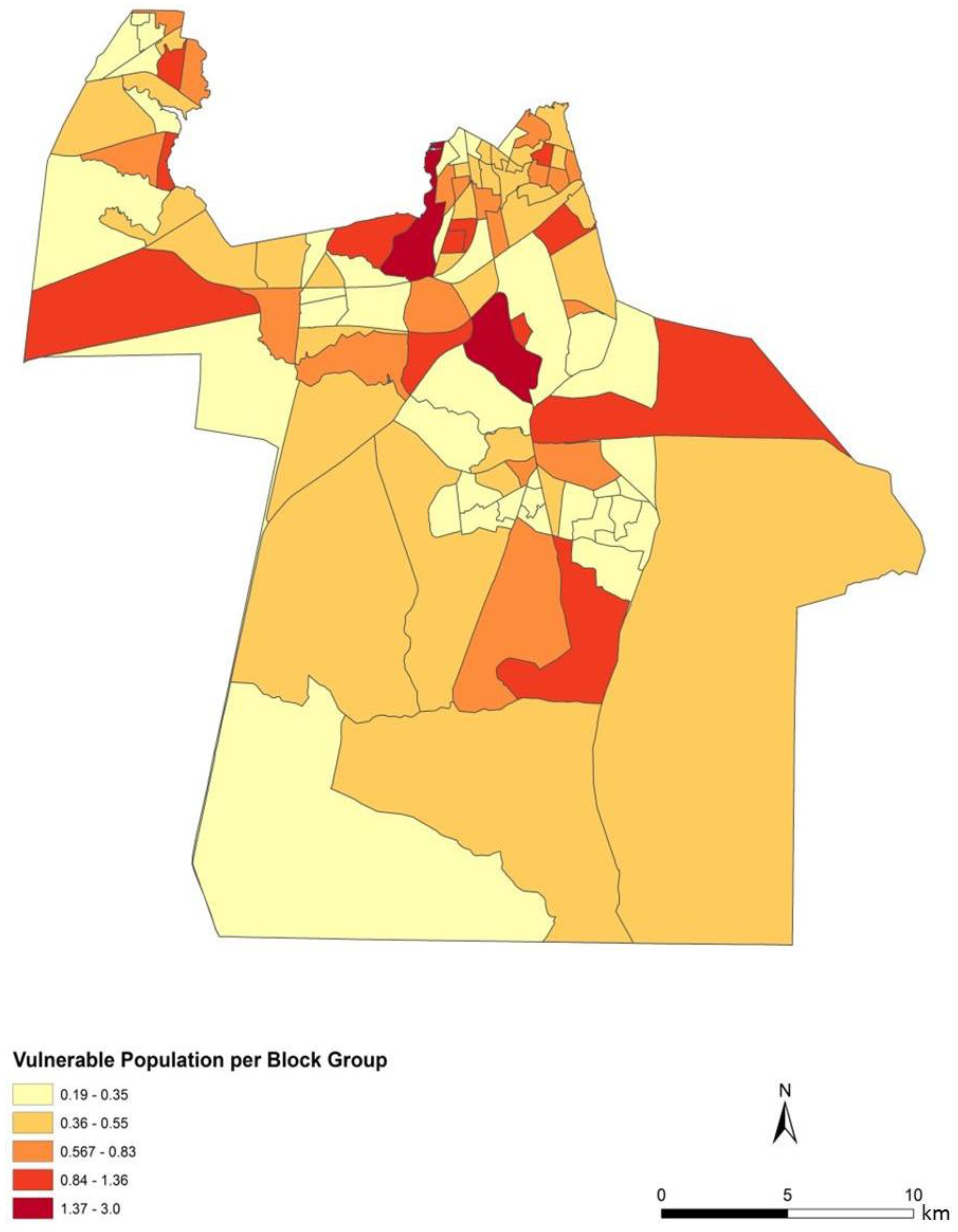
To assess the sensitivity and accuracy of the dasymetric mapping techniques, the raster surface of vulnerability can be compared to the data mapped by block groups. The dasymetric map was expected to provide a more spatially precise representation of population vulnerability as compared to the Census block group choropleths. 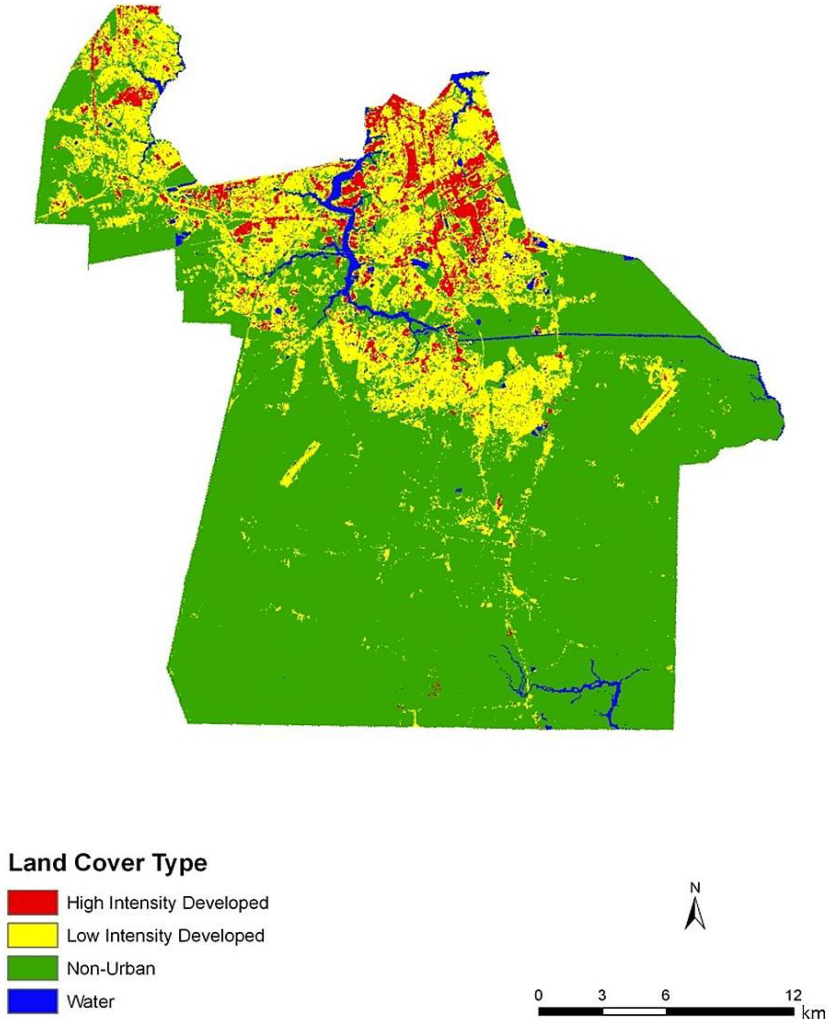Indeed, the block groups show few distinct patterns of vulnerability across Chesapeake (Figure 4). In general, the block groups indicate vulnerability mapped at a coarse scale. 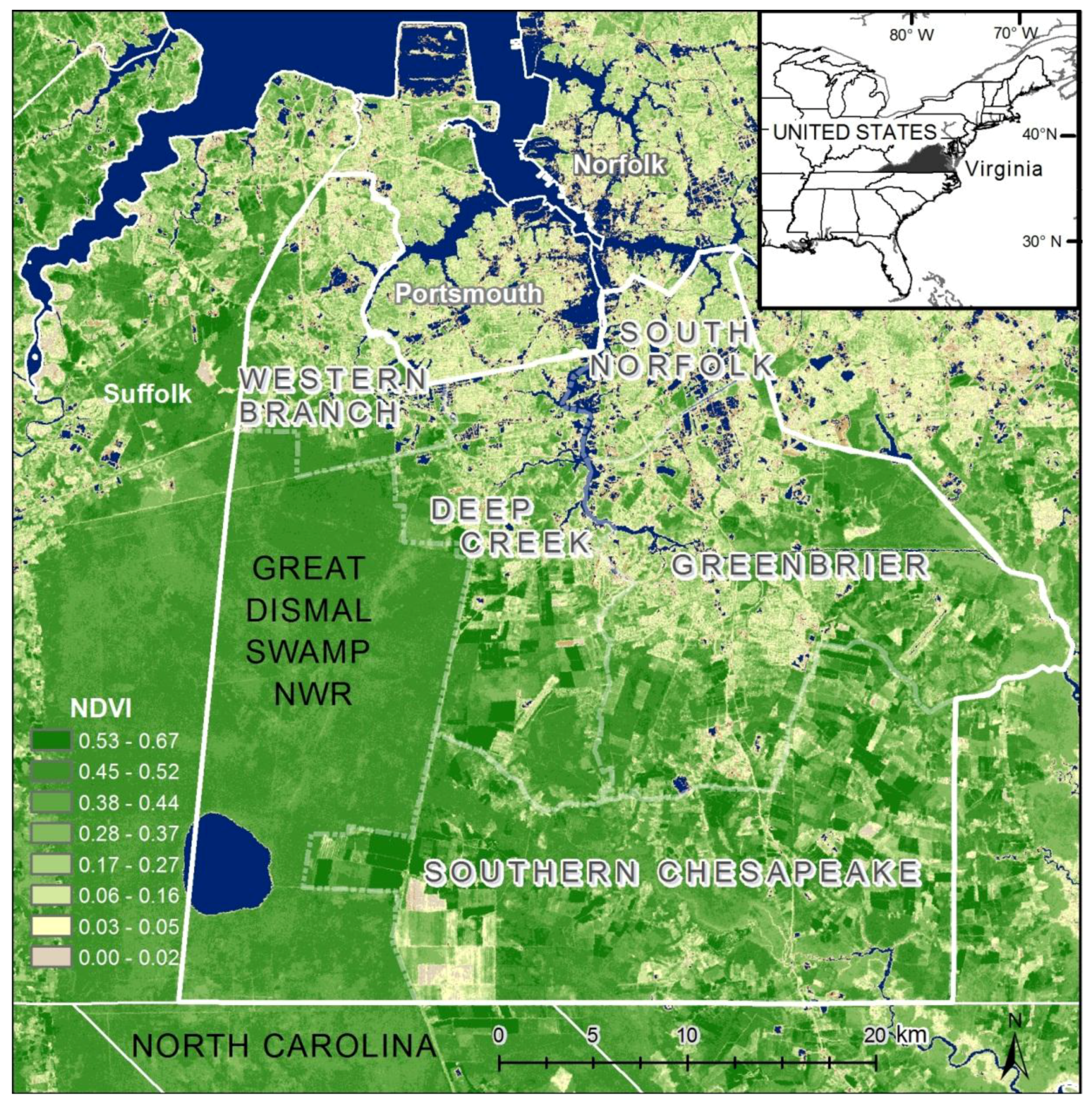Regions of high vulnerability are dispersed and highly concentrated at various locations throughout Chesapeake in block groups, primarily highlighting the urbanized northern and suburban central Chesapeake (Figure 2). 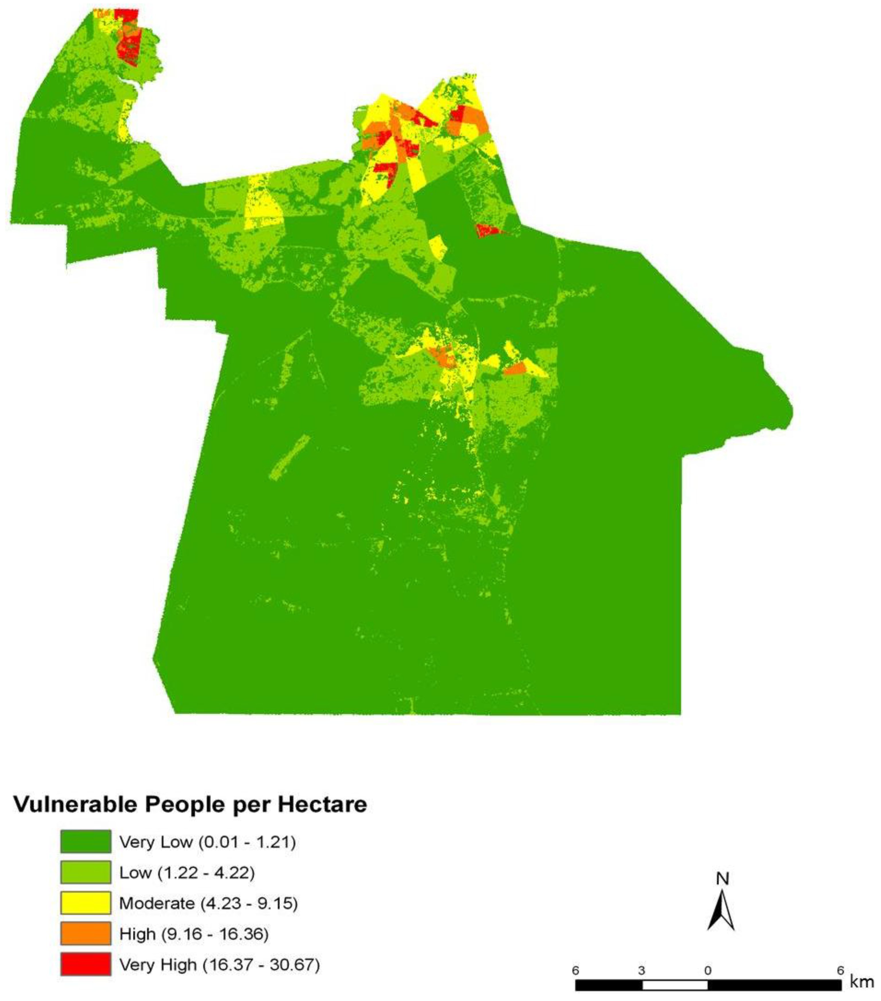Land cover data corroborate this gradient between northern and central, suburban Chesapeake (Figure 3). However, compared to the block group map, the dasymetric map shows a more detailed and fine-scale spatial representation of vulnerability (Figure 7). Again, the highly vulnerable regions are concentrated in the northern portion of the city, but a greater fine-scale pattern and interspersion representing variations are found along arterial transportation routes, major suburban developments, and extensive creek and low floodplain areas. This pattern is mainly attributed to the clustering of vulnerable locations such as schools and daycare centers and surrounding neighborhoods in northern Chesapeake. Northern, urban Chesapeake is more developed than other regions of the city and consequently has a greater population density.

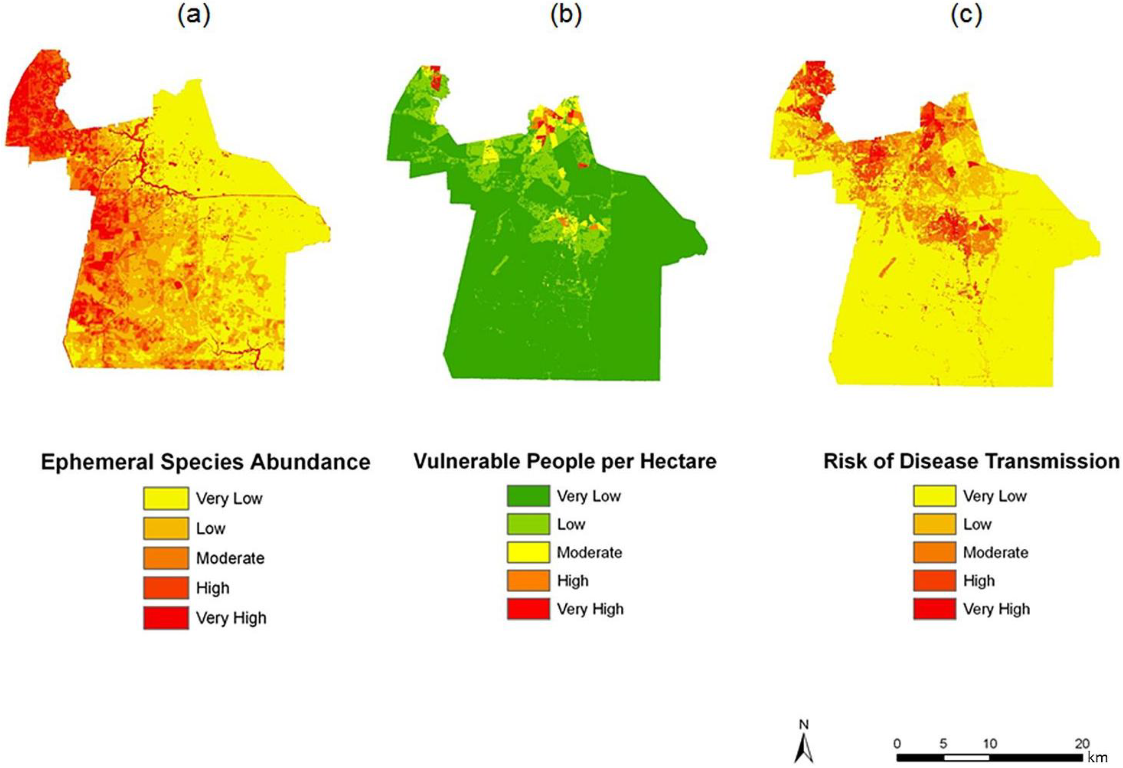
Figure 7. Spatial overlay used to predict potential exposure to ephemeral species for June (a–c). The exposure in June (c) is the product of (a) ephemeral species abundance for that month; and (b) the dasymetric surface of vulnerable population in quantiles.

Figure 7. Spatial overlay used to predict potential exposure to ephemeral species for June (a–c). The exposure in June (c) is the product of (a) ephemeral species abundance for that month; and (b) the dasymetric surface of vulnerable population in quantiles.

Two finer scale patterns of vulnerability are evident across the city. First, regions covered in water or rural areas are populated with a smaller number of vulnerable people. This was expected since these regions are less developed and contain lower disease susceptible populations. Mosquito control personnel interpret the fine-scale patterns of mosquito abundance, vulnerable populations, and composite exposure to assist operational surveillance and abatement activities. In some cases, the proximity of high abundance and high human populations may be amenable to spraying from trucks. In other cases where risk is low to moderate, less frequent spraying or larvicide applications are typically pursued. Second, the high risk indicated in the Western Branch area of Figure 7c has typically spurred routine seasonal spraying, with particular attention to neighborhoods adjoining tidal creeks and the zone between this part of the city and the Great Dismal Swamp. High to very high risk is also noted in the north-central area of Chesapeake, the most urbanized area of the city adjoining the City of Norfolk. Although ephemeral species abundances in the month of June are low, the total population and areal density of human population is extremely high (much higher than the density in the western and southern suburbs.)

Public health and mosquito control specialists treat highly urbanized and dense population centers slightly differently from suburban populations. In this instance, the urbanized areas have permanent surveillance operations in light trapping and inspection of urban ditches, culverts, storm drains, and creeks prevalent in this area. In contrast, suburban surveillance typically comprises fewer and wider spread light traps and the use of periodic roving trapping efforts, as well as a greater dependence on nuisance reports and abatement requests to cover the much greater suburban area. The indices developed here are thus trending toward a persistently higher risk in the more populous urban centers, with more changeable risk in the suburban and rural zones. However, this index could indicate bias that could be construed as a false positive in low mosquito abundance periods or a lack of sensitivity during a rare high abundance bloom event. This concern is somewhat muted in the instance of northern Chesapeake, which also has not only the densest human population, but also a concentration of elderly. Such population densities can have profound effects on potential disease exposure [3].

Other studies have used dasymetric techniques to map population density and have obtained similar results. Many studies have found that dasymetric mapping provides a more accurate representation of population distribution compared to conventional mapping techniques. One study used dasymetric mapping to map population density in five counties within southeast Pennsylvania [16]. Using areal weighting, block group demographic data was mapped according to three classes of urban land cover. The dasymetric map raster was compared to vector population data within block groups. In a similar finding [16], it was observed that within the urban core areas, the choroplethic and dasymetric maps did not differ significantly. However, in areas with parks and cemeteries, the dasymetric map was significantly more detailed. Similar methods were also used to map the San Francisco Bay population by land cover type [13], but rather than using a three-tier classification system, that study used four classes of land cover. Correlation coefficients indicated that the daysmetric mapping method of representing block-group population density was more accurate than the choropleth mapping method. Recent developments have also used address weighting (AW) and parcel distribution (PD) to map rural populations within three North Carolina counties with a focus on using local sources of ancillary data [25]. These mapping techniques are modifications of the existing dasymetric mapping techniques, street weighting (SW) and limiting variable (LV) algorithms. Statistical results indicated that AW and PD were appropriate for mapping rural populations, while SW and LV methods were more effective for mapping the population within urban areas. Yet another approach uses binary dasymetric mapping methods to interpolate populations across regions, such as demonstrated in the county of Leicestershire, England [26]. ArcGIS spatial analyst tools were used to reclassify raster pixel maps as populated or unpopulated. Weighting methods to map Census data have also focused on streets to adjust population across areal units in Los Angeles County, California [27]. Compared to simple aerial interpolation techniques, the dasymetric surface showed a 20% increase in population accuracy. An even finer scale and 3D cadastral-based data have been applied to map the population of New York City [14]. This method disaggregates population data at a high spatial resolution using cadastral data. For this study, residential units (RU) and residential area (RA) were aggregated to the tax lot, block group, and census tract level. The census tract values were then disaggregated to the tax lot level and then re-aggregated to predict the values within each block group. Cadastral-based Expert Dasymetric System (CEDS) derived population values are thus more finely allocated population than census values within block groups. Our results using the dasymetric mapping method corroborate these previously published techniques, highlighting the technique’s potential to illustrate spatial variation and pattern among populations as compared to choroplethic mapping.

4.2. Risk Maps of Mosquito Vector Exposure

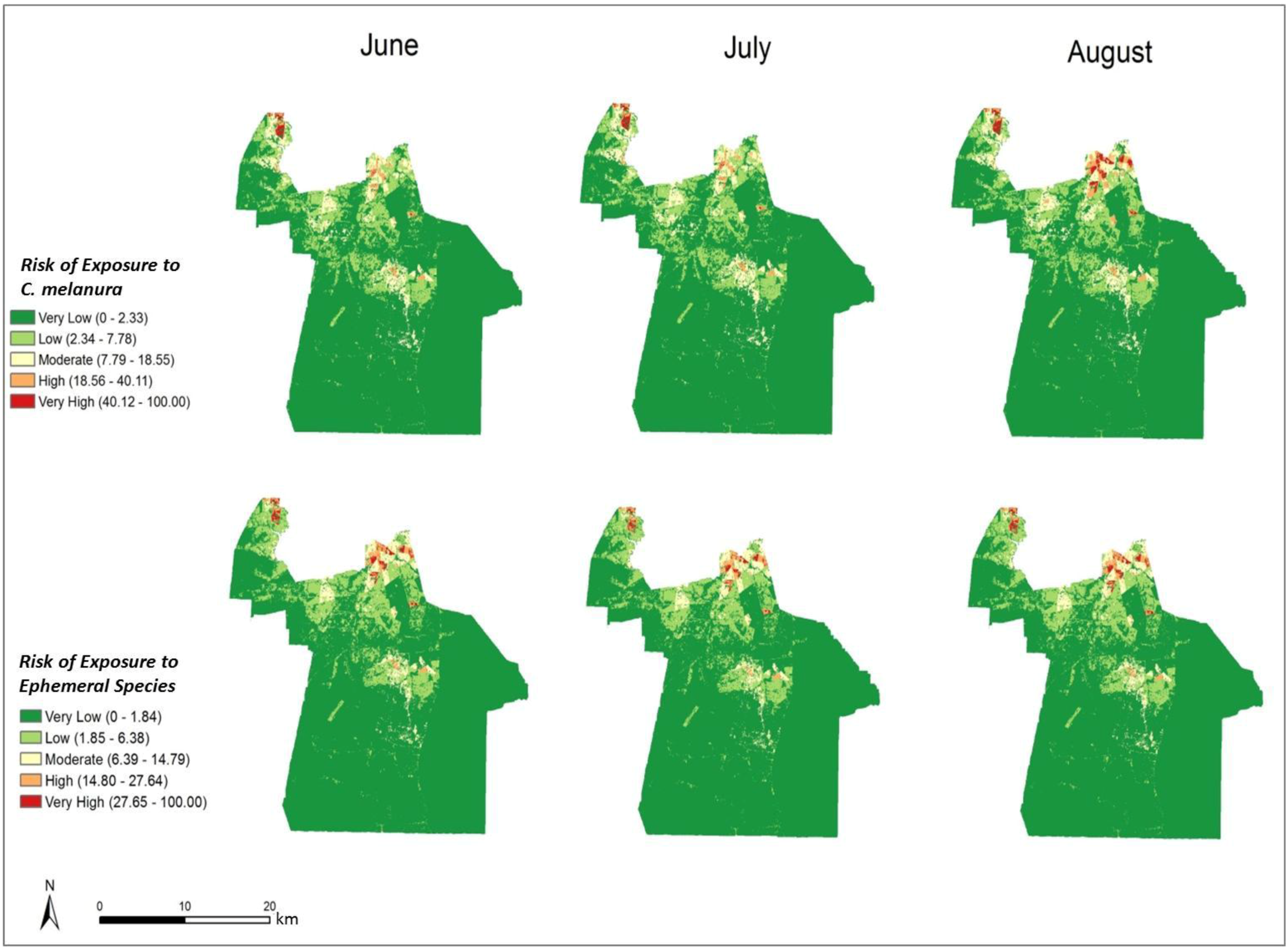
The risk of exposure to mosquito vectors across Chesapeake from both groups of mosquitoes is shown in Figure 8. The risk indices were scaled to show the level of risk for each month. To provide an effective visualization of the risk indices, risk values were classified into quantiles while maintaining each monthly index on the same relative scale. The actual units of risk are arbitrary and represent a relative index ranging from low to high risk. It is apparent on examining the maps that the threat of disease does not change significantly from June through August of 2003. This is due to the relatively static climate (warm and humid) conditions that persisted throughout the summer of 2003. The threat of disease transmission was also very similar between the two species groups. A longer time series or a period with more variable precipitation or weather events inducing mosquito population cycles would have elicited greater temporal variability, as documented in preceding habitat suitability and environmental modeling [4].

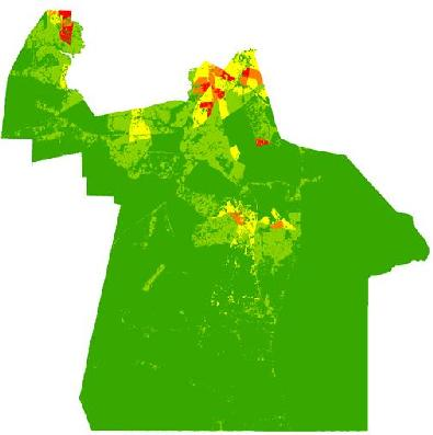
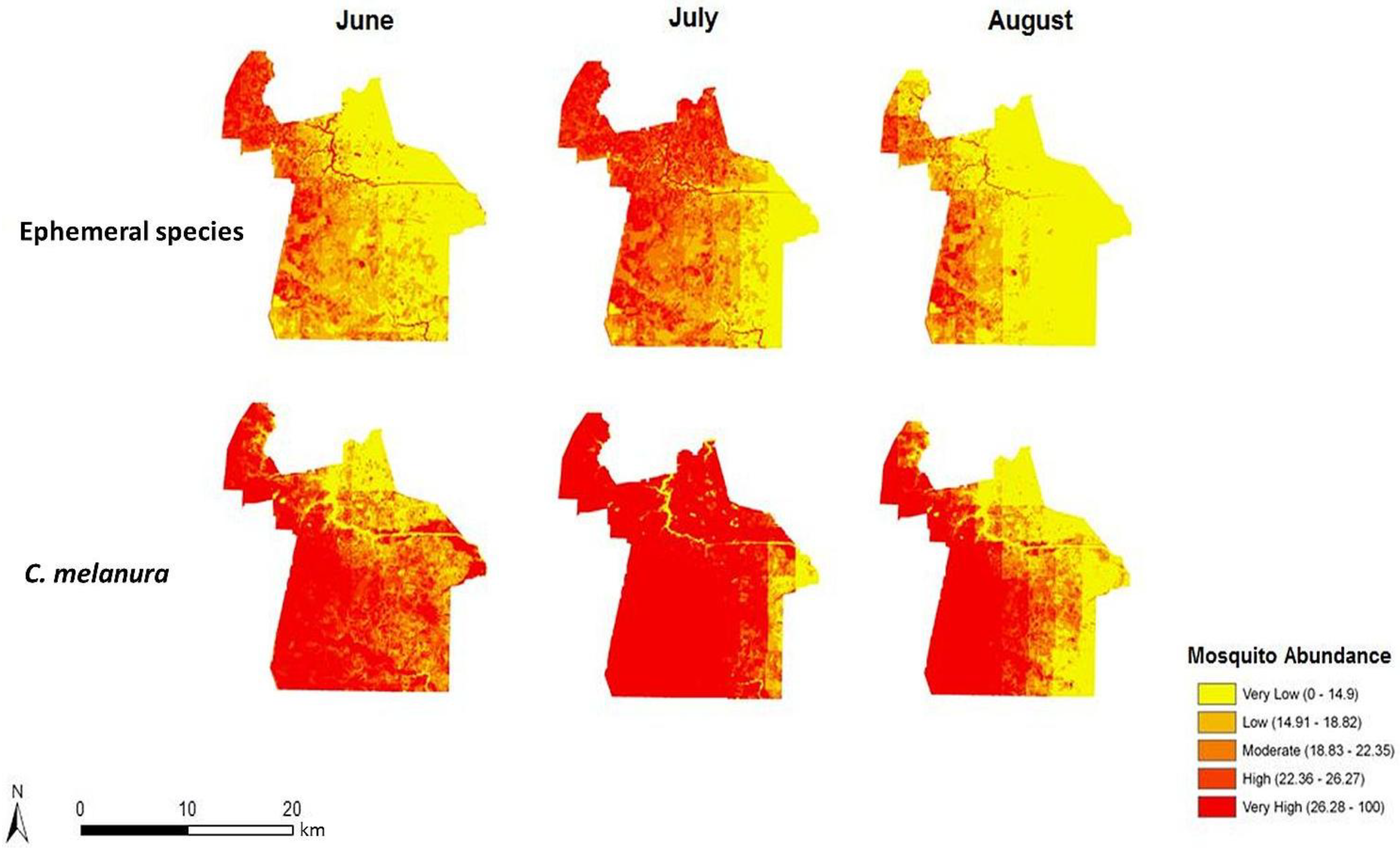
In particular, northern and central Chesapeake have a high risk of exposure to mosquitoes across all summer months. These high risk areas are reflective of the dasymetric map of vulnerability (Figure 5). The high risk regions coincide with regions predicted to have a relatively high vulnerability to disease infection. Despite the elevated risk in these regions, absolute mosquito abundance was predicted to be low in northern Chesapeake (Figure 6). The low number of mosquitoes may be due to the high level of urbanization and less prevalent suitable mosquito habitats or human adaptations to mitigate their abundance (especially reducing container breeding sites.) Although mosquito abundance was estimated to be low in northern Chesapeake, disease transmission levels may nonetheless be relatively high due the greater level of contact with humans in these developed areas. Indeed, cities may generally exacerbate disease transmission by bringing a large number of people into intimate contact with mosquito vectors [28]. Even with a supply of clean water, adequate shelter, and access to health care, a high population density would greatly facilitate the spread of transmissible disease. Despite the low number of swamps and floodplains in these developed regions, mosquitoes may still come into close proximity of humans by other sources of standing water. Ae. Vexans and P. columbiae are typically found in flood plains where rivers overflow their banks, but significant numbers can be produced from virtually any area where water accumulates on an intermittent basis [29]. These mosquitoes may breed in temporary water sources such as drainage ditches and tire ruts, which are extensive in low-lying coastal plains such as Chesapeake.

Figure 8. Monthly indices representing the risk of exposure to mosquito vectors for C. melanura and ephemeral species (values classified using natural breaks and fixed class breaks through time).

Figure 8. Monthly indices representing the risk of exposure to mosquito vectors for C. melanura and ephemeral species (values classified using natural breaks and fixed class breaks through time).

Prior to estimating the vulnerable population, it was expected that regions of high mosquito abundance would coincide with regions of high risk. However, many regions observed to have a high number of mosquitoes such as southern Chesapeake were predicted to have a lower relative risk of exposure. The area surrounding the Great Dismal Swamp, for instance, was observed, as expected, to exhibit high mosquito abundance. Nonetheless, this area exhibits a relatively low disease risk owing to low resident populations. Recreational activities in such swamplands should be considered a significant caveat, as recreational activity spaces (boaters, hikers, bird-watchers, and paddlers) are not characterized in this modeling. Such mosquito-abundant areas are mostly undeveloped and therefore capable of supporting mosquito populations. The climatic variables such as temperature and rainfall were calculated to have a greater effect on the mosquito trap counts in western Chesapeake compared to the rest of the city [4]. These western areas are covered in either wetlands or croplands. The immature stages of mosquitoes require water and therefore are often found in wetlands [30]. The runoff from croplands can also support mosquito presence [31]. Despite these favorable conditions, many of these rural areas have a low human population density and exhibit less total population at risk of disease exposure. Hence, these results highlight that although mosquitoes can transmit disease to humans, without exposure to the pathogen, the likelihood of disease transmission is decreased.

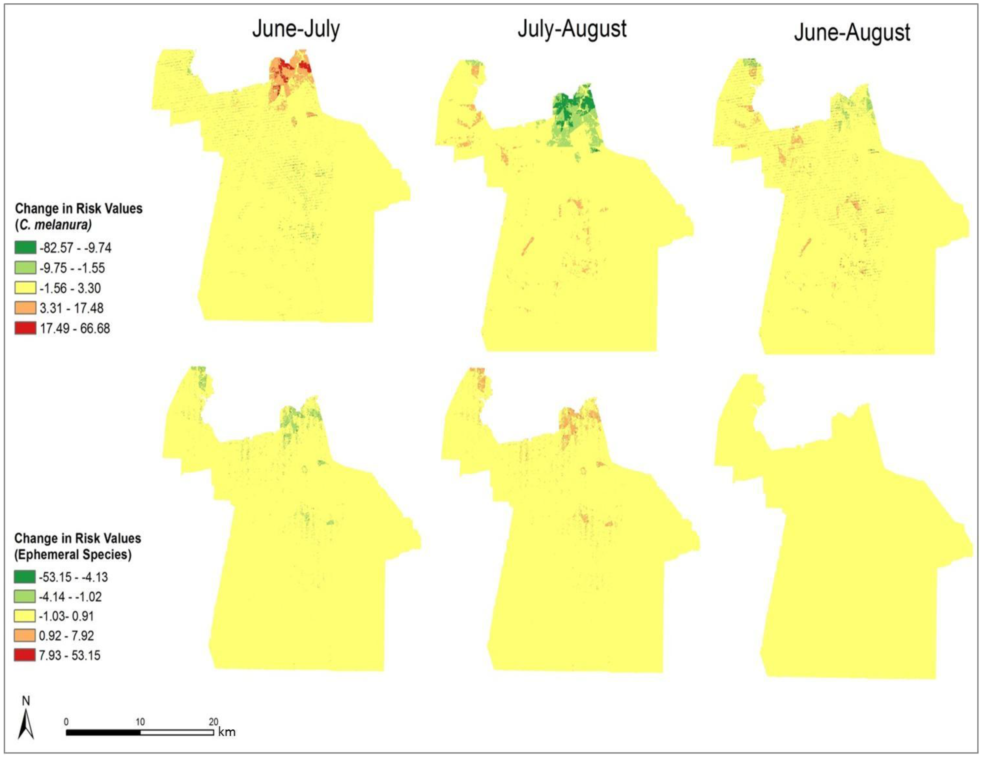
In order to compare the variation in risk from June through August, the differences in the monthly risk indices were calculated. Each month’s risk values were subtracted from the following month’s values to calculate the difference over each month. The results of this calculation are shown in Figure 9 It is clear that the most significant changes in risk occurred in northern Chesapeake. The remaining portion of the city did not show a significant change in risk over the three-month period. From June through July, the risk of exposure from C. melanura increased drastically in northern Chesapeake. Conversely, the risk values for the ephemeral species decreased over this time period. Modest and opposite trends are evident from July through August. For C. melanura, risk decreased in northern Chesapeake, while the risk values for the ephemeral species increased. Overall, there was little variation in risk between June and August. C. melanura showed minimal change, while the ephemeral species showed almost no change in risk values.

Validation of trends in abundance and population exposure is a challenging proposition in the instance of rare disease and a complex mosaic landscape such as Chesapeake. No human cases of West Nile Virus or EEE were reported in Chesapeake during the season studied. However, The Virginia Department of Public Health later reported (2004) [32] that 20 pools of mosquitoes were found to be positive for C. melanura infected with EEE, while 10 pools were positive for West Nile. Additional surveillance and nuisance abatement request data were provided by the City of Chesapeake and offer limited affirmation of the risk mapped. While not validated, some studies have found that animal cases can be accurate indicators of human disease prevalence [33]. 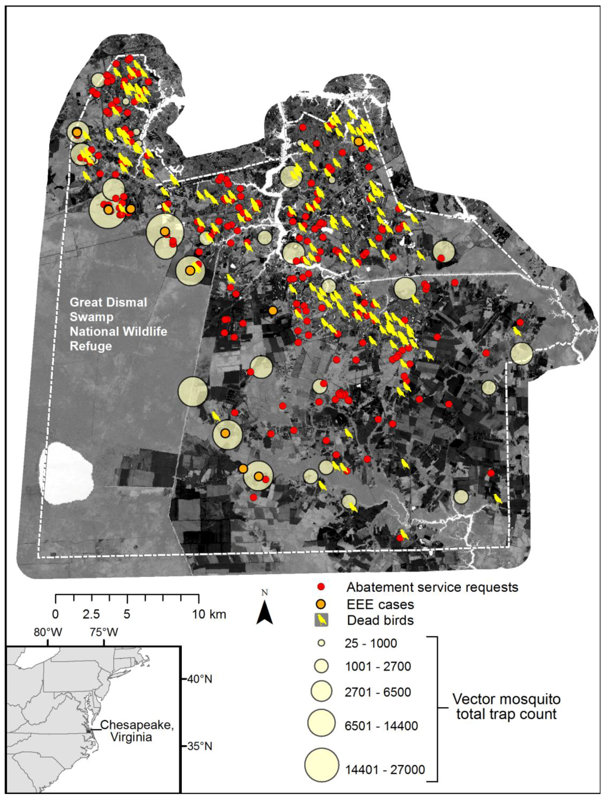Figure 10 depicts a composite of available information, including total vector species trap counts over the season, dead bird reports (a majority of crows), and cases of Eastern Equine Encephalitis (EEE) among horse farms. Although an exhaustive map of horse farms was not available, EEE incidents are coincident with the highest vector abundance data. Further, the abatement service requests and pattern of dead birds collected (initially many of these were tested for WNV), also spatially conforms to the dasymetric population map and human exposure risk. Figure 9 also illustrates the dilemma of solely relying upon discovery of surveillance tools such as dead birds or resident reported abatement requests, as these patterns reflect the abundance of humans and not necessarily the abundance of mosquito vector species.

It is difficult to validate such risk models due to the low number of disease cases and underreporting. Disease surveillance data do not record any actual human cases of WNV or EEE occurring in Chesapeake in 2003. However, in 2003, 20 pools of mosquitoes were found to test positive for C. melanura infected with EEE, while 10 pools were infected with C. melanura positive for WNV [32]. These corroborating data, combined with the usual under-reported and underdiagnosed nature of WNV, suggest that C. melanura mosquitoes were an emerging health threat to Chesapeake in 2003. In addition, bird, equine, and sentinel flock cases of WNV and EEE were reported for this year. These cases may not provide a validation of the model since the model estimates risk to humans, rather than animal hosts, but they do lend some credence and affirmation to the risk mapping approach. A plausible spatial relationship can be seen between EEE cases and C. melanura abundance. In 2003, the majority of EEE cases occurred in western Chesapeake, surrounding the Dismal Swamp, and our abundance mapping of the EEE vector C. melanura was also predicted to be high in western Chesapeake from June through August. The high predicted abundance of mosquito vectors, observations in traps, and resident abatement requests also lend credence to inference of higher risk exposure.

Figure 9. Change in monthly exposure risk values through the summer derived by calculating the difference in the risk indices shown in Figure 8.

Figure 9. Change in monthly exposure risk values through the summer derived by calculating the difference in the risk indices shown in Figure 8.

Dasymetric mapping is shown in this investigation to be effective at representing population data as compared to mapping by areal choropleths such as Census block groups for population vulnerability and exposure assessment. The choroplethic map of vulnerability in Census units (Figure 9) gives the impression that the population is homogenously distributed within each block group, yet proportions of each block group are extensively uninhabited. The dasymetric map on the other hand (Figure 8), shows vulnerability at a finer scale and with many localized patterns and concentrations among urban, suburban, and rural settlements. By using pixels as the areal units rather than block groups, the raster shows a continuous and variable surface of vulnerability. By integrating the “nighttime” population values from the Census data with the point-based nodes of vulnerability to produce the vulnerability index, the resulting population risk map is likely to have a higher accuracy than results generated from considering the Census data alone.

Figure 10. Seasonal mosquito vector trap counts, enzootic disease reports (dead birds and veterinary surveillance of positive EEE horses), and public abatement service requests within Chesapeake, over Landsat TM tasseled cap wetness index image for 29 July 2002.

Figure 10. Seasonal mosquito vector trap counts, enzootic disease reports (dead birds and veterinary surveillance of positive EEE horses), and public abatement service requests within Chesapeake, over Landsat TM tasseled cap wetness index image for 29 July 2002.

This study affirms the role of demographic data and spatial analysis for mapping and predicting the risk of mosquito vector exposure. Due to the many factors affecting disease transmission, vector abundance and exposure may not be positively correlated with general areal risk of exposure. Although exposure to mosquitoes may be high in some regions across Chesapeake, disease transmission may not necessarily be high due to the low population density in these regions. This study supports the importance of incorporating human data in addition to climate data when predicting risk and may be used as a guide to strategically allocate surveillance and control activities over space. Ancillary enzootic data from dead birds and EEE cases as well as nuisance abatement requests support the inference of geographic gradients of vector abundance and possible exposure risk. Future studies may consider incorporating other human factors such as behavior, disease resistance, and socioeconomic data. According to Daily and Ehrlich [28], “human demographic factors are key variables in epidemiology, influencing the rate at which a population is invaded by new parasites, their chances of becoming established, the rate of their spread, the evolution of their virulence, and the capacity of human social structures (and other cultural traits) to coevolve in defense”. The lack of fine-scale human population data was considered a limiting factor in the initial development of dasymetric maps, yet future studies should more carefully assess the role of scale in both vector abundance as well as susceptible populations.

Further considerations of disease transmission factors could improve similar research. For instance, it is possible that scale issues of human settlements and activity species and the vectors could be individually better understood and that fine-scale data (of either factor) may not add additional value to surveillance or control. Other factors, which influence vector exposure and disease transmission, may also be incorporated into future studies. Deforestation, for instance, can lead to environmental changes conducive to mosquito survival [30]. Vector competence, for example, could also be used to help predict the rate of transmission, and studies have begun to explore the relationship between West Nile virus, climate change [34], and specific vector competence of Culiseta incidens and Culex thriambus [35] and the variation in vector competence of Culex pipens across California [36]. Further, climate change, particularly extreme heat, rainfall, and rising sea levels, is poised to alter the habitats, suitability, and potential human settlement patterns in low-lying areas such as Chesapeake.

The geospatial methods used in this study may be beneficial to other cities afflicted by vector-borne diseases and extreme weather events. In rich and poor nations alike, cities are afflicted by a lack of control over disease reservoirs and vectors [28]. Predicting where mosquito-borne diseases pose the greatest risk to human health could improve spatial precision of mosquito control efforts and thereby reduce costs and impacts of broader insecticide use. GIS has been demonstrated as highly useful in emergency operational assessment of control methods, such as estimating areal needs for aerial or ground-based spraying, including distance and drive-times [37].

5. Conclusions

As vector-borne diseases continue to persist, many researchers and healthcare officials are concerned with estimating and mapping disease risk. Many spatial risk assessments rely solely on vector presence to predict disease risk. Using only vector presence to estimate risk can be constraining because mosquitoes are influenced by many interacting factors, particularly climatic variables [33]. By incorporating human vulnerability into a spatial model of disease risk, geographic variations in potential disease transmission can provide health surveillance and mosquito control officials greater information compared to monitoring vectors and environmental factors alone. By identifying high-risk areas in advance, health officials may also reduce disease transmission rates. Emergency managers can target where to implement early-warning systems and risk management procedures in high mosquito abundance habitats in proximity to vulnerable populations following hurricane landfall and flooding (e.g., aerial spraying, larviciding, and emergency shelter site selection). Knowing human exposure and where infectious diseases are likely to emerge could also aid health practitioners in diagnosing and treating patients promptly. With improved data and spatial analytic tools public health managers may apply such spatial risk maps and models to their jurisdictions to reduce the chances of disease.

References

1. Kitron, U. Risk maps: Transmission and burden of vector-borne diseases. Parasitol. Today 2000, 16, 324–325. [Google Scholar] [CrossRef]
2. Mather, F.J.; White, L.E.; Langlois, E.C.; Shorter, C.F.; Swalm, C.M.; Shaffer, J.G.; Hartley, W.R. Statistical methods for linking health, exposure, and hazards. Environ. Health Perspect. 2004, 112, 1440–1445. [Google Scholar] [CrossRef]
3. Sutherest, R.W. Global change and human vulnerability to vector-borne diseases. Clin. Microbiol. Rev. 2004, 17, 136–173. [Google Scholar] [CrossRef]
4. Cleckner, H.L.; Allen, T.A.; Bellows, A.S. Remote sensing and modeling of mosquito bundance and habitats in coastal Virginia, USA. Remote Sens. 2011, 3, 2663–2681. [Google Scholar] [CrossRef]
5. Bellows, A.S. Modeling Habitat and Environmental Factors Affecting Mosquito Abundance in Chesapeake, Virginia. Ph.D. Dissertation, Old Dominion University, Norfolk, VA, USA, 2007. [Google Scholar]
6. Ozdenerol, E.; Taff, G.N.; Akkus, C. Exploring the spatio-temporal dynamics of reservoir hosts, vectors, and human hosts of West Nile Virus: A review of the recent literature. Int. J. Environ. Res. Public Health 2013, 10, 5399–5432. [Google Scholar] [CrossRef]
7. Liu, H.; Weng, Q.; Gaines, D. Spatio-temporal analysis of the relationship between WNV dissemination and environmental variables in Indianapolis, USA. Int. J. Health Geogr. 2008, 7, 66. [Google Scholar] [CrossRef]
8. McKnight, K.P.; Messina, J.P.; Shortridge, A.M.; Burns, M.D.; Pigozzi, B.W. Using volunteered geographic information to assess the spatial distribution of West Nile Virus in Detroit, Michigan. Int. J. Appl. Geospatial Res. 2011, 2, 72–85. [Google Scholar] [CrossRef]
9. Behrens, J.J.; Moore, C.G. Using geographic information systems to analyze the distribution and abundance of Aedes aegypti in Africa: The potential role of human travel in determining the intensity of mosquito infestation. Int. J. Appl. Geospatial Res. 2013, 4, 9–38. [Google Scholar] [CrossRef]
10. Ceccato, P.; Connor, S.J.; Jeanne, I.; Thomson, M.C. Application of geographical information systems and remote sensing technologies for assessing and monitoring malaria risk. Parassitologia 2005, 47, 81–96. [Google Scholar]
11. Beck, L.R.; Rodriguez, M.H.; Dister, S.W.; Rodriguez, A.D.; Washino, R.K.; Roberts, D.R.; Spanner, M.A. Assessment of a remote sensing-based model for predicting malaria transmission risk in villages of Chiapas, Mexico. Am. J. Trop. Med. Hyg. 1994, 56, 96–106. [Google Scholar]
12. Wilson, M.L. Emerging and vector-borne diseases: Role of high spatial resolution and hyperspectral images in analyses and forecasts. J. Geogr. Syst. 2002, 4, 31–42. [Google Scholar] [CrossRef]
13. Sleeter, R. Dasymetric Mapping Techniques for the San Francisco Bay region, California. In Proceedings of the Annual Conference on Urban and Regional Information Systems Association; Reno, NV, USA, 7–10 November 2004. Available online: http://geography.wr.usgs.gov/science/dasymetric/data/URISA_Journal.pdf (accessed on 13 November 2013).
14. Maantay, J.A.; Maroko, A.R.; Herrmann, C. Mapping population distribution in the urban environment: The cadastral-based expert dasymetric system (CEDS). Cartogr. Geogr. Inf. Sci. 2007, 34, 77–102. [Google Scholar]
15. Eicher, C.L.; Brewer, C.A. Dasymetric mapping and areal interpolation: Implementation and evaluation. Cartogr. Geogr. Inf. Sci. 2001, 28, 125–138. [Google Scholar] [CrossRef]
16. Mennis, J. Generating surface models of population using dasymetric mapping. Prof. Geogr. 2003, 55, 31–42. [Google Scholar]
17. Mennis, J.; Hultgren, T. Intelligent dasymetric mapping and its application to areal interpolation. Cartogr. Geogr. Inf. Sci. 2006, 33, 179–194. [Google Scholar] [CrossRef]
18. Gregory, I.N. An Evaluation of the Accuracy of the Areal Interpolation of Data for the Analysis of Long-Term Change in England and Wales. In Proceedings of the 5th International Conference on GeoComputation, University of Greenwich, London, UK, 23–25 August 2000.
19. Smith, C.M.; Graffeo, C.S. Regional impact of Hurricane Isabel on emergency departments in coastal southeastern Virginia. Vet. Res. Commun. 2005, 12, 1201–1205. [Google Scholar]
20. Chesapeake Mosquito Control Commission. 2010. Available online: http://www.chesapeake.va.us/services/depart/mosquito/index.shtml (accessed on 27 March 2012).
21. Zielinksi-Gutierrez, E. West Nile Virus & Other Mosquito-Borne Infections. In The Health Care of Homeless Persons, Part 1, Mosquito-Borne Infections; O’Connell, J.J., Ed.; Boston Health Care for Homeless Program: Boston, MA, USA, 2004; pp. 181–186. [Google Scholar]
22. Shea, K.M. Global climate change and children’s health. Pediatrics 2007, 120, e1359–e1367. [Google Scholar] [CrossRef]
23. Lindsey, N.P.; Staples, J.E.; Lehman, J.A.; Fischer, M. Surveillance for human West Nile virus disease—United States, 1999–2008. Morb. Mortal. Wkly. Rep. 2010, 59, 1–17. [Google Scholar]
24. US Geological Survey. Dasymetric Mapping Tool—ArcGIS 10. 2012. Available online: http://geography.wr.usgs.gov/science/dasymetric/data.htm (accessed on 29 March 2013). [Google Scholar]
25. Tapp, A.F. Areal interpolation and dasymetric mapping methods using local ancillary data sources. Cartogr. Geogr. Inf. Sci. 2010, 37, 215–228. [Google Scholar] [CrossRef]
26. Langford, M. Rapid facilitation of dasymetric-based population interpolation by means of raster pixel maps. Comput. Environ. Urban Syst. 2007, 31, 19–32. [Google Scholar] [CrossRef]
27. Reibel, M.; Bufalino, M.E. Street weighted interpolation techniques for demographic count estimation in incompatible zone systems. Environ. Plan. 2005, 37, 127–131. [Google Scholar] [CrossRef]
28. Daily, G.C.; Ehrlich, P.R. Global change and human susceptibility to disease. Annu. Rev. Energy Environ. 1996, 21, 125–144. [Google Scholar] [CrossRef]
29. Crans, W.G. A classification system for mosquito life cycle: Life cycle types for mosquitoes of the northeastern United States. J. Vector Ecol. 2004, 29, 1–10. [Google Scholar]
30. Dale, P.E.R.; Knight, J.M. Wetlands and mosquitoes: A review. Wetl. Ecol. Manag. 2008, 16, 255–276. [Google Scholar] [CrossRef]
31. Ward, M.P.; Wittich, C.A.; Fosgate, G.; Srinivasan, R. Environmental risk factors for equine West Nile Virus disease cases in Texas. Vet. Res. Commun. 2009, 33, 461–471. [Google Scholar] [CrossRef]
32. Virginia Department of Health. Arbovirus Data 2003. Available online: http://www.vdh.virginia.gov/epidemiology/DEE/Vectorborne/arboviral/documents/testresults/2003.html (accessed on 12 March 2004).
33. Eidson, M.; Komar, N.; Sorhage, F.; Nelson, R.; Talbot, T.; Mostashari, F.; Mclean, R. West Nile Virus Avian Surveillance Group. Crow deaths as a sentinel surveillance system for West Nile Virus in the northeastern United States. Emerg. Infect. Dis. 1999, 7, 615–620. [Google Scholar]
34. Gage, K.L.; Burkot, T.R.; Eisen, R.R.; Hayes, E.B. Climate and vectorborne diseases. Am. J. Prev. Med. 2008, 35, 436–450. [Google Scholar] [CrossRef]
35. Reisen, W.K.; Fang, Y.; Martinez, V.M. Vector competence of Culiseta incidens and Culex thriambus for West Nile virus. J. Am. Mosq. Control Assoc. 2006, 22, 662–665. [Google Scholar] [CrossRef]
36. Vaidyanathan, R.; Scott, T.W. Geographic variation in vector competence for West Nile Virus in the Culex pipiens (Diptera: Culicidae) Complex in California. Vector Borne Zoonotic Dis. 2007, 7, 193–198. [Google Scholar]
37. Mak, S.; Buller, M.; Furnell, A.; MacDougall, L.; Henry, B. Use of geographic information systems to assess the feasibility ground- and aerial-based adulticiding for West Nile Virus control in British Columbia, Canada. J. Am. Mosq. Control Assoc. 2007, 23, 396–404. [Google Scholar] [CrossRef]