
Transport Accessibility Analysis Using GIS: Assessing Sustainable Transport in London


Abstract
:
1. Introduction
2. Measuring Transport Costs and Accessibility
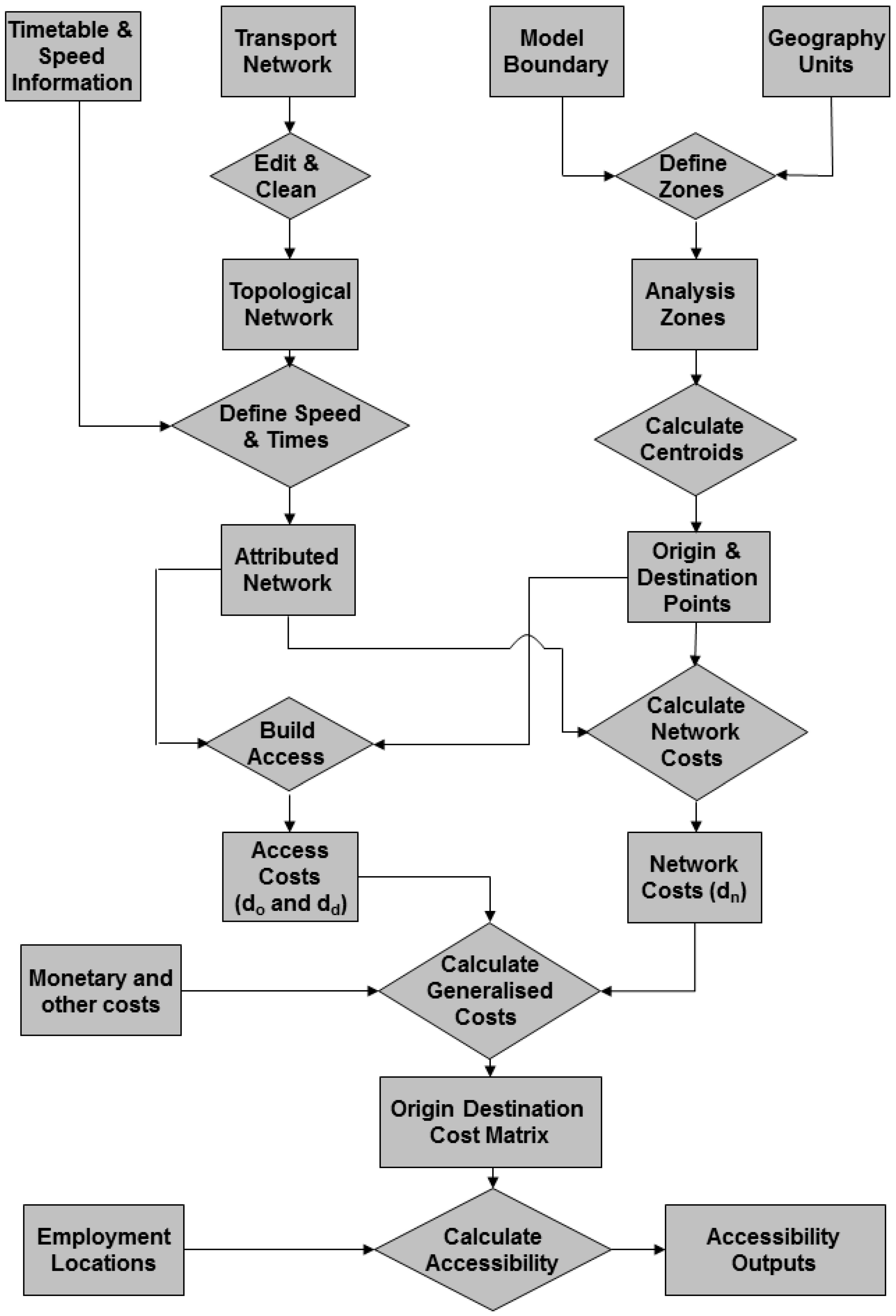
3. Implementation of GIS-Based Model

- First, the spatial geography of the model is defined in terms of zonal geography and the spatial boundary of analysis (for example for the London case study presented below, these are UK Census Area Statistics Wards, i.e., zones on which 2001 UK census outputs are reported).
- Build M transport networks:
- Analyze, and clean if necessary, the data to ensure the correct topological structure for creation of a spatial network model.
- Build spatial networks within GIS software.
- Calculate the length of each network link from geometry.
- Multiply each network link length by the relevant travel speed to obtain the travel time for each link.
- For N units of spatial geography, create an N x N matrix of generalized costs for each of the M transport modes (similar to the approach outlined by Benenson et al. [24]):
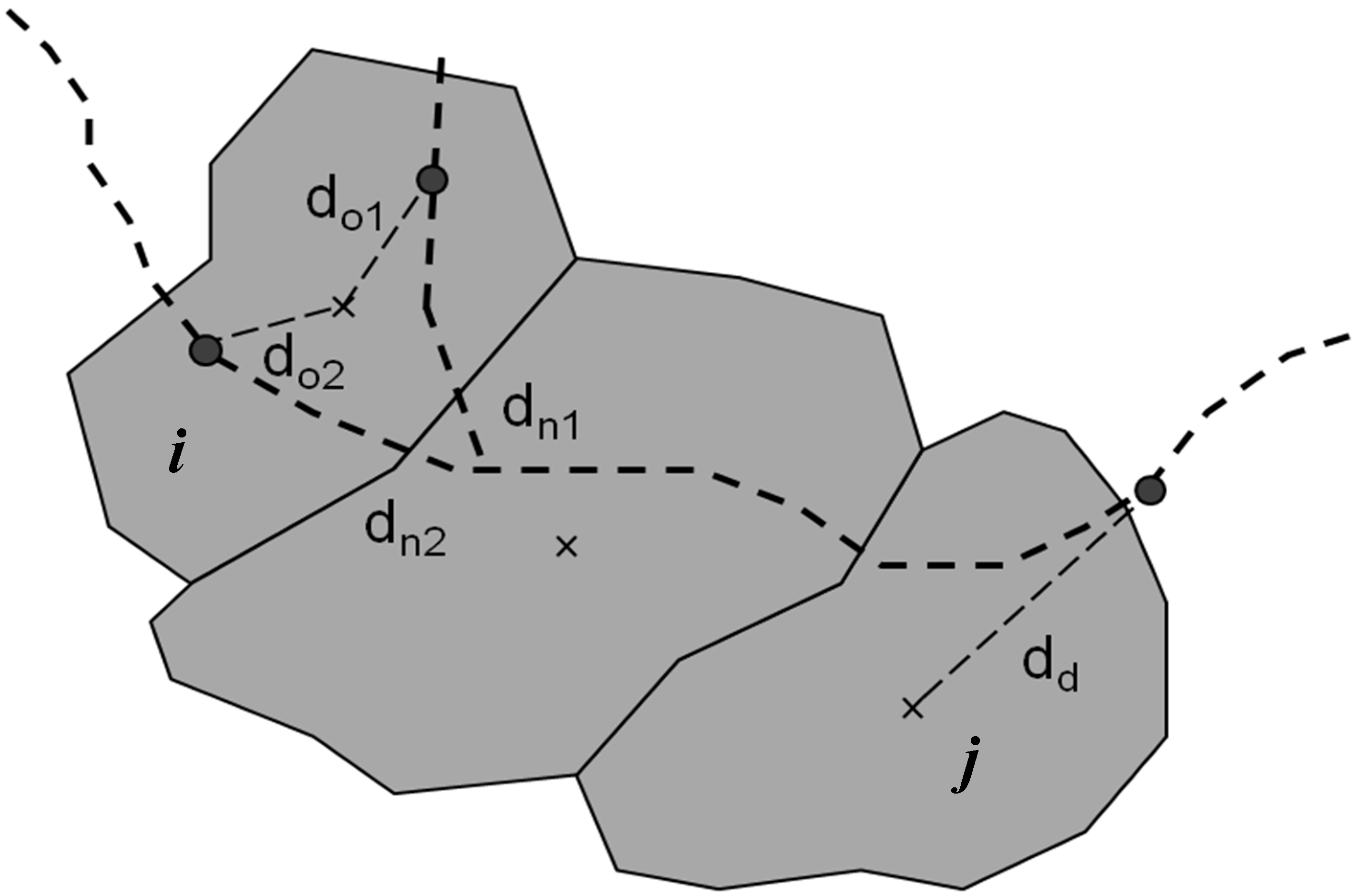
- Calculate the location of the centroid and use it to define the Origin, and Destination of zone i.
- Calculate access distance, do, and associated travel time from centroid to nearest network access location (private and cycling modes), or boarding point (public transport modes) (Figure 2)
- Calculate access distance, dd, and associated travel time from destination station or stop (public transport) or road access location (private and cycling modes) (alighting point) to the centroid of the destination zone (Figure 2).
- Eliminate nonsensical journeys (e.g., where nearest station is shared between the origin and destination) and return a no-data value.
- Add on other costs, including non-monetary and monetary components in Equations (4a)–(4c) such as fuel or perception weights, converted to time.
- Sum all journey components to calculate the generalized cost of travel, Cij, between two zones.
- For situations where i = j and the preceding steps calculate Cij = 0 then assume that in line with the approach used by Feldman et al. [49].
- Use computed generalized costs to determine accessibility to destinations of interest (e.g., employment locations) and determine the proportion of employment which is accessible by a given mode in a given cost of travel.


| T2025 Scenario | Road | Bus | Rail | Light Rail |
|---|---|---|---|---|
| Baseline | Crossrail High Speed 1 Heathrow Express to Terminal 5 | Heathrow Terminal 5 extension | ||
| Low | Thames Gateway Bridge | 20% increase in bus supply (and thus frequency) | Reduce journey time by 4.5% | DLR extensions, Greenwich and East London transit systems |
| High | Silvertown Link Bridge National Road User-charging scheme | 40% increase in bus supply. | Crossrail 2, East London line extension (Overground). | Tramlink extensions, DLR extension to Dagenham Dock |
| Parameter | Description | Value Used in Analysis |
|---|---|---|
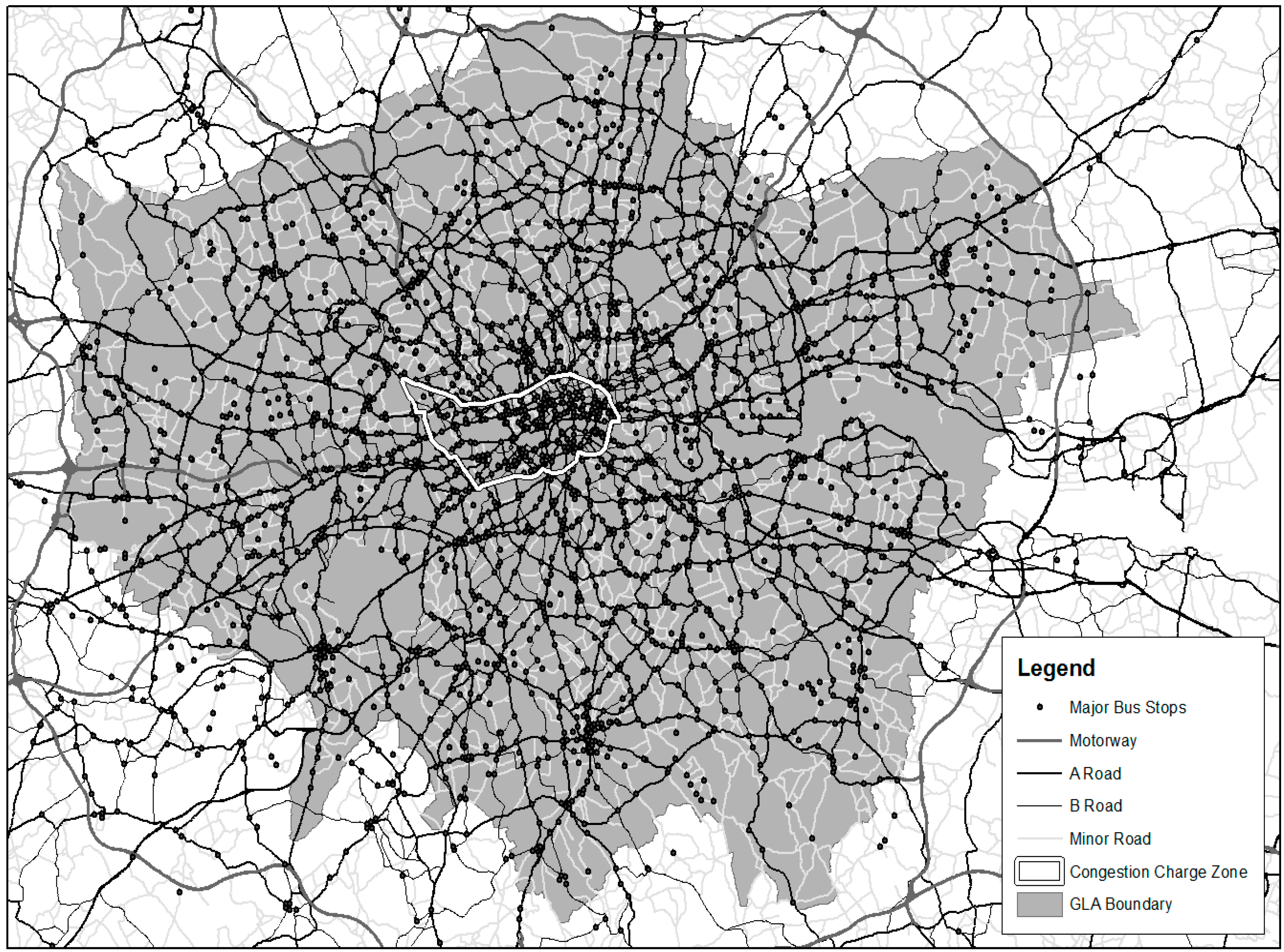
| A | Time take to access a given transport network mode from a place of residence. This uses do and dd which are the distance from the transport mode to the zone centroid (Figure 2). | Private transport modes: 3 min - the maximum access distance in Greater London is 800 m (in the Hillingdon ward in western Outer London), with the mean distance being 130 m.
Public transport modes: Distance from zone centroid to station, with a walking speed of 6 km/h |
| Vwk | Weight applied to the walking component of a journey to reflect the increased perceived cost of walking compared to other transport modes (applied to do and dd). | 1.6 from WEBTAG [41] |
| T | The in-vehicle travel time is computed by multiplying the network distance by an average speed. This is the time taken to travel distance dn. | Computed from network analysis described in Section 2.
Car: defined by 2006 London Travel Report Table 3.2.1, which gives the average journey speed for three traffic zones; central, inner and outer London [52]. Heavy rail: 40 km/h Light rail: 30 km/h Bus: times supplied in network data |
| W | Waiting time is calculated as half the average morning peak service frequency for public transport modes. | Rail: 7.5 min
Light rail: 3 min Bus: 3 min |
| Vwt | Weight applied to any waiting time, reflecting the perceived cost of waiting compared to travelling, and a dislike of waiting for infrequent services. | 2.6 from WEBTAG [41] |
| D | Distance travelled (km) traversing the least cost path from origin to destination, and is equivalent to dn (Figure 2). | Computed from network analysis. |
| VOC | Vehicle Operating Cost is the sum of both fuel, VOCf, and non-fuel, VOCnf, costs (which capture maintenance and depreciation costs). | Fuel costs, where Fm is a vector of the vehicle mix and their fuel efficiency and Fp is a vector of fuel prices. Non-fuel operating costs can be computed by the following: where V = average velocity in km/h; a1 = 4.069; b1 = 111.391. |
| VOT | Value of Time. | 1 hour = £5.04 from WEBTAG [41] |
| occ | Average number of occupants in a private vehicle. | 1.16 people per vehicle [41] |
| PC | Other private transport costs. Information on parking costs and policies was incomplete for London so have not been included in this analysis. However, the London Congestion Charge, levied on vehicles entering the center of the city, has been included. | Congestion Charge of £8 (2008 charge) levied on each journey into the charging zone. 90% discount for residents of the zone travelling out for work [53]. |
| F | The fare paid for a given origin-destination route varies according to the time of day and whether the individual has a season ticket, travel card, or uses an “Oyster Card”. An average rail and light rail cost is reported in the London Travel Report (TfL, 2006). Flat bus fares £2, or £1 with an “Oyster Card”. However, 85% of journeys (TfL, 2007) use an Oyster Card so this was used for all journeys in this analysis. | Heavy and light rail: £0.18/km
Bus: £1 flat fare |
| VTopo | It is assumed that cycling journeys incur a lower cost on flatter terrain than on more undulating terrain. In this paper, a modified version of Naismith’s Rule is used, where each unit of vertical change adds 1/8th of a unit of horizontal distance to the journey. | 1/8 * (Zmax − Zmin) for a given road link, where Zmax and Zmin are the maximum and minimum elevations at either end of the link. |
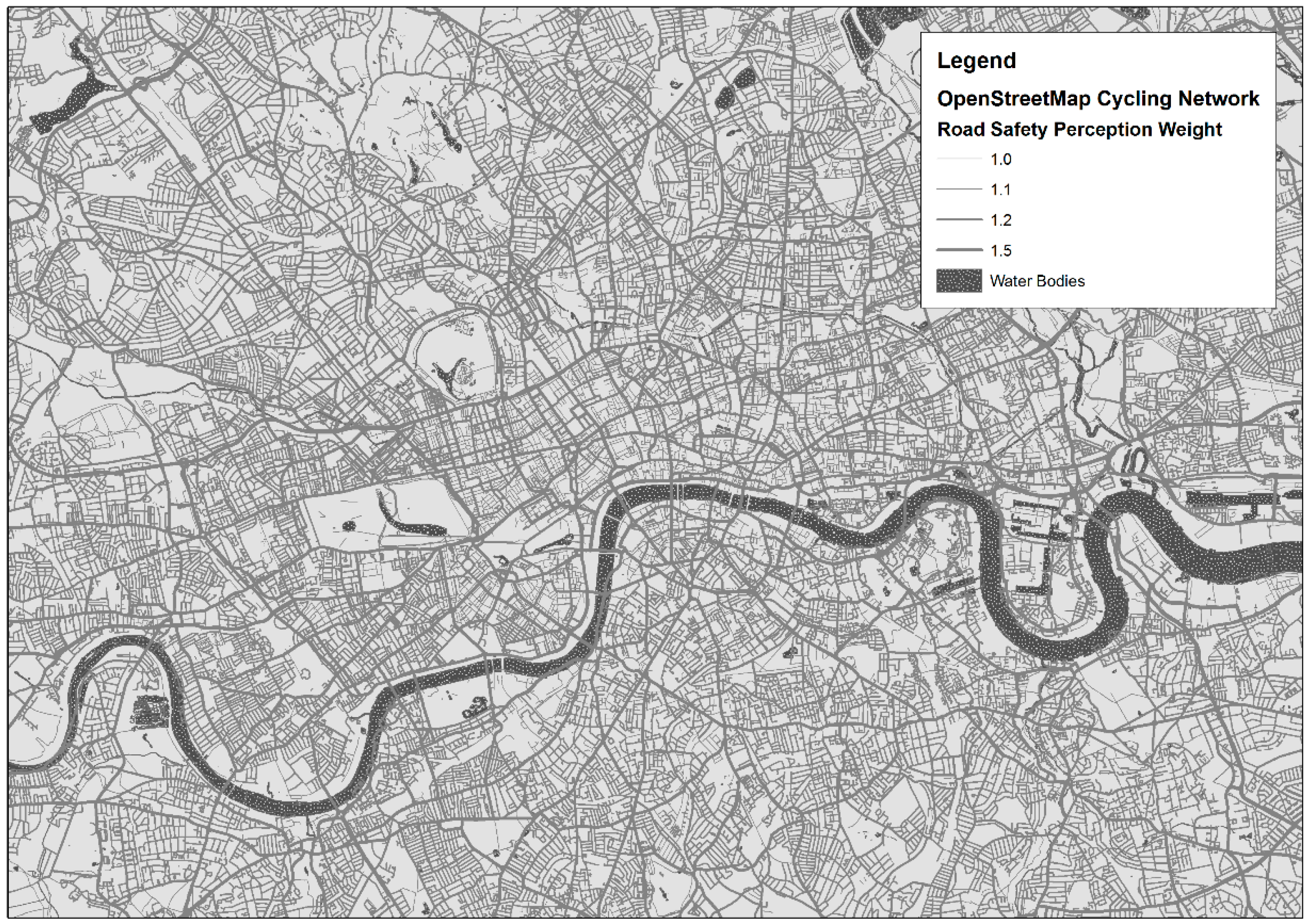
| VSafe | One of the largest disincentives to cycling in urban areas is the issue of safety on the road network (especially in London, where cycling infrastructure is patchy and a number of cyclists are killed every year). A weight is therefore applied based on the class of road being traversed. These are assumed weights but can be simply altered to reflect further research on perceptions of risk. | A-Roads, B-Roads: 1.5 times base travel time
Minor roads: 1.2 Residential streets and pedestrian paths: 1.1 Cycle lanes: 1 Adapted from the methodology employed in the CycleStreet route planner [54] |
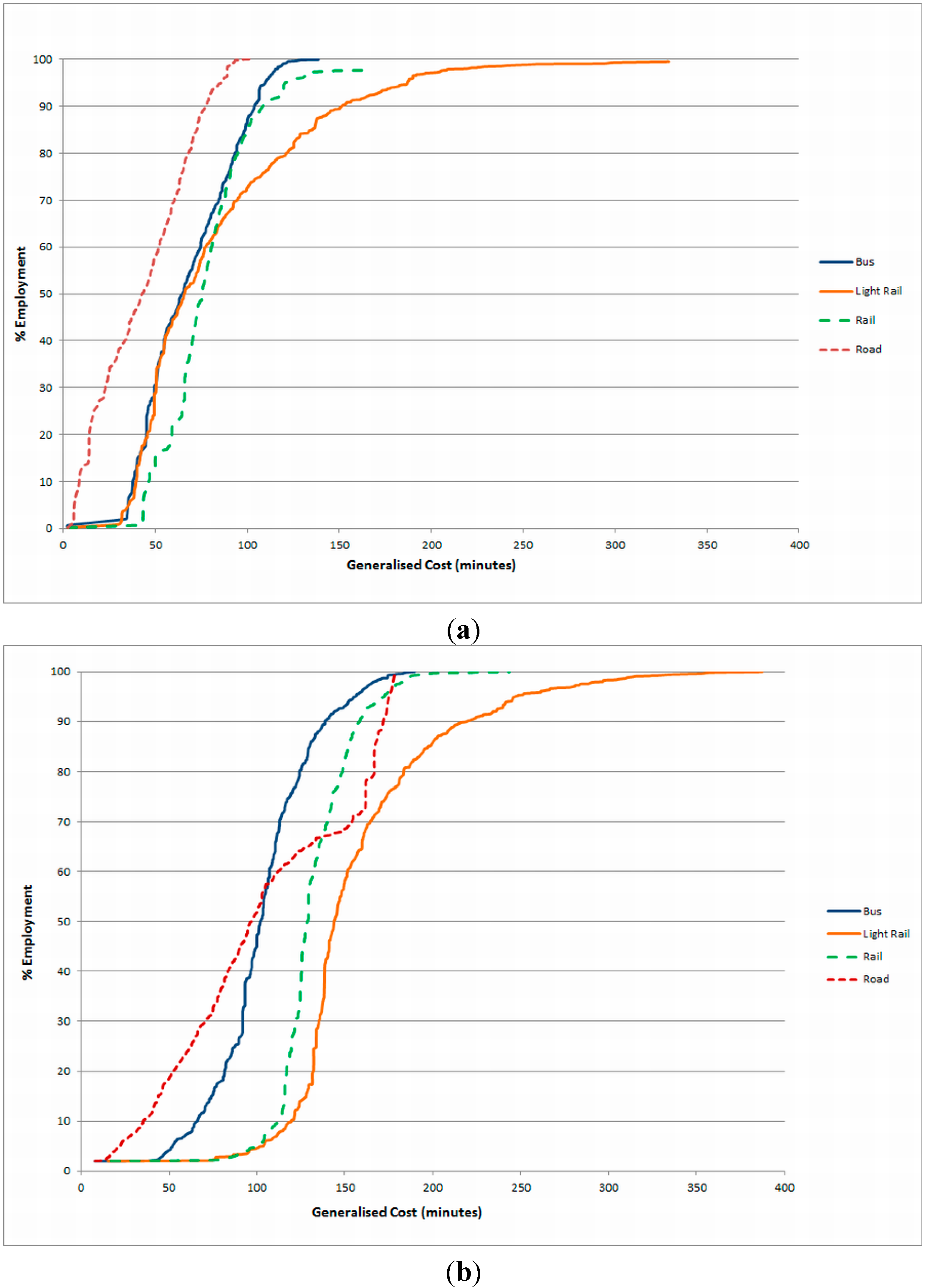
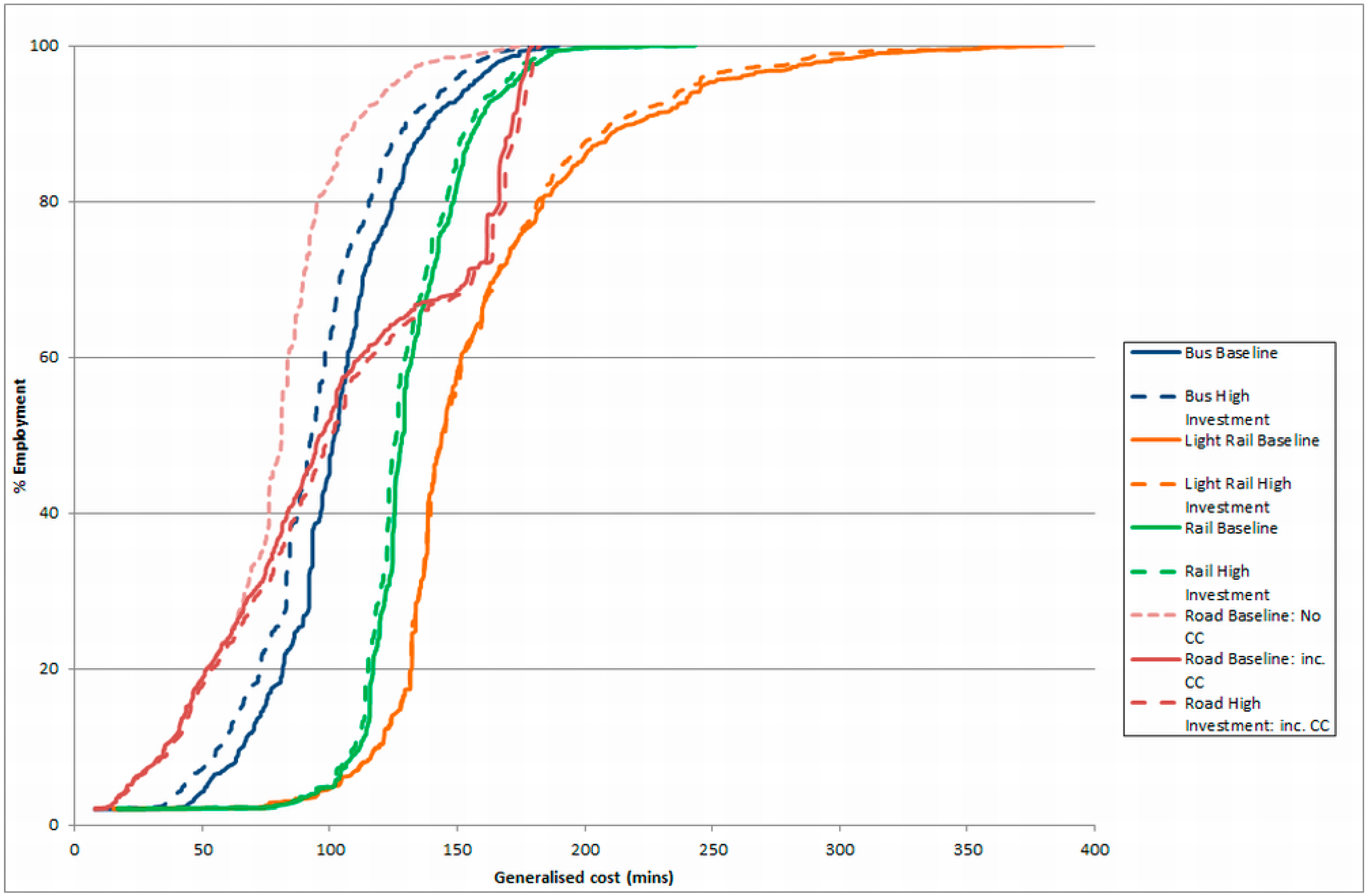
4. Results and Discussion of London Accessibility Study
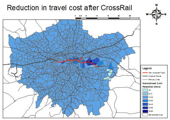
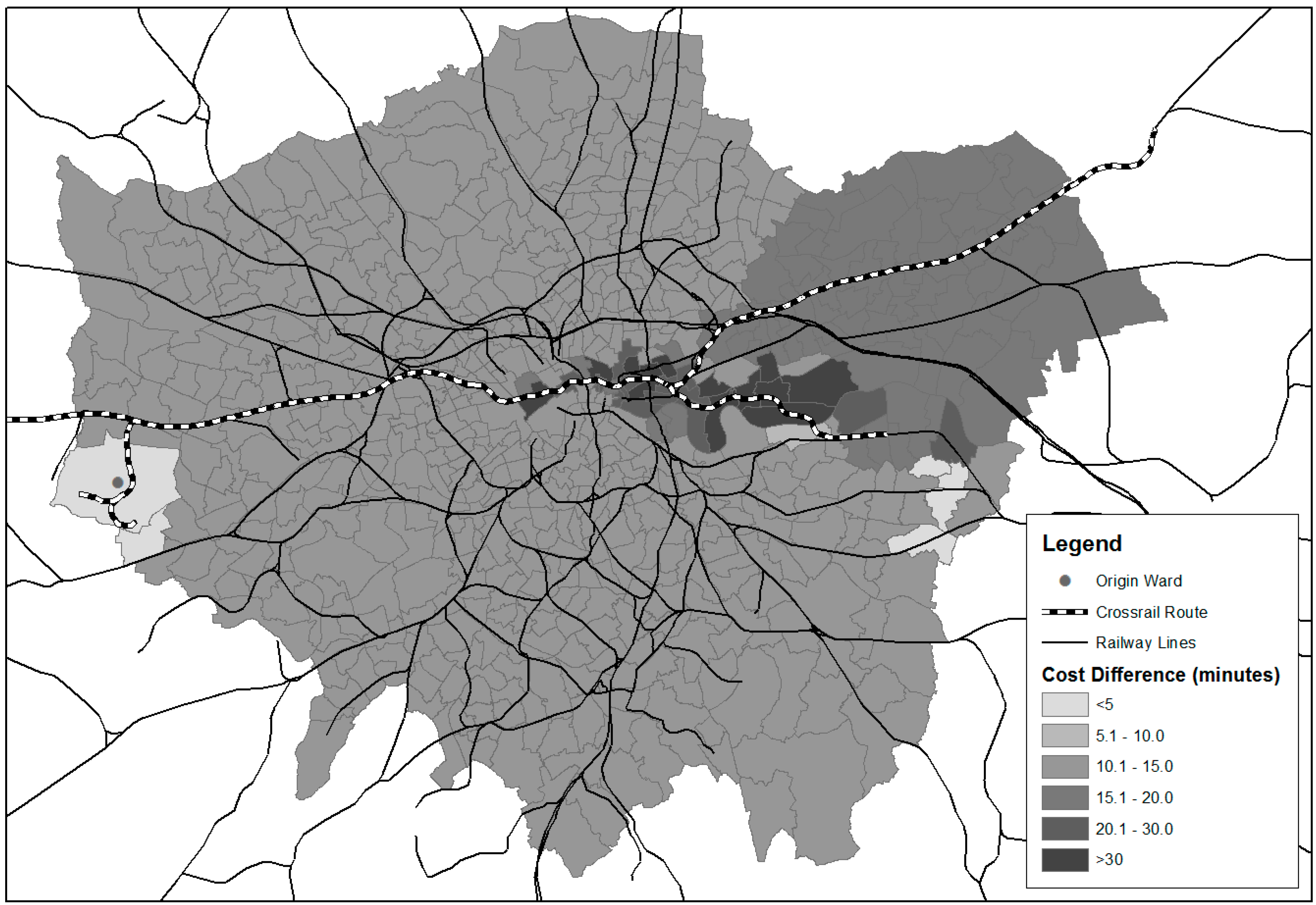
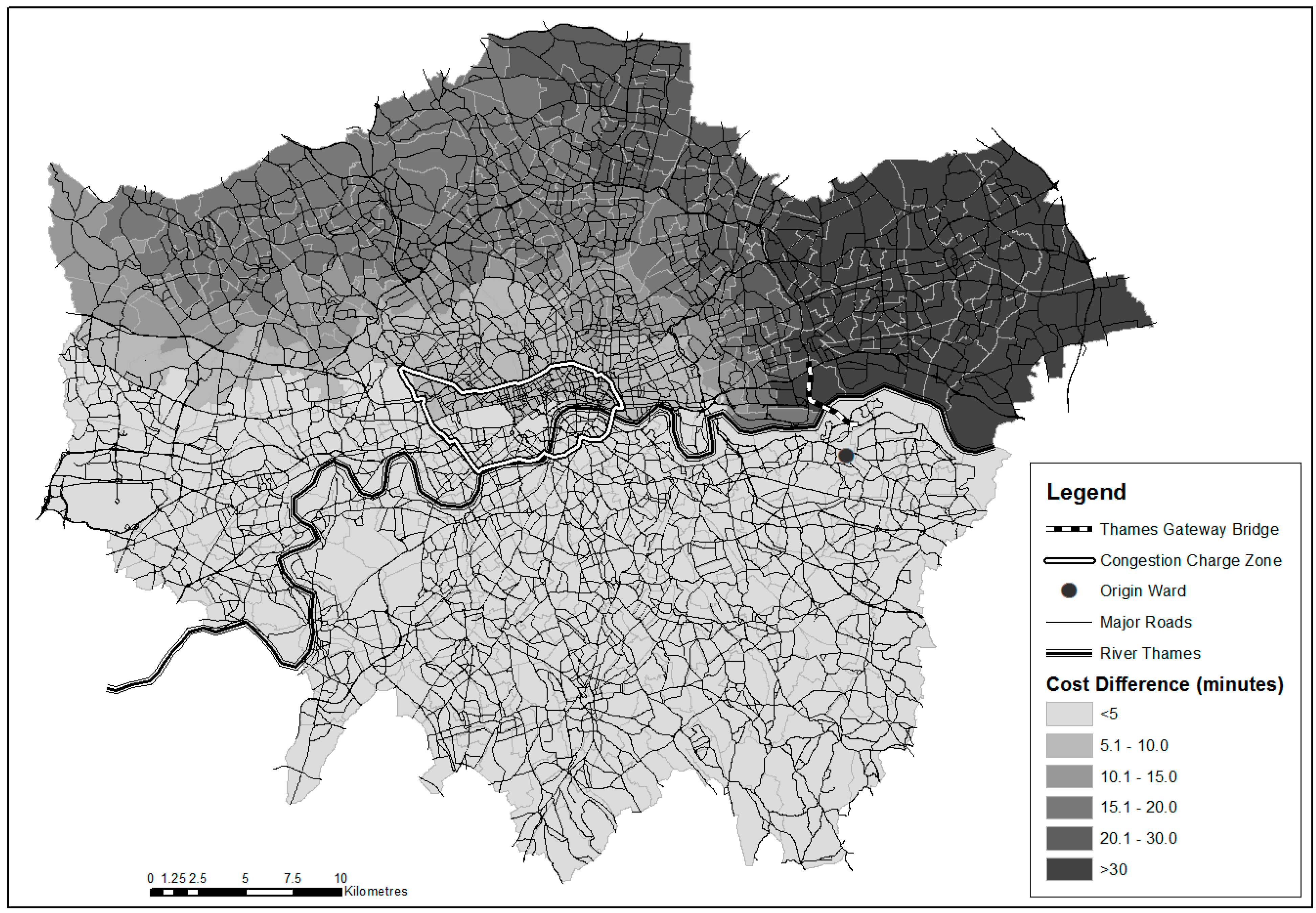
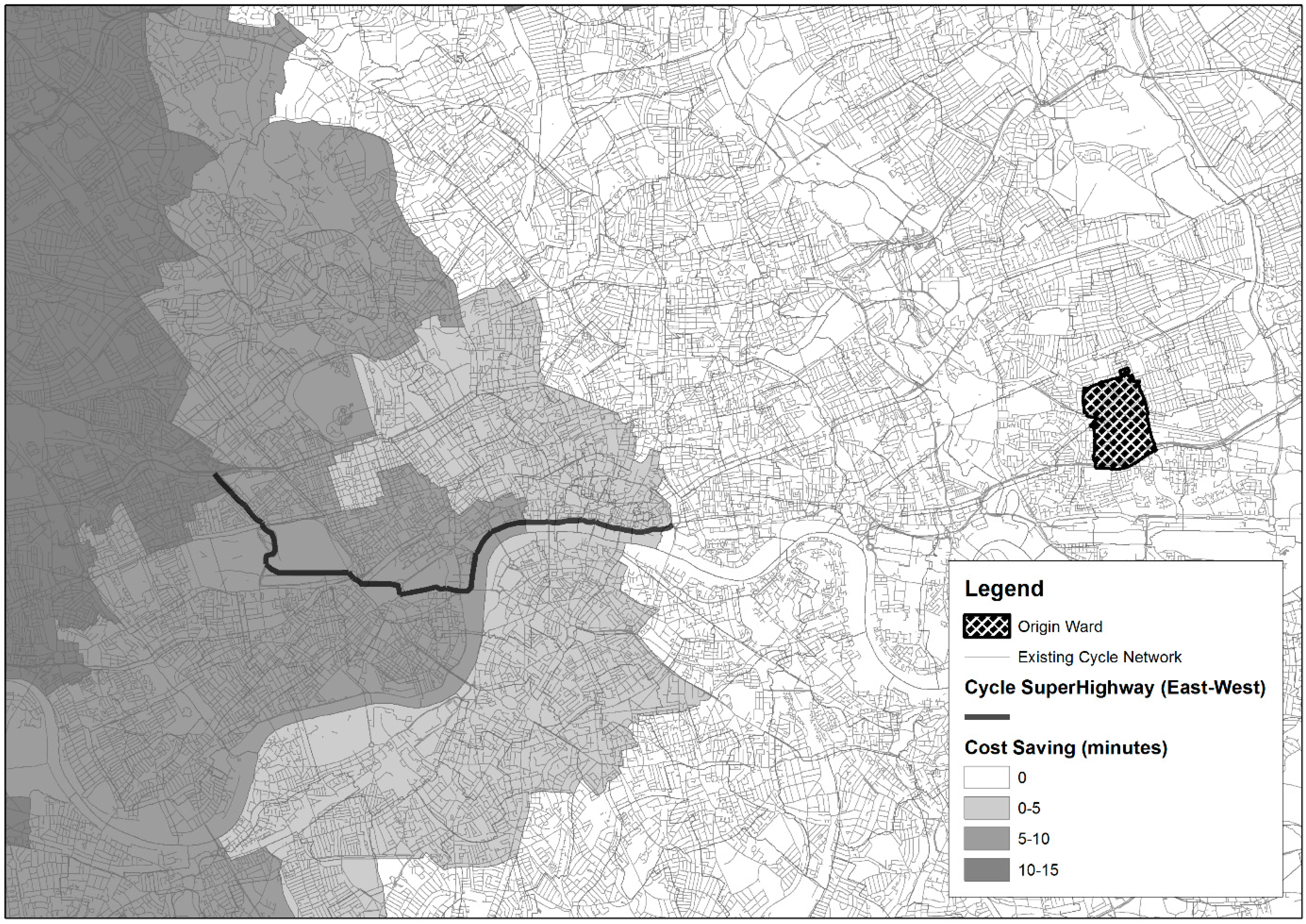
4.1. Testing New Infrastructure Investment


4.2. Accessibility to Employment within London


4.3. Global Accessibility Improvements
| Bus | Light Rail | Rail | Road: With CC | Road: No CC | |
|---|---|---|---|---|---|
| Baseline | 9193 | 13868 | 9767 | 8548 | 6027 |
| Low investment | 9063 (−1.4%) | 13,605 (−1.9%) | 9575 (−2.0%) | 8520 (−0.3%) | 5997 (−0.5%) |
| High investment | 8285 (−9.9%) | 13,325 (−3.9%) | 9490 (−2.8%) | 8698 (+1.7%) | 6176 (−2.5%) |
5. Conclusions
Acknowledgments
Author Contributions
Conflicts of Interest
References
- Pooler, J.A. A family of relaxed spatial interaction models. Prof. Geogr. 1994, 46, 210–217. [Google Scholar] [CrossRef]
- Liu, S.; Zhu, X. An integrated GIS approach to accessibility analysis. Trans. GIS 2004, 8, 45–62. [Google Scholar] [CrossRef]
- Geurs, K.T.; van Wee, B. Accessibility evaluation of land-use and transport strategies: Review and research directions. J. Transp. Geogr. 2004, 12, 127–114. [Google Scholar] [CrossRef]
- Bristow, G.; Farrington, J.; Shaw, J.; Richardson, T. Developing an evaluation framework for crosscutting policy goals: The Accessibility Policy Assessment Tool. Environ. Plan. A 2009, 41, 48–62. [Google Scholar] [CrossRef]
- Hull, A.; Silva, C.; Bertolini, L. Accessibility Instruments for Planning Practice, COST, Brussels; COST: Brussels, Belgium, 2012. Available online: http://www.accessibilityplanning.eu/wp-content/uploads/2012/10/COST-Report-1-FINAL.pdf (accessed on 15 December 2013).
- Van Wee, B. Evaluating the impact of land use on travel behaviour: The environment versus accessibility. J. Transp. Geogr. 2011, 19, 1530–1533. [Google Scholar] [CrossRef]
- Grengs, J. Job accessibility and the modal mismatch in Detroit. J. Transp. Geogr. 2010, 18, 42–54. [Google Scholar] [CrossRef]
- Foth, N.; Manaugh, K.M.; El-Geneidy, A. Towards equitable transit: Examining transit accessibility and social need in Toronto, Canada, 1996–2006. J. Transp. Geogr. 2013, 29, 1–10. [Google Scholar] [CrossRef]
- Rydin, Y. Spatial planning for sustainable urban development. In Governing for Sustainable Urban Development; Earthscan: London, UK, 2010; pp. 107–110. [Google Scholar]
- Hansen, W. How accessibility shapes land use. J. Am. Inst. Plan. 1959, 25, 73–76. [Google Scholar] [CrossRef]
- Lowry, I.S. A Model of Metropolis RM-4035-RC; The Rand Corporation: Santa Monica, CA, USA, 1964. [Google Scholar]
- Levinson, D.M. Accessibility and the journey to work. J. Transp. Geogr. 1998, 6, 11–21. [Google Scholar] [CrossRef]
- Forrester, J.W. Urban Dynamics; MIT Press: Cambridge, MA, USA, 1969. [Google Scholar]
- Wegener, M. Applied models of urban land use, transport and environment: State of the art and future developments. In Network Infrastructure and the Urban Environment. Advances in Spatial Systems Modelling; Lundqvist, L., Mattsson, L.-G., Kim, T.J., Eds.; Springer Verlag: Berlin/Heidelberg, Germany, 1998; pp. 245–267. [Google Scholar]
- Waddell, P. UrbanSim: Modeling urban development for land use, transportation and environmental planning. J. Am. Plan. Assoc. 2002, 68, 297–314. [Google Scholar] [CrossRef]
- Echenique, M.H.; Hargreaves, A.J.; Mitchell, G.; Namdeo, A. Growing cities sustainably: Does urban form really matter? J. Am. Plan. Assoc. 2012, 78, 121–137. [Google Scholar] [CrossRef]
- Clarke, K.C. A decade of cellular urban modeling with SLEUTH: Unresolved issues and problems. In Planning Support Systems for Cities and Regions; Brail, R.K., Ed.; Lincoln Institute of Land Policy: Cambridge, MA, USA, 2008; pp. 47–60. [Google Scholar]
- Batty, M. Building a Science of Cities; UCL Working Papers Series No. 170; University College London: London, UK, November 2012. [Google Scholar]
- Hunt, J.D.; Kriger, D.S.; Miller, E.J. Current operational urban land-use-transport modelling frameworks: A review. Transp. Rev. 2005, 25, 329–376. [Google Scholar] [CrossRef]
- Cooper, S.; Wright, P.; Ball, R. Measuring the accessibility of opportunities and services in dense urban environments: Experiences from London. In Proceedings of the European Transport Conference 2009, Noordwijkerhout, The Netherlands, 5 October 2009.
- Brown, M.; Wood, T. Accession—Accessibility analysis for local transport planning. In Proceedings of the European Transport Conference 2004, Strasbourg, France, 4 October 2004.
- Te Brömmelstroet, M.; Silva, C.; Bertolini, L. COST Action—Assessing Usability of Accessibility Instruments; COST Office: Brussels, Belgium, 2014. [Google Scholar]
- O'Sullivan, D.; Morrison, A.; Shearer, J. Using desktop GIS for the investigation of accessibility by public transport: An isochrone approach. Int. J. Geogr. Inf. Sci. 2000, 14, 85–104. [Google Scholar] [CrossRef]
- Lei, T.L.; Church, R.L. Mapping transit-based access: Integrating GIS, routes and schedules. Int. J. Geogr. Inf. Sci. 2010, 24, 283–304. [Google Scholar] [CrossRef]
- Benenson, I.; Martens, K.; Rofé, Y.; Kwartler, A. Public transport versus private car GIS-based estimation of accessibility applied to the Tel Aviv metropolitan area. Ann. Reg. Sci. 2010, 47, 499–515. [Google Scholar] [CrossRef]
- Mavoa, S.; Witten, K.; McCreanor, T.; O’Sullivan, D. GIS based destination accessibility via public transit and walking in Auckland. J. Transp. Geogr. 2012, 20, 15–22. [Google Scholar] [CrossRef]
- Chen, S.; Claramunt, C.; Ray, C. A spatio-temporal modelling approach for the study of the connectivity and accessibility of the Guangzhou metropolitan network. J. Transp. Geogr. 2014, 36, 12–25. [Google Scholar] [CrossRef]
- Curtis, C.; Scheurer, J. Planning for sustainable accessibility: Developing tools to aid discussion and decision making. Prog. Plan. 2010, 74, 53–106. [Google Scholar] [CrossRef]
- Hall, J.W.; Dawson, R.J.; Walsh, C.L.; Barker, T.; Barr, S.L.; Batty, M.; Bristow, A.L.; Burton, A.; Carney, S.; Dagoumas, A.; et al. Engineering Cities: How Can Cities Grow Whilst Reducing Emissions and Vulnerability? The Tyndall Centre for Climate Change Research: Newcastle, UK, 2009. [Google Scholar]
- Walsh, C.L.; Dawson, R.J.; Hall, J.W.; Barr, S.L.; Batty, M.; Bristow, A.L.; Carney, S.; Dagoumas, A.; Ford, A.; Tight, M.R.; et al. Assessment of climate change mitigation and adaptation in cities. Proc. ICE: Urban Des. Plan. 2011, 164, 75–84. [Google Scholar] [CrossRef]
- Wachs, M.; Kumagi, T.G. Physical accessibility as a social indicator. Soc.-Econ. Plan. Sci. 1973, 7, 437–456. [Google Scholar] [CrossRef]
- Allen, W.B.; Liu, D.; Singer, S. Accessibility measures of U.S. metropolitan areas. Transp. Res. B 1992, 27, 439–449. [Google Scholar] [CrossRef]
- Handy, S.L.; Niemeier, D.A. Measuring accessibility: An exploration of issues and alternatives. Environ. Plan. A 1997, 29, 1175–1194. [Google Scholar] [CrossRef]
- Koenig, J.G. Indicators of urban accessibility: Theory and application. Transportation 1980, 9, 145–172. [Google Scholar] [CrossRef]
- Miller, H.J. Measuring space-time accessibility benefits within transportation networks: Basic theory and computational methods. Geogr. Anal. 1999, 31, 87–212. [Google Scholar]
- Makri, M.C.; Folkesson, C. Accessibility Measures for Analyses of Land Use and Travelling with Geographical Information Systems; Department of Technology and Society, Lund Institute of Technology, Lund University: Lund, Sweden; University & Department of Spatial Planning, University of Karlskrona/Ronneby: Ronneby, Sweden, 1999. [Google Scholar]
- Hillman, R.; Pool, G. GIS-based innovations for modeling public transport accessibility. Traffic Eng. Control 1997, 38, 554–559. [Google Scholar]
- De Ortuzar, J.D.; Willumsen, L.G. Modelling Transport; John Wiley: New York, NY, USA, 2011. [Google Scholar]
- Grey, A. The generalized cost dilemma. Transportation 1978, 7, 261–280. [Google Scholar] [CrossRef]
- Bruzelius, N.A. Microeconomic theory and generalised cost. Transportation 1981, 10, 233–245. [Google Scholar] [CrossRef]
- WebTAG Transport Analysis Guidance. Available online: http://www.dft.gov.uk/webtag/ (accessed on 30 September 2009).
- Mackie, P.J.; Wadman, M.; Fowkes, A.S.; Whelan, G.; Nellthorp, J.; Bates, J. Values of Travel Time Savings in the UK. Available online: http://www.dft.gov.uk/pgr/economics/rdg/valueoftraveltimesavingsinth3130 (accessed on 16 May 2009).
- Nichols, A.J. Standard Generalised Cost Parameters for Modelling Inter-Urban Traffic and Evaluating Inter-Urban Road Schemes, Note 255; Department of the Environment, Mathematical Advisory Unit: London, UK, 1975. [Google Scholar]
- Hopkinson, P.; Wardman, M. Evaluating the demand for new cycle facilities. Transp. Policy 1996, 3, 241–249. [Google Scholar] [CrossRef]
- Noland, R.B.; Kunreuther, H. Short-run and long-run policies for increasing bicycle transportation for daily commuter trips. Transp. Policy 1995, 2, 67–79. [Google Scholar] [CrossRef]
- Rodrıguez, D.A.; Joo, J. The relationship between non-motorized mode choice and the local physical environment. Transp. Res. Part D: Transp. Environ. 2004, 9, 151–173. [Google Scholar] [CrossRef]
- Dijkstra, E.W. A note on two problems in connexion with graphs. Numer. Math. 1959, 1, 269–271. [Google Scholar] [CrossRef]
- ESRI. Network Analyst Documentation. Available online: http://www.esri.com/software/arcgis/extensions/networkanalyst/index.html (accessed on 16 May 2009).
- Feldman, O.; Simmonds, D.; Zachariadis, V.; Mackett, R.; Bosredon, M.; Richmond, E.; Nicoll, J. SIMDELTA—A microsimulation approach to household location modelling. In Proceedings of the World Conference on Transport Research 2007, University of California, Berkeley, CA, USA, 24–28 June 2007.
- National Highway Traffic Safety Administration and the Bureau of Transportation Statistics National Survey of Pedestrian and Bicyclist Attitudes and Behaviors. Available online: http://www.nhtsa.gov/DOT/NHTSA/Traffic%20Injury%20Control/Articles/Associated%20Files/810971.pdf (accessed on 2 January 2014).
- TFL. Transport 2025—Transport Vision for a Growing World City; TfL Group Transport and Planning Policy: London, UK, 2006. [Google Scholar]
- TFL. London Travel Report; Transport for London: London, UK, 2006; p. 40. [Google Scholar]
- TFL. London Congestion Charge Information; Transport for London: London, UK. Available online: http://www.tfl.gov.uk/roadusers/congestioncharging/6709.aspx (accessed on 12 December 2013).
- Cyclestreets Journey Planner, How It Works. Cyclestreets.net. Available online: http://www.cyclestreets.net/journey/help/howitworks/ (accessed on 25 November 2014).
- Crossrail Route Maps. Available online: http://www.crossrail.co.uk/route/maps/route-map (accessed on 29 October 2014).
- TFL. Citizen Hub Consultation on East-West Cycle Superhighway. Available online: https://consultations.tfl.gov.uk/cycling/eastwest (accessed on 22 October 2014).
- Travel in London, Report 6. p. 124. Available online: https://www.tfl.gov.uk/cdn/static/cms/documents/travel-in-london-report-6.pdf (accessed on 20 October 2014).
- GLA. The London Plan: Spatial Development Strategy for Greater London; Greater London Authority: London, UK, 2011. [Google Scholar]
- ONS Nomis Annual Business Inquiry Dataset. Available online: http://www.nomisweb.co.uk (accessed on 14 January 2010).
- DfT. National Travel Survey 2012: Statistical Release; UK Department for Transport: London, UK. Available online: https://www.gov.uk/government/uploads/system/uploads/attachment_data/file/243957/nts2012-01.pdf (accessed on 10 October 2014).
- ONS National Projections: UK Population to Exceed 65 m by 2018. In Office for National Statistics. Available online: http://www.ons.gov.uk/ons/dcp171780_229187.pdf (accessed on 5 December 2013).
- Farrington, J.; Farrington, C. Rural accessibility, social inclusion and social justice: Towards conceptualisation. J. Transp. Geogr. 2005, 13, 1–12. [Google Scholar] [CrossRef]
- Dawson, R.J.; Ball, T.; Werritty, J.; Werritty, A.; Hall, J.W.; Roche, N. Assessing the effectiveness of non-structural flood management measures in the Thames Estuary under conditions of socio-economic and environmental change. Glob. Environ. Chang. 2011, 21, 628–646. [Google Scholar] [CrossRef]
© 2015 by the authors; licensee MDPI, Basel, Switzerland. This article is an open access article distributed under the terms and conditions of the Creative Commons Attribution license (http://creativecommons.org/licenses/by/4.0/).
Share and Cite
Ford, A.C.; Barr, S.L.; Dawson, R.J.; James, P. Transport Accessibility Analysis Using GIS: Assessing Sustainable Transport in London. ISPRS Int. J. Geo-Inf. 2015, 4, 124-149. https://doi.org/10.3390/ijgi4010124
Ford AC, Barr SL, Dawson RJ, James P. Transport Accessibility Analysis Using GIS: Assessing Sustainable Transport in London. ISPRS International Journal of Geo-Information. 2015; 4(1):124-149. https://doi.org/10.3390/ijgi4010124
Chicago/Turabian StyleFord, Alistair C., Stuart L. Barr, Richard J. Dawson, and Philip James. 2015. "Transport Accessibility Analysis Using GIS: Assessing Sustainable Transport in London" ISPRS International Journal of Geo-Information 4, no. 1: 124-149. https://doi.org/10.3390/ijgi4010124