Road Intersection Detection through Finding Common Sub-Tracks between Pairwise GNSS Traces

imec-IPI-UGent, Ghent University, Sint-Pietersnieuwstraat 41, 9000 Ghent, Belgium
*
Author to whom correspondence should be addressed.
ISPRS Int. J. Geo-Inf. 2017, 6(10), 311; https://doi.org/10.3390/ijgi6100311
Submission received: 8 September 2017
/
Revised: 27 September 2017
/
Accepted: 16 October 2017
/
Published: 18 October 2017
Abstract
:This paper proposes a novel approach to detect road intersections from GNSS traces. Different from the existing methods of detecting intersections directly from the road users’ turning behaviors, the proposed method detects intersections indirectly from common sub-tracks shared by different traces. We first compute the local distance matrix for each pair of traces. Second, we apply image processing techniques to find all “sub-paths” in the matrix, which represents good alignment between local common sub-tracks. Lastly, we identify the intersections from the endpoints of the common sub-tracks through Kernel Density Estimation (KDE). Experimental results show that the proposed method outperforms the traditional turning point-based methods in terms of the F-score, and our previous connecting point-based method in terms of computational efficiency.
1. Introduction
Automatic road map generation plays an important role in vehicle navigation systems [1,2,3,4,5], intelligent traffic control [6,7,8,9,10], urban planning [11,12], etc. In particular, the intersections in the road network provide very useful information, such as connectivity, topology and allowable moving direction [13,14,15]. Detecting intersections before road map generation benefits building the topology of the road network.
With the advancement of Global Navigation Satellite System (GNSS) technology in the last few decades, it has been used ubiquitously, such as in mobile phones, wearables, watches, navigation systems, etc. This generates enormous GNSS-derived trace data from a variety of road users. A GNSS trace is a sequence of points with geographic coordinates (latitude, longitude) and timestamps, collected along the route the traveler traverses. Figure 1a shows two GNSS traces on the map. Automatic road map generation aims to infer the road network utilizing these GNSS traces and other information obtained from them, such as moving speed and heading direction.
In literature, most researchers define an intersection as a location or an area where road users may change their moving directions, and detect the intersections by analyzing the road users’ turning behaviors. Karagiorgou and Pfoser used a speed threshold in combination with a change in direction to detect the turn samples from GNSS traces [7]. An agglomerative hierarchical clustering method and a distance threshold were applied to cluster the turn samples into intersection nodes. Wu et al. started with finding the turning points from coarse-gained GNSS traces [16]. The intersecting points were gathered to improve the concentration of the turning points. They then applied the X-means algorithm to cluster the converging points into intersections [17]. Wang et al. detected conflict points, which were defined as locations where two or more traces cross, diverge or converge, and computed the spatial position and boundary circle of each road intersection from the conflict points [18]. In our previous work [19], we also collected and clustered the turning points into intersections. However, we checked the turn types at the turning points to remove mis-detected bends.
Although these researchers applied different algorithms to cluster the turning points into intersections, all of them detected the turning points through thresholding the road users’ moving direction. However, it is difficult to determine an appropriate threshold, especially considering the fluctuations of moving direction.
Different from the methods mentioned above, Fathi and Krumm designed a localized shape descriptor to represent the distribution of GNSS traces around a point [20]. A classifier was trained over the shape descriptors on ground truth data, and later used to discriminate intersection points from non-intersection points. This supervised method requests ground truth training samples and high-sampling-rate traces, which is not suitable for automatic intersection identification.
In our previous work [21], we defined an intersection by its own property as a location connecting three or more road segments in different directions. Based on this definition, we applied the Longest Common SubSequence (LCSS) algorithm to find the common sub-tracks between pairwise GNSS traces, which represent the shared road segment. We collected the endpoints of the common sub-tracks and identified the intersections from the endpoints through Kernel Density Estimation (KDE). Using this method, we achieved higher detection accuracy than the traditional turning point-based method. However, LCSS could only find common sub-tracks in the same moving direction. We had to reverse one of the traces and repeat the whole procedure to identify the common sub-tracks in opposite directions, which increased the computational cost.
In this work, we propose detecting intersections under the same definition of connecting three or more road segments, but employing image processing techniques to find all common sub-tracks without reversing any of the traces. First, we compute and binarize the local distance matrix of pairwise traces. Second, we skeletonize the binary matrix and detect the local “sub-paths”, which represent good alignment between local common sub-tracks. Finally, we identify the intersections from the endpoints of the common sub-tracks through KDE, the same as in our previous method [21].
The remainder of this paper is organized as follows. In the next section, we introduce the problem of detecting intersections through common sub-tracks. Section 3 describes how we detect the common sub-tracks between pairwise traces using image processing techniques, and how we detect the intersections from the endpoints of the common sub-tracks. We show our experimental results in Section 4 and present conclusions in the final section.
2. Problem Statement
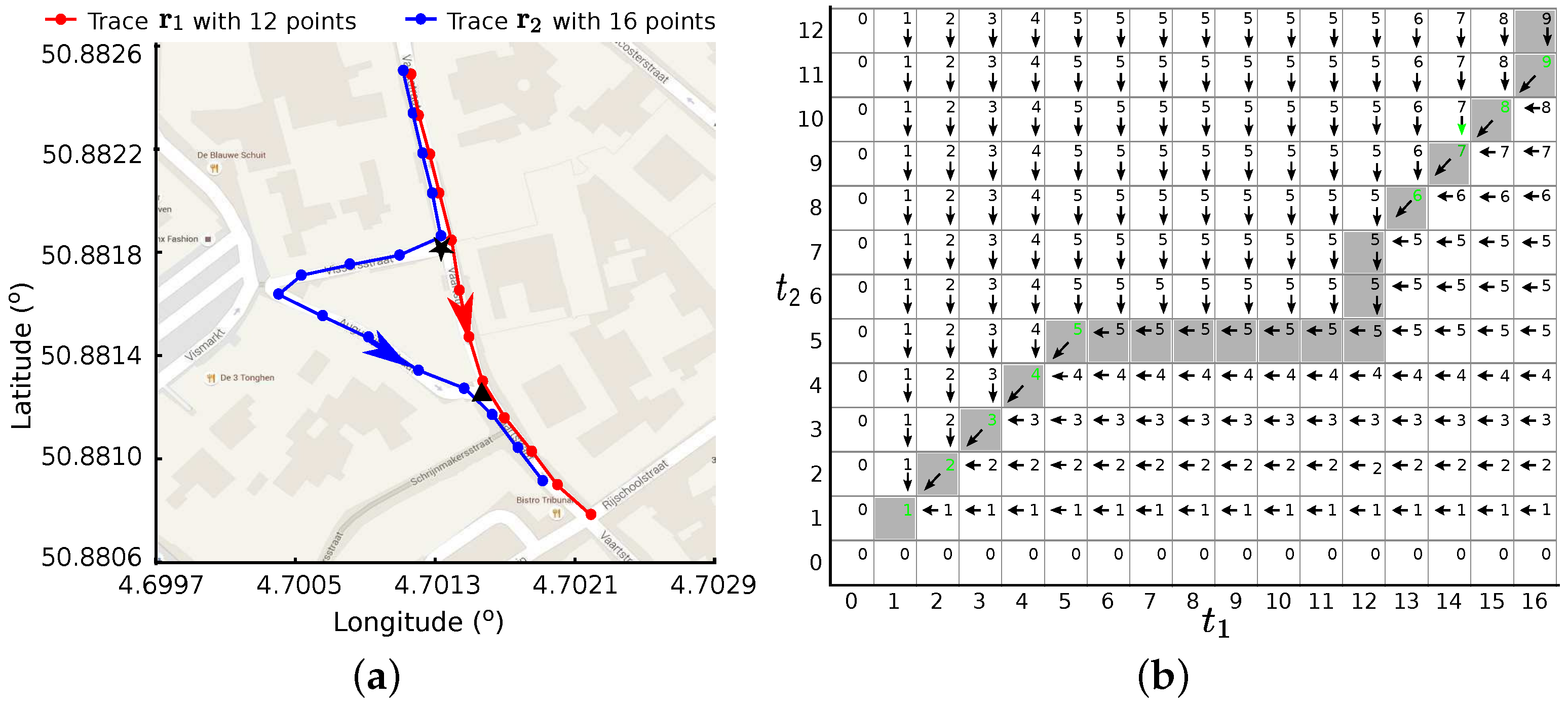
An intersection connects three or more road segments in different directions. At the intersection, road users may merge to the same road segment from other different road segments, or split to other different road segments from the same one. In both scenarios, the road users share one road segment during their journeys, resulting in two GNSS track pieces on this road segment. One end of each track piece is located at this intersection. Therefore, road intersections can be detected through finding the common sub-tracks of the GNSS traces generated in different journeys. Figure 1a shows an example of two GNSS traces with common sub-tracks. The traces are shown in different colors separately with the arrows indicating the moving direction of the road users in their journeys. They first diverge at one intersection indicated using a black star, then converge at another intersection indicated using a black triangle, resulting in two pairs of common sub-tracks: one with five points before the star intersection, and the other one with four points after the triangle intersection.
In our previous work, we applied a dynamic programming technique to find the longest common subsequences [21]. A two-dimensional (2D) length matrix and a direction matrix were first created based on the distance of the points in the GNSS traces. The longest common subsequences were deduced by following the arrows backward through the matrices, i.e., the minimal local distance between the points. Figure 1b shows the LCSS procedure for the two traces in Figure 1a. The optimal path was found by following the arrows directionally from the top-right corner (the ending points of two traces) to the bottom-left corner (the starting points of two traces).
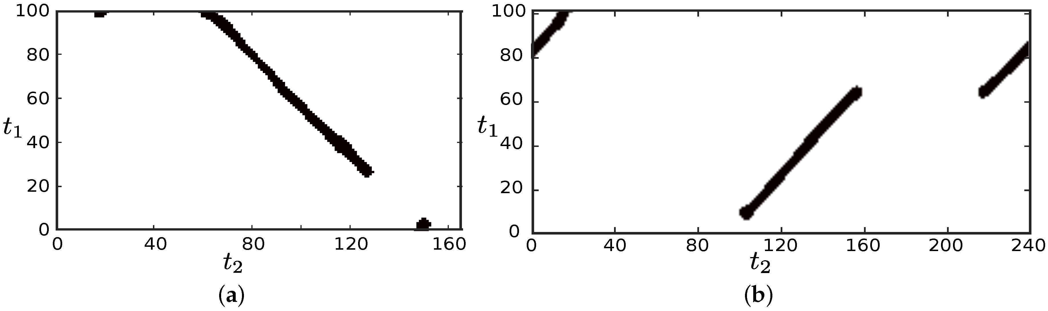
Because of the directional path finding, our previous method could only detect the common sub-tracks in the same moving direction; however, the sub-tracks in opposite directions were ignored. An example is shown in Figure 2a. In the red trace , the road user moves from a higher-longitude region (right on the figure) to a lower-longitude region (left on the figure). In the blue trace , the road user travels through the same road segment in the opposite direction from left to right on the figure. The local distance matrix between the points in the two traces is shown in Figure 2b. By following the minimal local distance from the top-right corner to the left-bottom corner in the matrix, no common sub-tracks will be detected. In our previous work, we reversed one of the GNSS traces and implemented the same dynamic programming again, so as to find these common sub-tracks in opposite directions. This doubled the computational cost.
Another drawback of applying dynamic programming in the finding LCSSs is that the optimal path is deduced through the matrix directionally from one corner to its opposite (or diagonal) corner, which may ignore some local correspondences represented by sub-paths at the other two corners. An example is shown in Figure 2c. In the red trace , the road user simply moves to the right and then down on the figure. In the blue trace , the road user starts at around (41.8674–87.656), moves down to the bottom of the figure, turns to the left of the figure, moves up then right, moves down then diverges to another road, and eventually moves down back to the same road where he or she started. The two traces overlapped three times: the beginning of the blue trace with the ending of the red trace; the beginning of the red trace with the middle of the blue trace; and the ending of the blue trace with the middle of the red traces.
Figure 2d shows three sub-paths for these three pairs of common sub-tracks individually. However, only two of them are detected using an LCSS approach by following the optimal path from the top-right corner to the bottom-left corner in the matrix. The sub-path, which is locates at the top-left corner, fails to be part of the optimal path. These missing local sub-tracks may lead to some of the road intersections undetected.
In this paper, we aim to detect the common sub-tracks through finding all sub-paths in the local distance matrix, instead of only the sub-paths close to the antidiagonal of the matrix as described in our previous method [21].
3. Proposed Method
Figure 3 presents an overview of our approach. We first find the common sub-tracks using image processing techniques on the local distance matrix. The starting and ending points of the common sub-tracks are examined and collected as connecting points. We then apply Kernel Density Estimation (KDE) on the connecting points to detect the road intersections, and remove intersections with low reliability.
3.1. Find Common Sub-Tracks
The proposed method to find the common sub-tracks is presented in dotted box in Figure 3: firstly, compute and binarize the local distance matrix, secondly, skeletonize the binary matrix; finally, detect edges from the skeletons. Only 1-pixel wide edges satisfying the following constraints, which are called “sub-paths” in this paper, represent good alignment between common sub-tracks:
- Length: The edge should not be too short. This prevents point matching between noises in the GNSS data, which deviate from the true path. These noises could originate from various sources, such as vehicle ignition system, motor, atmospheric disturbance, building reflection, etc.
- Monotonicity: The edge may not be straight; but should not bend back on itself. This prevents the temporally distant points in one track from matching the same point in the other track.
- Continuity: The edge should be consecutive. This guarantees that the alignment does not omit any point of either sub-track.
- Slope: The edge should not be too steep or too shallow. This prevents short sub-tracks from matching sub-tracks that are too long.
3.1.1. Binarize the Local Distance Matrix
We first create the local distance matrix for each pair of GNSS traces. Suppose we have two GNSS traces with data points and with , where and are geographical coordinates in latitude and longitude, and and are real local time in DateTime format of “YYYY-MM-DD-HH-MM-SS”. The numbers of samples and need not be the same. The two-dimensional local distance matrix is computed using the spherical law of cosines formula. The value at each cell, , is the geographical distance between point in the first trace and point in the second trace:
where R is The Earth’s radius.
We then apply a thresholding method on the local distance matrix to create a two-dimensional binary matrix . If the geographical distance between point and point , , is less than predefined threshold , is set to 1; otherwise, it is set to 0. The distance threshold should be chosen based on the road width and the expected GNSS error:
Figure 4 shows the binarized distance matrix for Examples 2 and 3, respectively. Every edge, shown in black connected pixels, represents a pair of common sub-tracks. The width of the edge is unfixed, depending on the number of the cells with local distance less than . Therefore, these edges can only establish rough point associations between the common sub-tracks. To get temporally linear alignment between the sub-tracks, we will extract the skeletons of the binarized distance matrix at the next step.
3.1.2. Skeletonize the Local Distance Matrix
We first apply the Zhang–Suen thinning algorithm on the binarized distance matrix to obtain the skeletons [22]. This is an iterative procedure, and each iteration undergoes two sub-iterations:
- Sub-iteration 1. The black pixel is set to white if it satisfies all the following conditions:
- (1)
- The number of 0–1 patterns in the ordered set is 1, where are the eight adjacent pixels of in a window, as shown in Table 1.
- (2)
- It has at least two and not more than six nonzero neighbors.
- (3)
- At least one of the three pixels is 0 (white), i.e., .
- (4)
- At least one of the three pixels is 0 (white), i.e., .
- Sub-iteration 2 is the same as Sub-iteration 1, but with conditions and changed:
- (3’)
- At least one of the three pixels is 0 (white), i.e., .
- (4’)
- At least one of the three pixels is 0 (white), i.e., .
The iteration stops if no pixel is set to white during either sub-iteration. The output of this step is a skeletonized distance matrix with black pixels representing the skeletons. The skeletons of Examples 2 and 3 are shown in Figure 5.
Connected-component labeling techniques could be used to extract the consecutive edges [23]. However, these consecutive edges cannot be used to represent the point associations between the sub-tracks for the following reasons: (a) the Zhang–Suen thinning algorithm itself does not guarantee that the skeleton edge is 1-pixel wide; (b) small spurious branches are detected at the ends of skeleton edges, as shown in red circles in Figure 5. This violates the “Monotonicity” constraint; (c) whether the edges satisfy the “Slope” constraint is still unknown. In the next step, we will propose a new algorithm to extract the “sub-paths” from the skeletons, which can represent good alignment between local sub-tracks.
3.1.3. Detect “Sub-Paths” from the Skeletonized Matrix
The “sub-paths” can be deduced as followed, given the local distance matrix and the skeletonized distance matrix . At first, we search the skeletonized distance matrix and get a nonzero element . This search is conducted in the order of first by the row then by the column . This guarantees no nonzero element with smaller row index . Therefore, the “sub-path” , which starts at the pixel , i.e., , will have to go increasingly along . In other words, only five of eight neighbor pixels with gray background as shown in Table 1, are considered as as candidate pixels for the next element of the “sub-path”, . Secondly, we narrow the candidate pixels from these five pixels down to skeleton pixels, whose value is 1 in the skeletonized distance matrix . We then choose the candidate pixel with the smalled local distance as the second element of the “sub-path”, . Once one pixel in is added to the “sub-path”, its value is set to 0.
The “sub-path” continues to advance until none of the candidate pixels for the next element are skeleton pixels. Subject to the “Monotonicity” constraint, the “sub-path” should not roll back to itself; therefore, only three of the five neighbor pixels, or will be used as candidate pixels from the first iteration, once the advance direction is confirmed in the first instance.
Finally, we examine whether this “sub-path” satisfies the “Length” and “Slope” constraint through the number of steps in and direction individually, and their ratio as well. In this paper, we choose as the length threshold, and as the slope threshold, i.e., .
We then find a new nonzero element in the keletonized distance matrix , and repeat the whole procedure elaborated above to detect more “sub-paths”, until all pixels in the skeletonized distance matrix are set to 0, i.e., .
The outputs of this step are “sub-paths” representing good alignment between common sub-tracks, , , and the common sub-tracks warped along the “sub-paths” and , , with points associated at the same time index .
As shown in Figure 6, one “sub-path” is deduced for Example 2, indicating one pair of common sub-tracks found in the GNSS traces shown in Figure 2a; three “sub-paths” are deduced for Example 3, representing three pairs of common sub-tracks in the GNSS traces shown in Figure 2c. The proposed method successfully detects all common sub-tracks in both scenarios and removes the splitting branches at the ends of the “sub-paths” shown in Figure 5.
3.2. Extract Intersections
Given a dataset of N GNSS traces, we first find the common sub-tracks between each pair of GNSS traces. We then collect the starting and ending points of the common sub-tracks as connecting points, if they are not the starting and ending points of these two GNSS traces. We then detect the intersections from these connecting points through estimating the density of the connecting points over the area covered by the GNSS traces:
- (1)
- Discretize the area into a 2D grid of cells.
- (2)
- (3)
- Convolve the histogram with a Gaussian smoothing function to approximate the Kernel Density Estimation (KDE).
- (4)
- Find the local maximums on the density map as intersection candidates.
Finally, we examine the patterns of the GNSS traces converging or diverging at each intersection candidate. Suppose there are M GNSS traces involved to produce N connecting points for one intersection candidate. If all of the N connecting points are detected from aligning one trace with each of the other traces, the inferred intersection candidate will be removed because the existence of the road segment represented by this single trace needs to be confirmed with more traces. As shown in Figure 7, one single blue trace splits into a different direction from all other black traces at the same location, producing a large amount of connecting points. An intersection is detected from these connecting points. However, this single trace may be an abnormal trace that deviates from the roads to construction areas because of GNSS errors. Therefore, this intersection may not exist physically.
4. Experimental Results
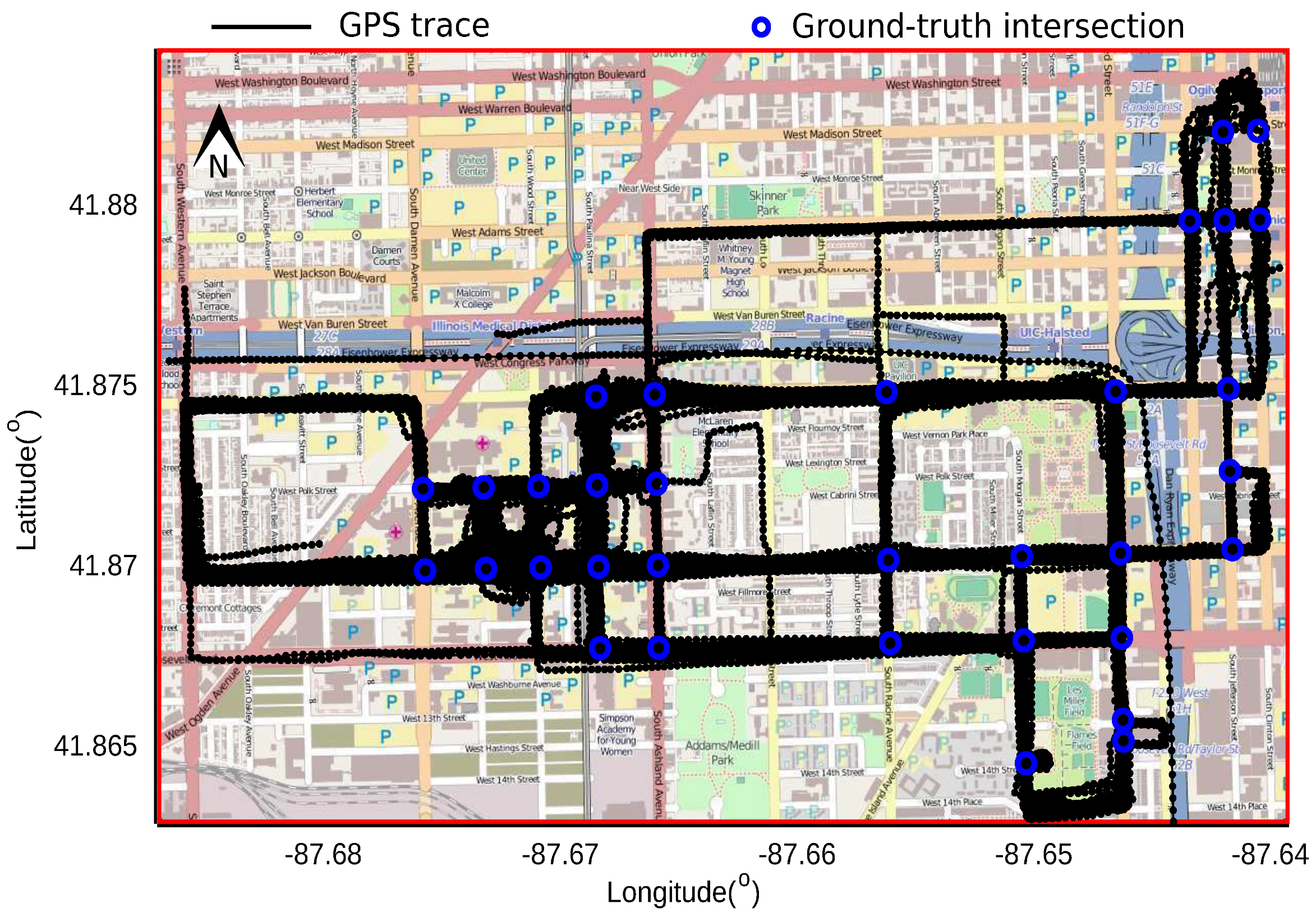
We applied our proposed method on a dataset of campus shuttle traces from the University of Illinois at Chicago (UIC) [25]. This dataset was recorded using the UIC shuttle tracking system, which has an online tracking application that delivers real-time GNSS location information to the server through an iPhone application over the cellular network. This dataset consists of 889 GNSS traces and covers an area of km. The tracking system is designed to send the location at a frequency of every second. However, the actual sampling interval of the recorded traces varies from 1 s to 29 s (average: s and standard deviation: s) because sometimes the server fails to receive the location information. This dataset has a geographic coordinate system, which uses latitude and longitude to describe locations on Earth’s surface. The raw GNSS traces are depicted in black lines in Figure 8. The dots indicate the point locations. To calculate the accuracy of the intersections detected from the shuttle traces, we use OpenStreetMap as the ground truth map. Figure 8 shows 33 ground truth intersections using blue circles, only on the streets that were actually traversed by the shuttles.
4.1. Results of the Proposed Method
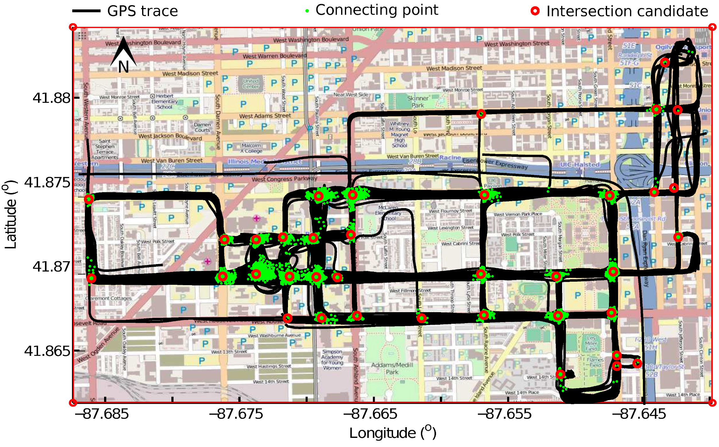
Figure 9 shows the connecting points with green dots, and the intersection candidates with red circles. Most of the connecting points are located at the road intersections, while some of them are on the road segments because of GNSS errors. In total, 37 intersection candidates are extracted from the connecting points through KDE.
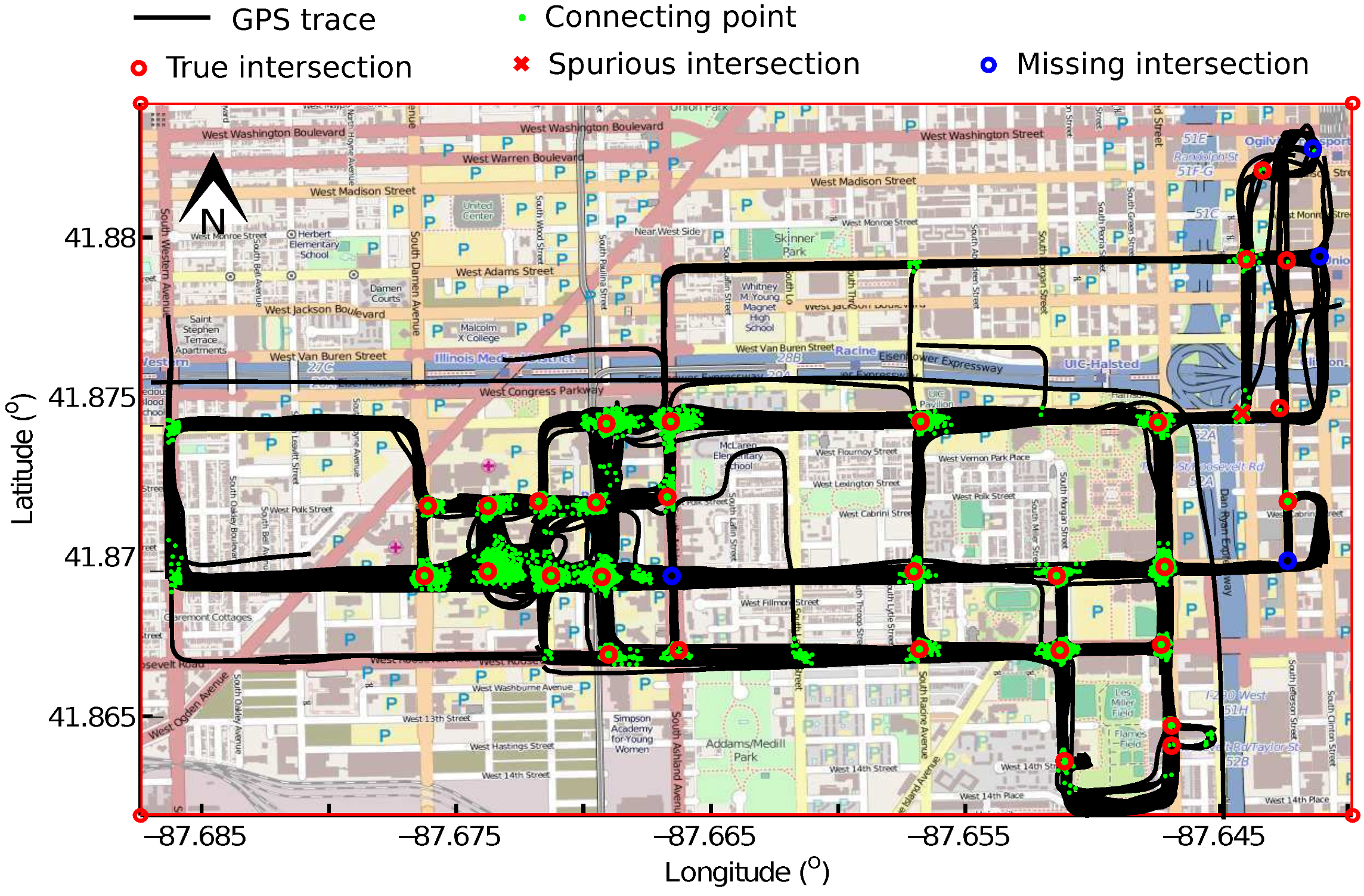
Figure 10 shows the true intersections after checking the patterns of GNSS traces diverging or converging at the intersection candidates. In total, 7 of the 37 candidates are removed, leaving 29 true intersections depicted using red circles and one spurious intersection using a red cross.
This “spurious” intersection is actually a true intersection, but is missing on the ground truth map. This dataset was recorded in April 2011, when all the road segments meeting at this intersection were traversable. However, we downloaded the ground truth map in August 2014, when one of the road segments was blocked because of road construction. Therefore, this location was a “bend” connecting only two road segments on the ground truth map. In order to directly compare with our previous methods [19,21], we did not correct this on the ground truth map, but kept it as a bend instead of an intersection.
4.2. Comparison
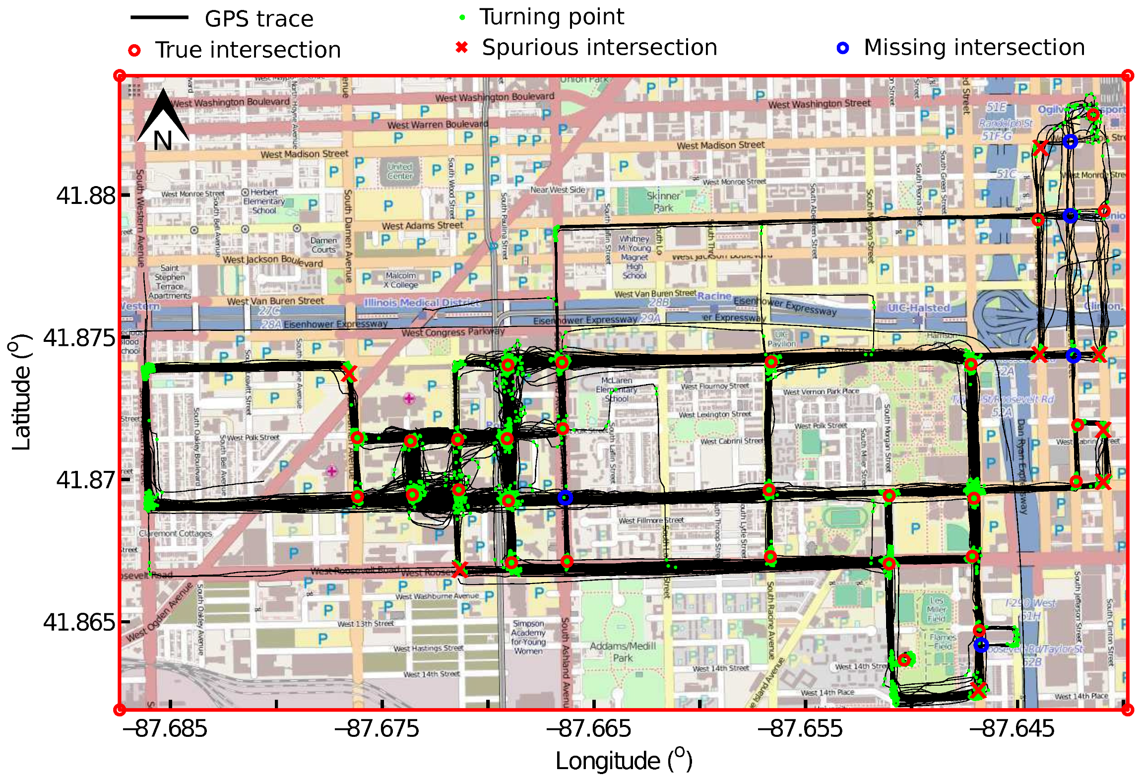
In this section, we compare our proposed method with our two previous methods: one is based on the classical turning points detection [19], and the other is based on connecting points detection using LCSS [21]. Figure 11 and Figure 12 depict the intersections detected using these two methods, respectively.
As shown in Figure 11, thirty-six intersections are detected from the turning points after the bend removal. Twenty-eight of them are true intersections, and eight are spurious intersections that do not exist on the ground truth map. Five of the ground truth intersections are detected unsuccessfully. The true, spurious and missing intersections are indicated using red circles, red crosses and blue circles separately. The average distance between these 28 correctly detected true intersections and their ground truth is m. Figure 8 shows the intersections detected from the connecting points using LCSS. In total, 28 intersections are detected, including 27 true intersections and one spurious intersection. Six of the ground truth intersections are undetected. The average distance between the true intersections and their ground truth is m.
Compared to Figure 11 and Figure 12, our proposed method detects more true intersections and less spurious intersections, as shown in Figure 10. The average distance between the true intersections and their ground truth calculated using our proposed method is m, which is close to that using the previous connecting point-based method ( m), but much smaller than the one using the turning point-based method ( m).
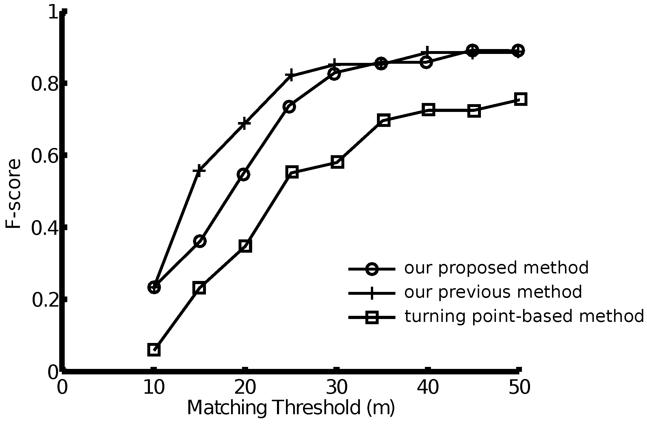
Figure 13 shows the accuracy of the intersections using the well-known F-score [26,27]. The matching threshold is defined as the allowable distance between the geographical location of the detected intersections and their ground truth location on OpenStreetMap. With a matching threshold of 30 m, both of the connecting point-based methods reach an F-score of approximately , outperforming the turning point-based method whose F-score value is only around .
In general, the turning point-based methods are more efficient than the connecting point-based methods because turning point-based methods process each of the GNSS traces in the dataset individually, while connecting point-based methods deal with each pair of the GNSS traces.
Compared to our previous connecting point-based method using LCSS, our proposed method in this paper is almost two times faster because it is unnecessary to reverse one of the pairwise traces to find the common sub-tracks in the opposite direction. For this dataset with 889 GNSS traces, it takes around 50 min to find the connecting points between all pairs of GNSS traces using the LCSS algorithm, and close to 30 min using the proposed method. The computational cost of dealing with all possible pairs of GNSS traces in a data set is enormous, and increases rapidly as the dataset gets bigger. In practice, we randomly pick up a fixed amount of traces with reasonable costs for intersection detection. However, our proposed method outperforms our previous method using LCSS in computational efficiency in either way.
5. Conclusions
We have presented a novel approach to detect intersections through analyzing pairwise GNSS traces. We apply image processing techniques first on the local distance matrix of pairwise traces to find all common sub-tracks between them, which represent the shared road segments traversed in these traces. The starting and ending points of the common sub-tracks are collected as connecting points for intersection identification through KDE. Finally, we confirm the existence of each intersection through examining the connecting points and GNSS traces involved. The main advantage of our proposed method is the intersection accuracy. We detect more true intersections and less spurious intersections compared to the turning point-based method. We also improve the computational efficiency compared to our previous connecting point-based method using LCSS. However, the proposed method is still not efficient enough for huge data sets.
This paper is a good example of applying and merging techniques from different fields, Geographic Information Systems (GIS) and image processing in this case. The proposed method could also be applied to other types of sequence data, such as DNA sequences and financial data.
Acknowledgments
This research was supported by imec, Netherlands under the project EI2. The authors would like to thank BITS laboratory for providing the Chicago dataset.
Author Contributions
The research was conducted by the main author, Xingzhe Xie, under the supervision of the co-author Wilfried Philips.
Conflicts of Interest
The authors declare no conflicts of interest.
References
- Biagioni, J.; Eriksson, J. Inferring Road Maps from Global Positioning System Traces. Transp. Res. Rec. 2012, 2291, 61–71. [Google Scholar] [CrossRef]
- Edelkamp, S.; Schrödl, S. Route planning and map inference with global positioning traces. In Computer Science in Perspective; Springer: Berlin, Germany, 2003; pp. 128–151. [Google Scholar]
- Cao, L.; Krumm, J. From GPS traces to a routable road map. In Proceedings of the 17th ACM SIGSPATIAL International Conference on Advances in Geographic Information Systems, Washington, DC, USA, 4–6 November 2009; pp. 3–12. [Google Scholar]
- Worrall, S.; Nebot, E. Automated process for generating digitised maps through GPS data compression. In Proceedings of the Australasian Conference on Robotics and Automation, Brisbane, Australia, 10–12 December 2007. [Google Scholar]
- Xie, X.; Wong, K.; Aghajan, H.; Philips, W. Smart route recommendations based on historical GPS trajectories and weather information. In Proceedings of the Mobile Ghent, Ghent, Belgium, 23–25 October 2013. [Google Scholar]
- Niehoefer, B.; Burda, R.; Wietfeld, C.; Bauer, F.; Lueert, O. GPS community map generation for enhanced routing methods based on trace-collection by mobile phones. In Proceedings of the 1st International Conference on Advances in Satellite and Space Communications, Colmar, France, 20–25 July 2009; pp. 156–161. [Google Scholar]
- Karagiorgou, S.; Pfoser, D. On vehicle tracking data-based road network generation. In Proceedings of the 20th International Conference on Advances in Geographic Information Systems, Redondo Beach, CA, USA, 7–9 November 2012; pp. 89–98. [Google Scholar]
- Davics, J.; Beresford, A.R.; Hopper, A. Scalable, distributed, real-time map generation. IEEE Pervasive Comput. 2006, 5, 47–54. [Google Scholar]
- Xie, X.; Philips, W.; Veelaert, P.; Aghajan, H. Road network inference from GPS traces using DTW algorithm. In Proceedings of the 17th IEEE International Conference on Intelligent Transportation Systems, Qingdao, China, 8–11 October 2014; pp. 906–911. [Google Scholar]
- Herrera, J.C.; Work, D.B.; Herring, R.; Ban, X.J.; Jacobson, Q.; Bayen, A.M. Evaluation of traffic data obtained via GPS-enabled mobile phones: The Mobile Century field experiment. Transp. Res. Part C 2010, 18, 568–583. [Google Scholar] [CrossRef]
- Szeto, W.Y.; Jiang, Y.; Wang, D.Z.W.; Sumalee, A. A sustainable road network design problem with land use transportation interaction over time. Netw. Spat. Econ. 2015, 15, 791–822. [Google Scholar] [CrossRef] [Green Version]
- Comber, A.; Brunsdon, C.; Green, E. Using a GIS-based network analysis to determine urban greenspace accessibility for different ethnic and religious groups. Landsc. Urban Plan. 2008, 86, 103–114. [Google Scholar] [CrossRef]
- Zheng, Y.; Zhang, L.; Xie, X.; Ma, W.Y. Mining interesting locations and travel sequences from GPS trajectories. In Proceedings of the 18th International Conference on World Wide Web, Madrid, Spain, 20–24 April 2009; pp. 791–800. [Google Scholar]
- You, Q.; Krumm, J. Transit tomography using probabilistic time geography: Planning routes without a road map. J. Locat. Based Serv. 2014, 8, 211–228. [Google Scholar] [CrossRef]
- Xie, X.; Wong, K.; Aghajan, H.; Philips, W. Analyzing cyclists’ behaviors and exploring the environments from cycling tracks. In Proceedings of the Cycling Data Challenge 2013 Workshop, Leuven, Belgium, 14 May 2013. [Google Scholar]
- Wu, J.; Zhu, Y.; Ku, T.; Wang, L. Detecting road intersections from coarse-gained GPS traces based on clustering. J. Comput. 2013, 8, 2959–2965. [Google Scholar] [CrossRef]
- Pelleg, D.; Moore, A.W. X-means: Extending K-means with efficient estimation of the number of clusters. In Proceedings of the Seventeenth International Conference on Machine Learning (ICML ’00), Stanford, CA, USA, 29 June–2 July 2000; pp. 727–734. [Google Scholar]
- Wang, J.; Rui, X.; Song, X.; Tan, X.; Wang, C.; Raghavan, V. A novel approach for generating routable road maps from vehicle GPS traces. Int. J. Geogr. Inf. Sci. 2015, 29, 69–91. [Google Scholar] [CrossRef]
- Xie, X.; Wong, K.; Aghajan, H.; Veelaert, P.; Philips, W. Inferring directed road networks from GPS traces by track alignment. Int. J. Geo-Inf. 2015, 4, 2446–2471. [Google Scholar] [CrossRef] [Green Version]
- Fathi, A.; Krumm, J. Detecting road intersections from GPS traces. In Proceedings of the Geographic Information Science, Zurich, Switzerland, 14–17 September 2010; pp. 56–69. [Google Scholar]
- Xie, X.; Liao, W.; Aghajan, H.; Veelaert, P.; Philips, W. Detecting road intersections from gps traces using longest common subsequence algorithm. Int. J. Geo-Inf. 2016, 6, 1. [Google Scholar] [CrossRef]
- Comber, A.; Brunsdon, C.; Green, E.; Zhang, T.Y.; Suen, C.Y. A fast parallel algorithm for thinning digital patterns. Commun. ACM 1984, 27, 236–239. [Google Scholar]
- Dillencourt, M.B.; Samet, H.; Tamminen, M. A general approach to connected-component labeling for arbitrary image representations. J. ACM 1992, 39, 253–280. [Google Scholar] [CrossRef]
- Scott, D.W. Multivariate Density Estimation: Theory, Practice, and Visualization; John Wiley & Sons: Hoboken, NJ, USA, 2015. [Google Scholar]
- BITS Networked Systems Laboratory. Available online: http://bits.cs.uic.edu/ (accessed on 21 December 2016).
- Yang, Y. An evaluation of statistical approaches to text categorization. Inf. Retr. 1999, 1, 69–90. [Google Scholar] [CrossRef]
- Liu, B. Web Data Mining; Springer: Berlin, Germany, 2007. [Google Scholar]
Figure 1.
An example of two GNSS traces sharing two road segments. (a) two GNSS traces, which diverge at the star intersection from one common road segment onto two different road segments, then converge to another common road segment at the triangle intersection; (b) the length and direction matrices used in the Longest Common SubSequence (LCSS) procedure to find the common sub-tracks.

Figure 2.
Examples of GNSS traces fail to find common sub-tracks using the LCSS method. (a) example 2 of two GNSS traces moving in opposite directions on the same road; (b) the local distance matrix for Example 2; (c) example 3 of two GNSS traces sharing multiple common sub-tracks; (d) the local distance matrix for Example 3.
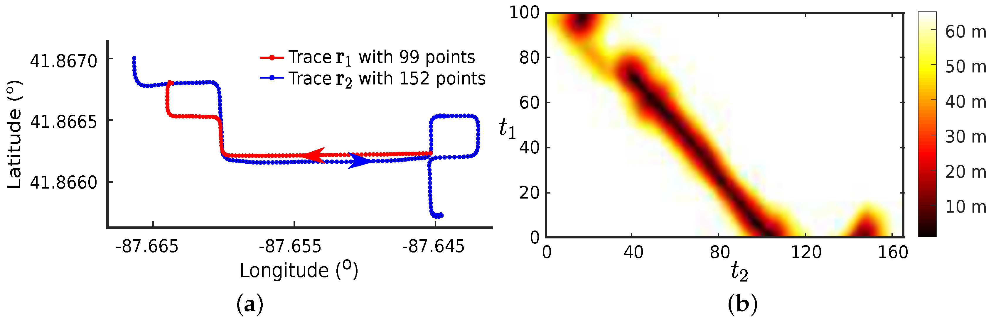
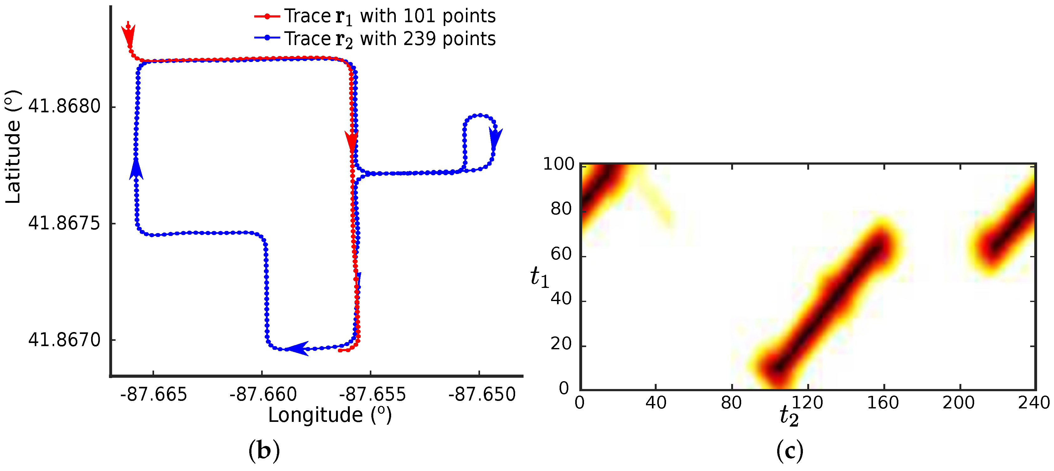
Figure 3.
Overview of the proposed approach.
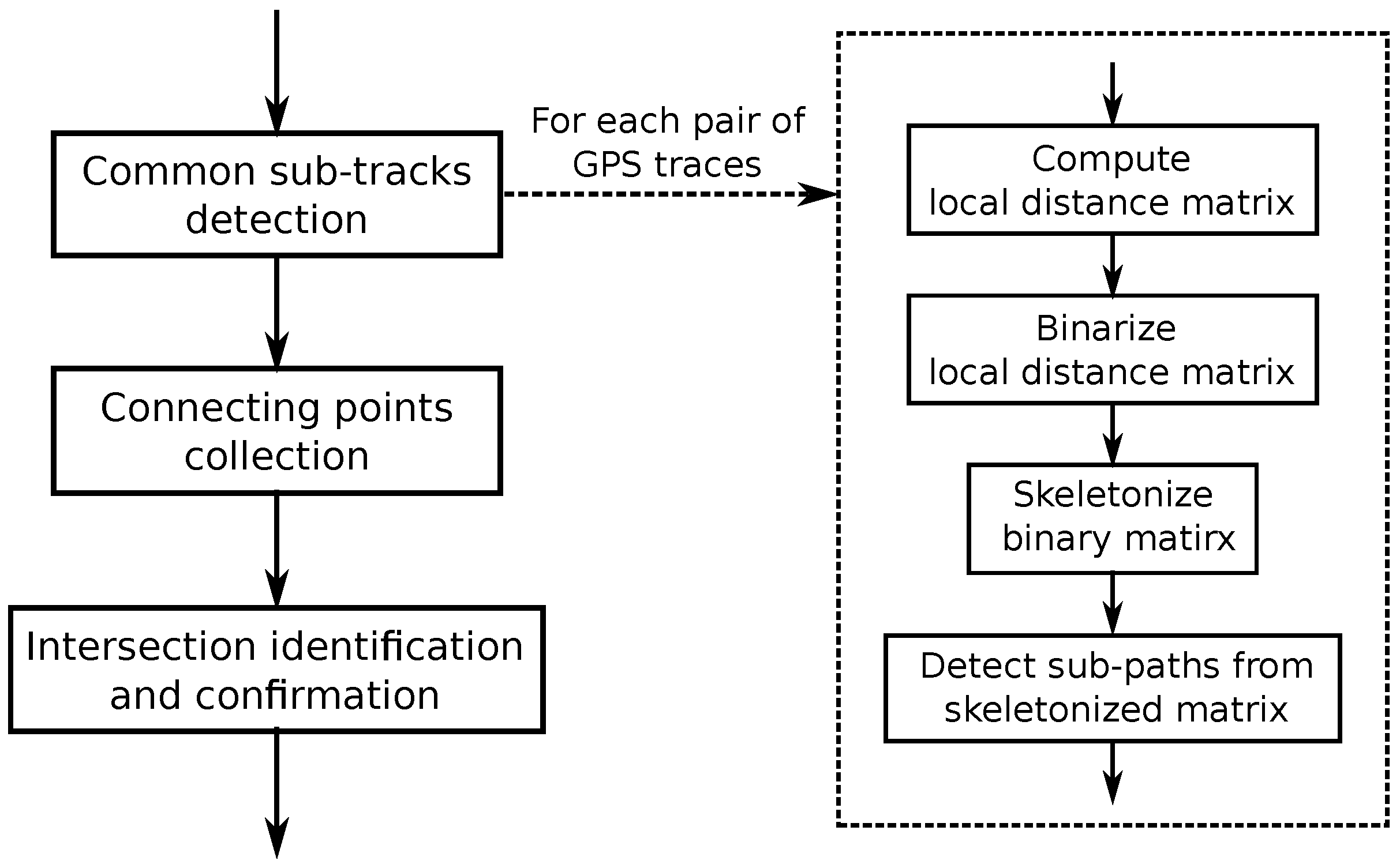
Figure 4.
Examples of binarized distance matrix. (a) example 2; (b) example 3.

Figure 5.
Examples of skeletonized distance matrix. (a) example 2; (b) example 3.
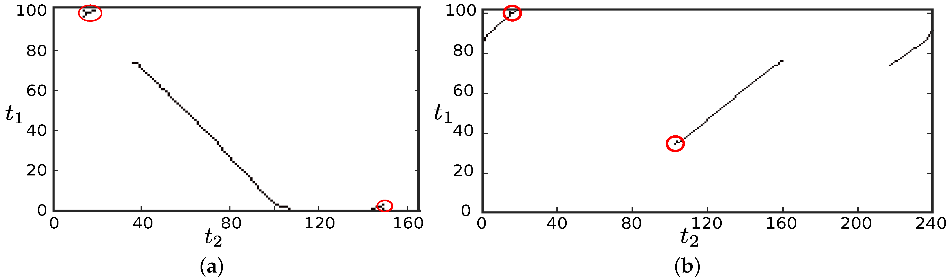
Figure 6.
Examples of “sub-paths”. (a) example 2; (b) example 3.
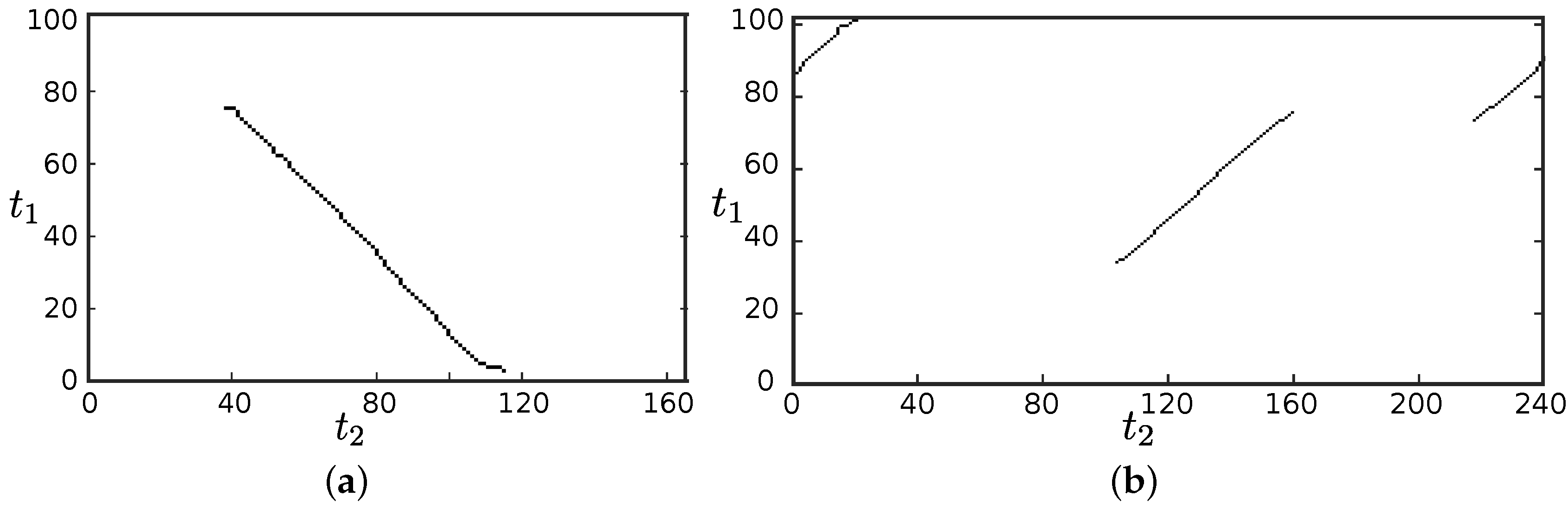
Figure 7.
A false positive intersection. One intersection candidate in the red circle is detected from the connecting points in green dots. It is a false positive because all of the connecting points are produced from 152 traces interconnecting with one single trace.
Figure 7.
A false positive intersection. One intersection candidate in the red circle is detected from the connecting points in green dots. It is a false positive because all of the connecting points are produced from 152 traces interconnecting with one single trace.
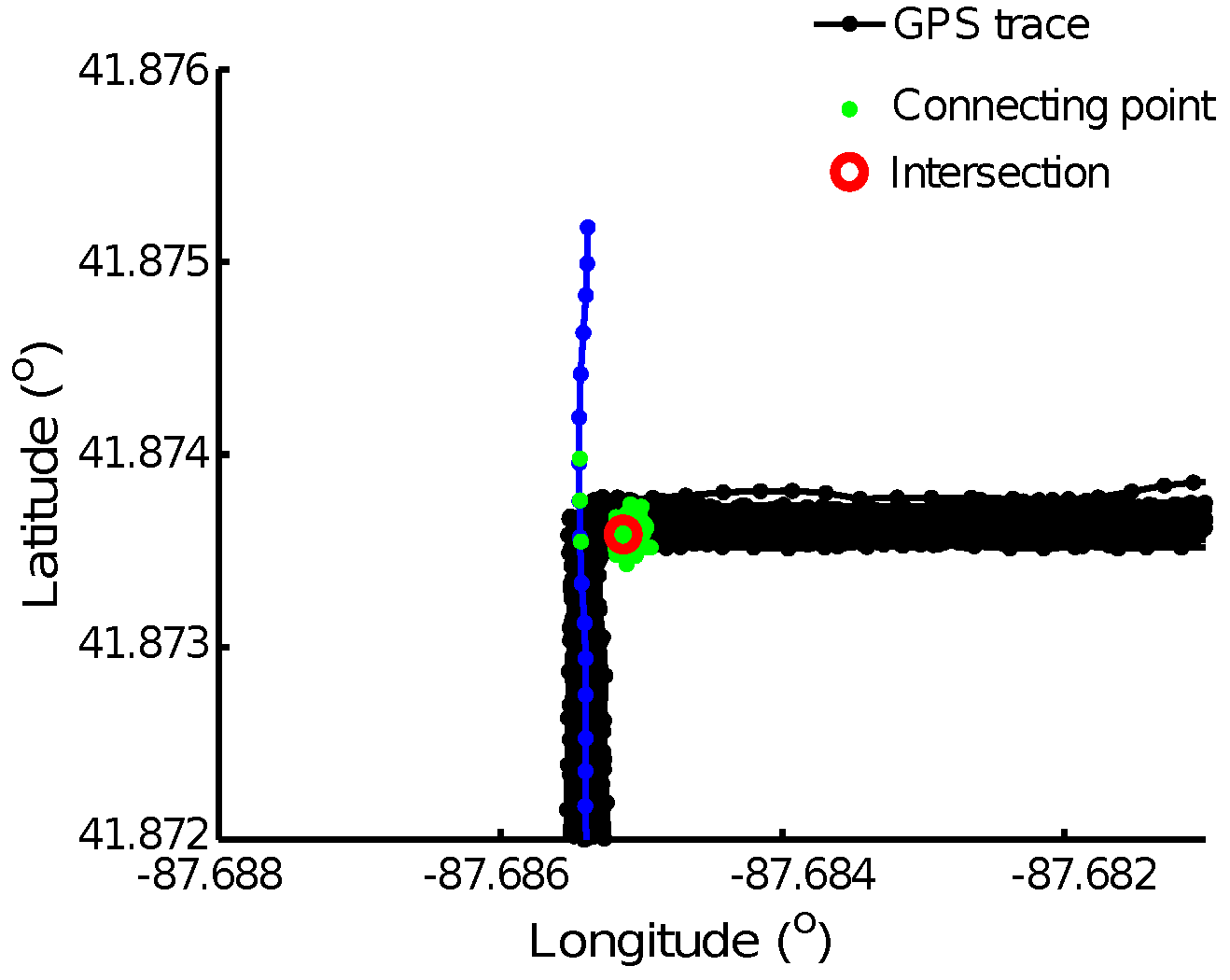
Figure 8.
GNSS traces and the ground truth intersections. A total of 889 GNSS traces are shown by the black lines with dots indicating the point locations, and the 33 ground truth intersections are depicted with blue circles.
Figure 8.
GNSS traces and the ground truth intersections. A total of 889 GNSS traces are shown by the black lines with dots indicating the point locations, and the 33 ground truth intersections are depicted with blue circles.

Figure 9.
Intersection candidates. The connecting points are depicted using green dots, and 37 intersection candidates using red circles.
Figure 9.
Intersection candidates. The connecting points are depicted using green dots, and 37 intersection candidates using red circles.

Figure 10.
Intersections. In total, 30 intersections are detected, including 29 true intersections shown with red circles and 1 spurious intersection with a red cross. Four ground truth intersections, indicated using blue circles, are detected unsuccessfully.
Figure 10.
Intersections. In total, 30 intersections are detected, including 29 true intersections shown with red circles and 1 spurious intersection with a red cross. Four ground truth intersections, indicated using blue circles, are detected unsuccessfully.

Figure 11.
Intersections detected using the turning points-based method.

Figure 12.
Intersections detected our previous LCSS method.
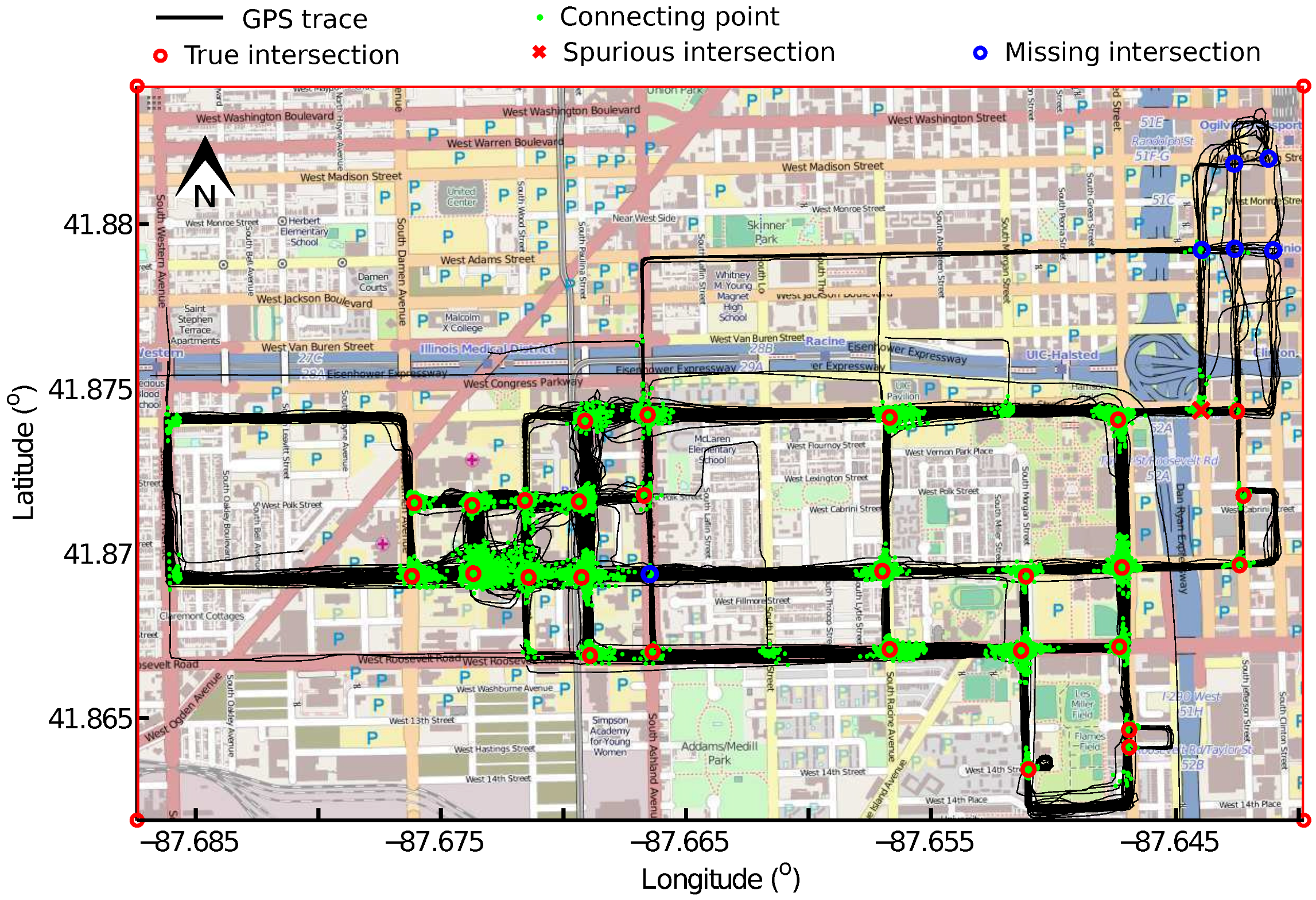
Figure 13.
Accuracy comparison.


Table 1.
Designations of the nine pixels in a window.
© 2017 by the authors. Licensee MDPI, Basel, Switzerland. This article is an open access article distributed under the terms and conditions of the Creative Commons Attribution (CC BY) license (http://creativecommons.org/licenses/by/4.0/).
Share and Cite
MDPI and ACS Style
Xie, X.; Philips, W. Road Intersection Detection through Finding Common Sub-Tracks between Pairwise GNSS Traces. ISPRS Int. J. Geo-Inf. 2017, 6, 311. https://doi.org/10.3390/ijgi6100311
AMA Style
Xie X, Philips W. Road Intersection Detection through Finding Common Sub-Tracks between Pairwise GNSS Traces. ISPRS International Journal of Geo-Information. 2017; 6(10):311. https://doi.org/10.3390/ijgi6100311
Chicago/Turabian StyleXie, Xingzhe, and Wilfried Philips. 2017. "Road Intersection Detection through Finding Common Sub-Tracks between Pairwise GNSS Traces" ISPRS International Journal of Geo-Information 6, no. 10: 311. https://doi.org/10.3390/ijgi6100311
Note that from the first issue of 2016, this journal uses article numbers instead of page numbers. See further details here.