Article

Spatio-Temporal Variability in a Turbid and Dynamic Tidal Estuarine Environment (Tasmania, Australia): An Assessment of MODIS Band 1 Reflectance

1
Institute for Marine and Antarctic Studies, University of Tasmania, Launceston 7250, Australia
2
Department of Environmental Health Sciences, Fairbanks School of Public Health, Indiana University-Purdue University, Indianapolis, IN 46202, USA
*
Author to whom correspondence should be addressed.
ISPRS Int. J. Geo-Inf. 2017, 6(11), 320; https://doi.org/10.3390/ijgi6110320
Submission received: 12 August 2017 / Revised: 9 October 2017 / Accepted: 16 October 2017 / Published: 25 October 2017

Abstract

:
Patterns of turbidity in estuarine environments are linked to hydrodynamic processes. However, the linkage between patterns and processes remains poorly resolved due to the scarcity of data needed to resolve fine scale highly dynamic processes in tidal estuaries. The application of remote sensing technology to monitor dynamic coastal areas such as estuaries offers important advantages in this regard, by providing synoptic maps of larger, constantly changing regions over consistent periods. In situ turbidity measurements were correlated against the Moderate Resolution Imaging Spectrometer Terra sensor 250 m surface reflectance product, in order to assess this product for examining the complex estuarine waters of the Tamar estuary (Australia). Satellite images were averaged to examine spatial, seasonal and annual patterns of turbidity. Relationships between in situ measurements of turbidity and reflectance is positively correlated and improves with increased tidal height, a decreased overpass-in situ gap, and one day after a rainfall event. Spatial and seasonal patterns that appear in seasonal and annual MODIS averages, highlighting the usefulness of satellite imagery for resource managers to manage sedimentation issues in a degraded estuary.

Graphical Abstract

1. Introduction

Monitoring hydrodynamic processes, agricultural practices, urban discharges, and the distribution, source and flux of suspended materials and pollutants in coastal and estuarine waters requires measurement of biological, hydromorphological and physio-chemical water quality parameters. An important parameter to measure is typically turbidity. Turbidity may affect the physical properties of the water column, such as temperature, dissolved oxygen content, sunlight penetration [1,2]. Turbidity can alter the physical structure of benthic habitat, which will affect benthic flora and fauna [3,4,5,6,7]. High turbidity can also damage water management infrastructure and increase the maintenance costs for these structures [1,8]. In the case of water sanitization, high turbidity prevents efficient and effective chlorination of water because high concentrations of suspended solids may interfere with chlorine facilitated bacteria removal [9,10]. Thus, the estimation of water transparency or cloudiness through indicators such as total suspended solids (TSS, in mg/L) or turbidity is of critical importance.
Anthropogenic alteration of the hydrodynamics in upper Tamar Estuary and Esk Rivers in Northern Tasmania, Australia (Figure 1) has prompted the need to alleviate the consequences of excessive silt and to restore ecosystem goods and services of the estuary such as, commercial activities, navigation and marine transportation, recreational and landscape values, flood control and biodiversity. Such restoration efforts have included the removal of excessive siltation through dredging and silt raking [11,12]. However, as a result of these raking procedures, silt can re-suspend and mobilize in the water column resulting in increased turbidity, thus exacerbating existing problems [13,14,15].
Conventional in situ sampling observations have played an important role in understanding estuarine processes and patterns of turbidity in the Tamar estuary. The Tamar Estuary and Esk Rivers (TEER) Ecosystem Health and Assessment Program (EHAP) has sampled the estuary on a monthly basis to generate a report card to assess the health of the estuary using a variety of water quality variables [16]. However, the cost and the limited temporal and spatial scale over which the data is collected has been a limitation. The dynamic nature of estuarine systems necessitates finer-scale monitoring, both temporally and spatially. Remote sensing can help overcome the weaknesses of in situ sampling by providing comprehensive spatial and consistent temporal coverage [17].
Complementing capabilities of in situ sampling and remote sensing offers great advantages for the study of estuarine processes. Combining in situ data from single-point time series with remotely sensed spatial data allows for a greater elucidation of changes in turbidity throughout various seasons and conditions. The combination of in situ data and remotely sensed data can provide information on the complexity of these processes that control turbidity patterns. This provides managers a more comprehensive understanding of the extent of turbidity and the potential impact of dredging and raking activities on ecosystem goods and services. However, dynamic hydrodynamic processes, leading to changes in optical properties, can confound satellite retrieval of turbidity measurements. For example, it has been demonstrated that changes in the scattering coefficient can be brought about by differences in sediment particle properties such as grain size and composition [18]. Mass settling fluxes of sediments in the near-bed portion of estuaries can vary by three or four orders of magnitude in meso- and macro-tidal estuaries throughout a single tidal cycle [19]. In addition, multiple processes (e.g., tides, rainfall events, river discharge, and sediment re-suspension by winds and waves, etc.) influence turbidity patterns within estuaries across multiple temporal and spatial scale and can make it difficult to develop relationships between satellite and in situ measurements [20,21,22].
This study aims to assess the relationship between in situ measurements of turbidity in the Tamar River and atmospherically-corrected reflectance in Band 1 (620–670 nm) from the MODIS Terra sensor (reflectance product MOD09GQ; Rrs) and how such relationships change as a function of tides, satellites crossing time and days after rainfall. The overall objective is to assess the applicability of this NASA product to describe the spatial and temporal (annual and seasonal) variability of turbidity patterns within the Tamar River estuary. Although diverse estuaries around the world have been analysed for turbidity using this product [23,24,25,26,27] none to our knowledge have faced conditions similar to those of the Tamar estuary. A highly altered system with an elevated sedimentation rate interacting with mesotidal conditions are challenges of this estuary to demonstrate the capabilities and effectiveness of this technology.

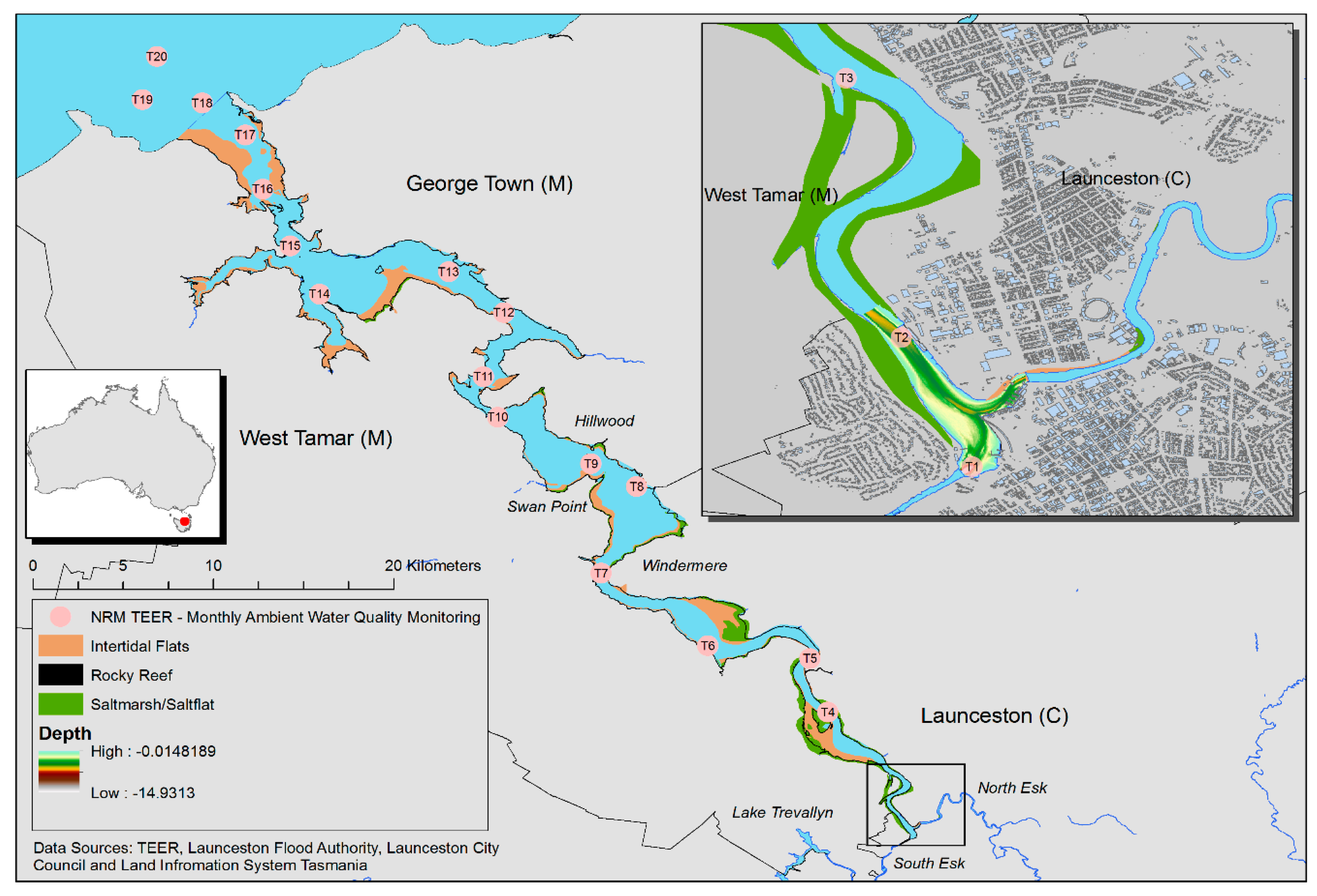
2. Study Area—Tamar River

The Tamar River is a tidal estuary located in Northern Tasmania, formed by the meeting between the North Esk and South Esk Rivers at Launceston and flows towards its mouth at Low Head before exiting into the Bass Strait (Figure 1). The river extends for about 65 km and in some locations is about 3 km wide. The area of the estuary is approximately 105 km2 and consists of a main channel (75 km2), intertidal mud flats (21 km2) and saltmarsh (7 km2) [28]. The Tamar has a high conservation significance, recording a large number of species not found elsewhere [29]. The subtidal substrates and habitats of the Tamar estuary are classified into six main groups—soft sediments, rocky reefs, giant kelp forests, algal beds, seagrass meadows and sponge gardens [30]. Aquaculture operations, including salmonid and abalone farming, are conducted in the Tamar estuary.
The entire Tamar River is tidal in nature, with a 3.5 m tide occurring twice daily [31]. Current velocities in the estuary can range from >12 m/s, when flow is mainly controlled by output from the North and South Esk rivers, to <1 m/s, which is the maximum diurnal tidal flow [32]. The tidal wave becomes increasingly asymmetric as it propagates upstream, providing a mechanism for the dominant tide-induced transport of sediments in the upstream direction. This upstream transport and anthropogenically reduced (dams and water diversion) flow from the North and South Esk Rivers [11,12] have contributed to sedimentation of the upper estuary. During floods, the combination of high river flow and tidal action flushes sediment into the lower reaches of the estuary [33]. However, reduced river flow and asymmetric tidal action pushes sediment back into the upper reaches [33] resulting in sedimentation rates varying from 3.3 to 33 mm/year depending on location [34]. Currently, silt “raking” is conducted during periods of high ebb flows resulting from spring tides and high winter run-off. Depending on flow rate, up to 240,000 m3 of silt has been moved further downstream [35] restoring the historical physical amenity to the upper estuary. Understanding the sediment dynamics of this system as well as the fate of the “raked” sediments has become crucially important [36].

3. Materials and Methods

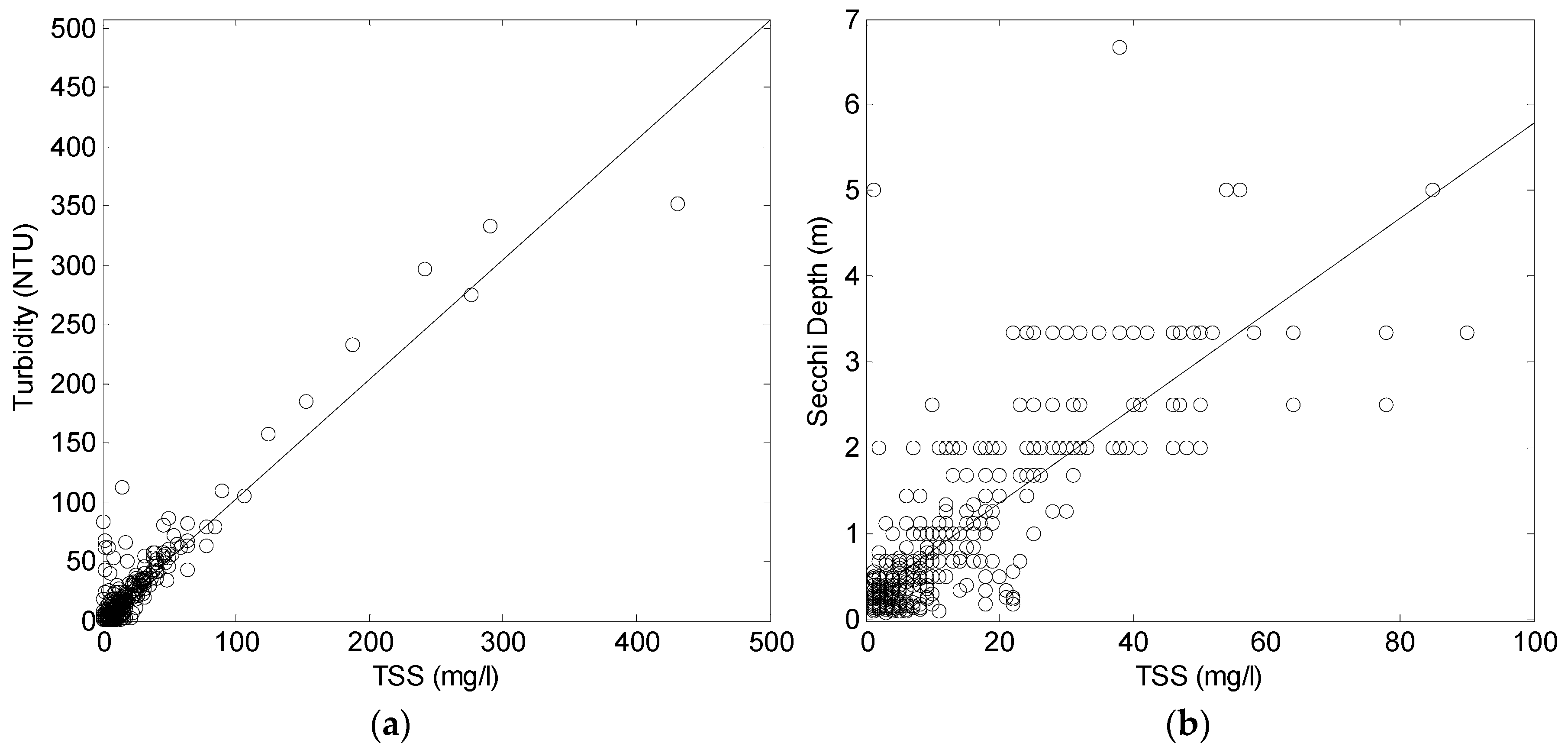
3.1. In Situ Measurements and Analysis

In situ measurements were obtained from the Tamar Estuary and Esk Rivers Ecosystem Health Assessment Program (TEER-EHAP). Measurements were taken monthly at 20 monitoring sites (n = 360) (Figure 2) between October 2009 to October 2011. The parameters used in this study include temperature, salinity, total suspended solids (TSS), turbidity and Secchi depth. These data were collected at the surface and at depth. For consistency, only surface measurements were considered. Meteorological data of daily rainfall and tidal heights were obtained from the Bureau of Meteorology [37].
In situ sampling procedures are outlined in the 2012 Tamar Estuary EHAP report [38] and are summarised here. At all sites, in situ water quality parameters (turbidity, temperature and salinity) were measured at discrete depths throughout the water column with a calibrated multi-probe water quality meter (Hydrolab DS5) lowered from the surface to the bottom of the water column. Water clarity and light penetration were measured by lowering a Secchi disk from the surface of the water and recording the distance where the disk is no longer visible. Surface and bottom water samples from each site were analysed using National Association of Testing Procedures (NATA)-accredited procedures for total suspended solids (TSS). The steps include direct collection into sample bottles, refrigeration at 1–4 °C for preservation, minimizing excessive turbulence to minimize presence of air bubbles in the water, and analysis of the sample within 24 h after collection. TSS samples were filtered (0.45 μm) in the lab to trap solids on the filter and measure the amount of sediments per volume of water. The different measures of turbidity, TSS and secchi disk were compared to ascertain consistency between methods of in situ measurements.

3.2. MODIS Data and Processing

The MODIS-terra satellite has been acquiring images of the earth since 2000 in 36 spectral bands at 250-m, 500-m and 1000-m spatial resolution. The red (Band 1, 620–670 nm) and NIR (Band 2, 841–876 nm) are available as a standard product, MOD09GQ, on a near daily basis at 250-m resolution and are sensitive for turbid water applications [39]. Doxaran et al. [24] has described the atmospheric correction process conducted for this product, which starts with the correction of MODIS L1B data for absorption and scattering effects, caused by gases and aerosols, and adjacency effects [2]. The resulting product is not corrected for skylight reflection at the air-water interface thus not very suitable for applications in “clear” waters such as the open ocean. However, it is still appropriate for estuarine waters due to their higher turbidity. It has been estimated, for estuarine waters, that about 80% of the reflectance in the red and between 70 to 90% of the reflectance in the near-infrared, are due to turbidity [2]. Therefore, the accuracy of atmospheric corrections is not as critical [2]. Blue and green bands were not tested due the coarse resolution (1 km) of these bands and the narrow width (maximum 3 km) of the estuary. In addition, these bands are not suitable for the Tamar estuary because of reduced reflectance at these wavelengths [24] in the presence of high concentrations of colored dissolved organic matter (CDOM) expected in a highly turbidity estuary [40,41].
Images (n = 1094) between 1 January 2009 to 31 December 2011 were downloaded from NASA’s Earth Observing System Data and Information System, Reverb ECHO [42]. Images were geographically referenced with the MODIS Reprojection Tool. A visual quality control was conducted to remove images which lacked data, were damaged by striping, or where clouds obscured the in situ sampling sites. Images with pixels outside the valid range, as specified MOD09GQ quality control descriptions [43], were removed from consideration. Reflectance readings for both the red and NIR bands were extracted from the remaining (n = 177) quality controlled images.

3.3. MODIS Reflectance Relationship to TSS, Turbidity and Secchi Depth

In order to determine the best relationship between reflectance values and turbidity, multiple linear regression analyses were conducted using reflectance of the red and NIR bands and their ratios. Relationships between reflectance readings and the in situ measurements were first analysed using all available matching pairs (between in situ and satellite overpass) from the same day regardless of tide, time difference or days after a rainfall event. Then, images were filtered to restrain matchup comparisons to only high and low tide. Successively, to evaluate the relevance and variability of these relationships as a function of time difference, datasets were organized into groups by time gap from the satellite overpass (10:30 a.m. local time). First, the few available matching pairs of the same hour (zero hours difference) were correlated, and then progressively increasing the sample size and time difference by adding one hour at a time up to ±7 h before and after the MODIS Terra overpass. Further, comparisons were made by considering tides and satellite crossing time simultaneously. After considering matchups before and after one-hour increments of satellite crossing time and then grouping the subsequent pairs into high tide and low tide, the matchup pairs were further restrained by days after rainfall. Matchups were grouped according to the number of days from the last rainfall event. For all cases, the coefficient of determination was recorded. Finally, annual and seasonal means of turbidity were created by averaging all valid imagery between 2009 and 2011. This was done to visually describe spatial, annual and seasonal, turbidity patterns in the estuary and to further compare turbidity measurements created by the correlation model against original in situ measurements.

4. Results

4.1. Water Mass Characteristics

In situ measurements of salinity, temperature, TSS, turbidity (NTU) and secchi depth, showed wide variation across the 20 sampling sites within the estuary, ranging from 0.01–35.5 psu, 5.7–24 °C, 1–431 mg/L, 0.1–351.5 NTU, and 0.10–16 m, respectively. As expected a robust linear relationship was obtained (Figure 2) between in situ measurements of TSS and turbidity (r2 = 0.89, n = 328, p < 0.001, y = x + 2.4) and in situ measurements of TSS below 100 mg/L and secchi depth (r2 = 0.65, n = 469, p < 0.001, y = 0.055x + 24). The relationship between TSS and secchi depth is less robust due to higher probability of sampling errors such as angular subtense, varying levels of sunlight, boat shading and observer bias. Due to the lack of in situ TSS measurements, hydrolab turbidity data was used for the remaining correlation analysis. Figure 2 confirms the reliability of turbidity measurements when compared with laboratory analysis of TSS samples.

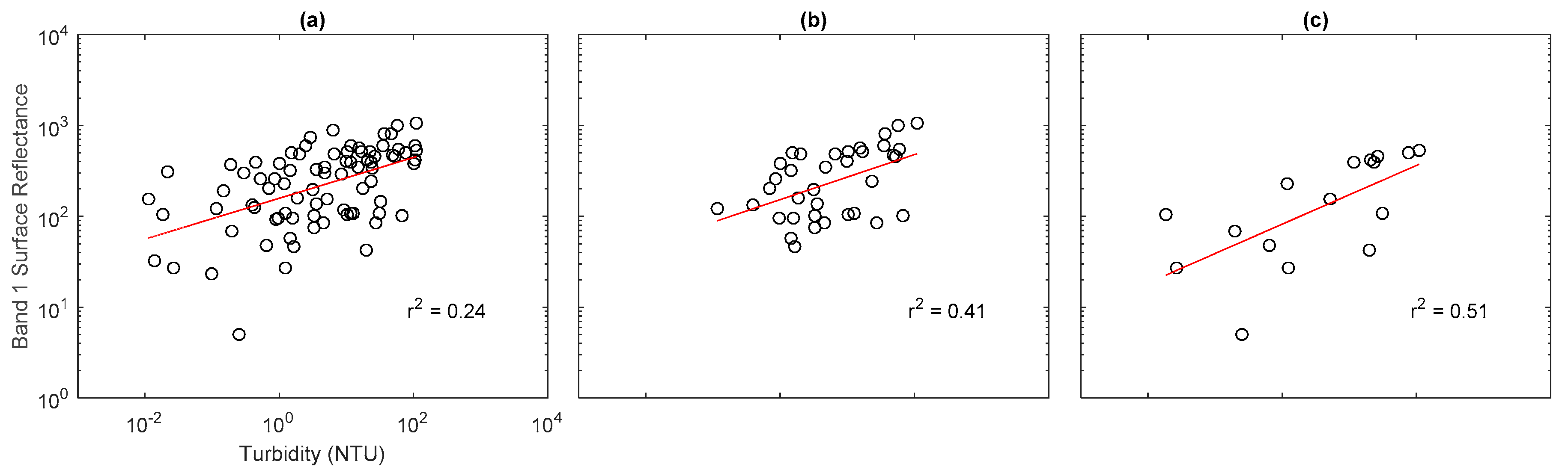
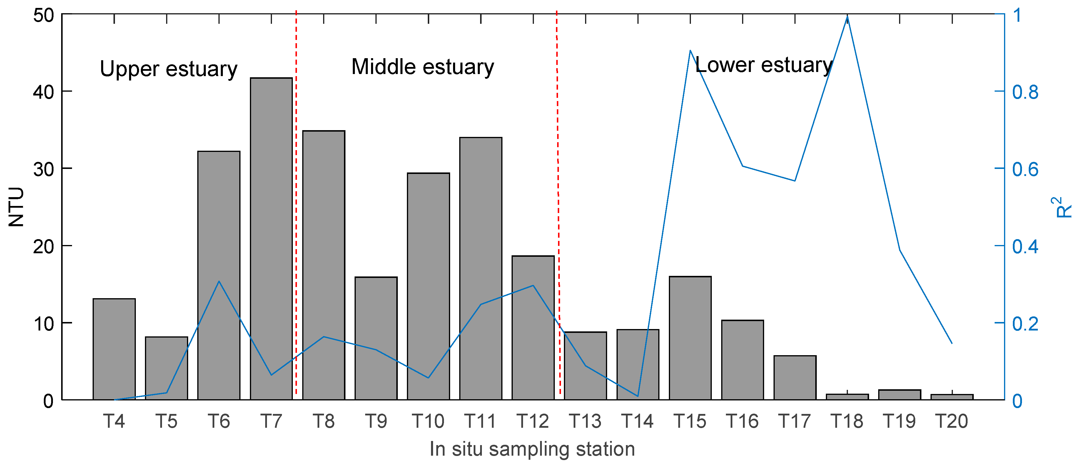
4.2. MODIS Reflectance vs. TSS and Turbidity

The analysis of the linear relationships between MODIS reflectance and in situ measurements of TSS, turbidity and Secchi depth are given in Table 1. The r values ranged from 0.005 to 0.3 with the Turbidity-Band 1 relationship (r2 = 0.2958) and Secchi depth-Band 1 (Red) relationship (r2 = 0.2819) being the highest. However, Secchi depth readings were not used for further analysis because their dependence on the amount of sunlight penetrating through the water column can be influenced by time and season of sampling, whereas turbidity is a fairly constant value. All relationships were low and those with red and NIR band ratios were not even significant (p > 0.1). This is contrary to what was found by [25] in the highly turbid although macrotidal estuary of the Gironde, France, where the reflectance ratio of MODIS bands 2 (NIR) and 1 (red) was best correlated with suspended particulate matter. In the present study, the three in situ parameters of water quality (TSS, turbidity and Secchi depth) were significantly correlated with the NIR band and the red bands. The red band was also best correlated with turbidity in the low-turbidity estuary of Tama Bay, FL, USA [2].

4.3. Correlation with Tides, Satellite crossing Time and Rainfall

The original coefficient of determination between all matching pairs of turbidity-Band 1 reflectance yielded 0.298 with 110 matching pairs (Table 1, Figure 3). The strength of the relationship did not improve when examining the reflectance as a power of turbidity (r2 = 0.287). After grouping all the matching pairs according to tidal heights (high or low), the r2 value improved from 0.298 to 0.478 at high tide (p < 0.01) with 50 matching pairs and 0.3181 at low tide (p < 0.01) with 60 matching pairs (Table 2). When considering satellite crossing time only (not shown in tables), the correlation improved from 0.298 to 0.445 (±2 h) (n = 66, p < 0.05). The highest correlation value was 0.997 at ±0 h. However, with a sample size of four (p = 0.06) this was not statistically significant at the 95% confidence level.
When considering tides and temporal gaps between in situ and satellite overpass, the best correlation occurred when in situ readings were taken within 2 h (±1 h) from satellite crossing time 0.5463 (n = 11; p < 0.01) at high tide and 0.3798 (n = 41; p < 0.01) at low tide (Table 2). Lastly, the strength of correlation increased from 0 days (0.4277; n = 42; p < 0.01) to 1 day (0.6066; n = 34; p < 0.01) after the last rainfall event. However, after 1 day, the correlation became weaker as the number of days after the last rainfall event increased, from r2 = 0.6066 to r2 = 0.009 at 7 days (Table 3, Figure 3).

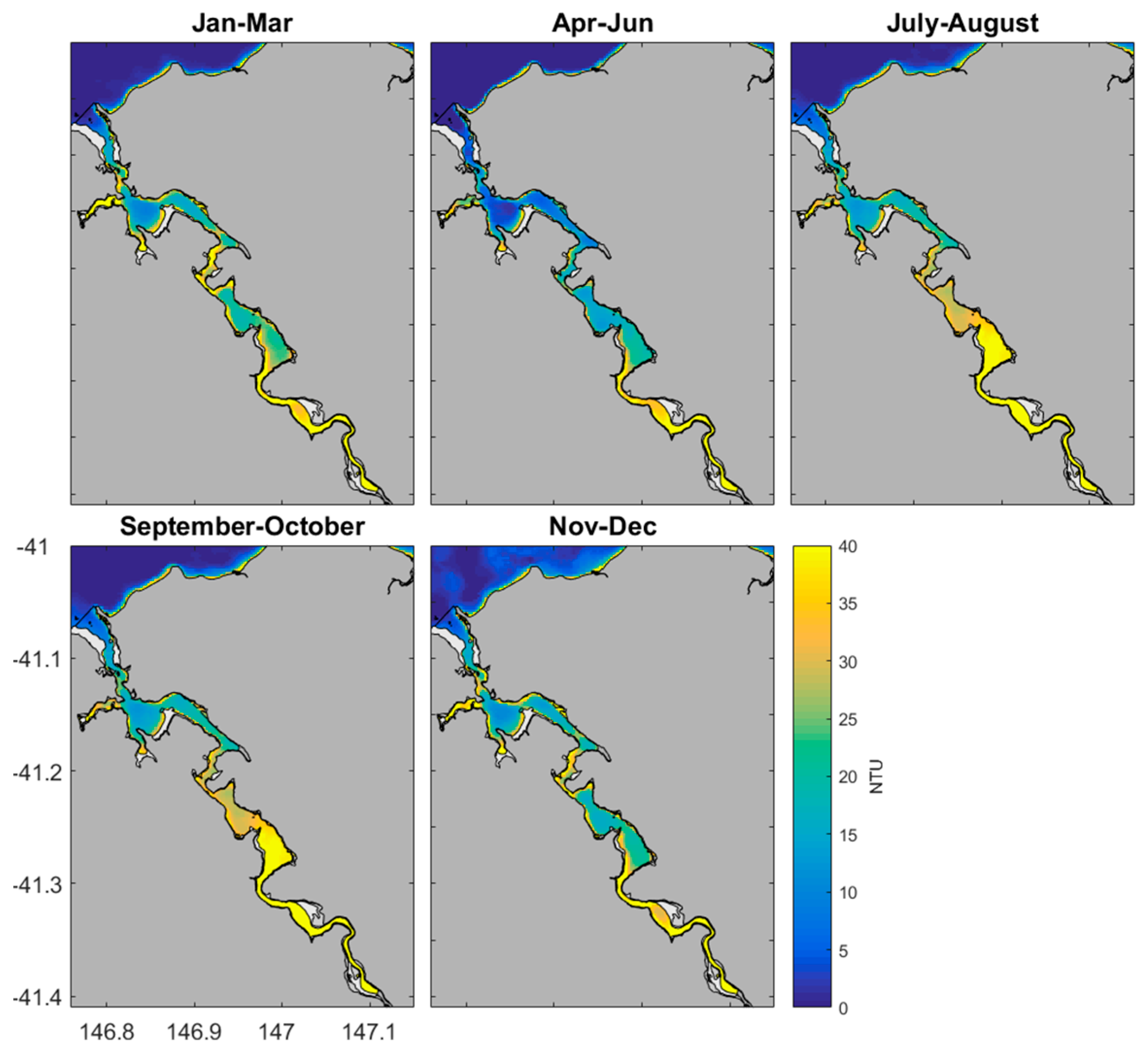
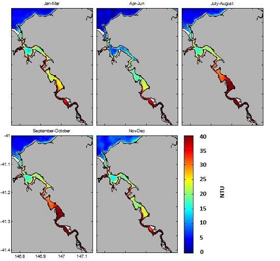
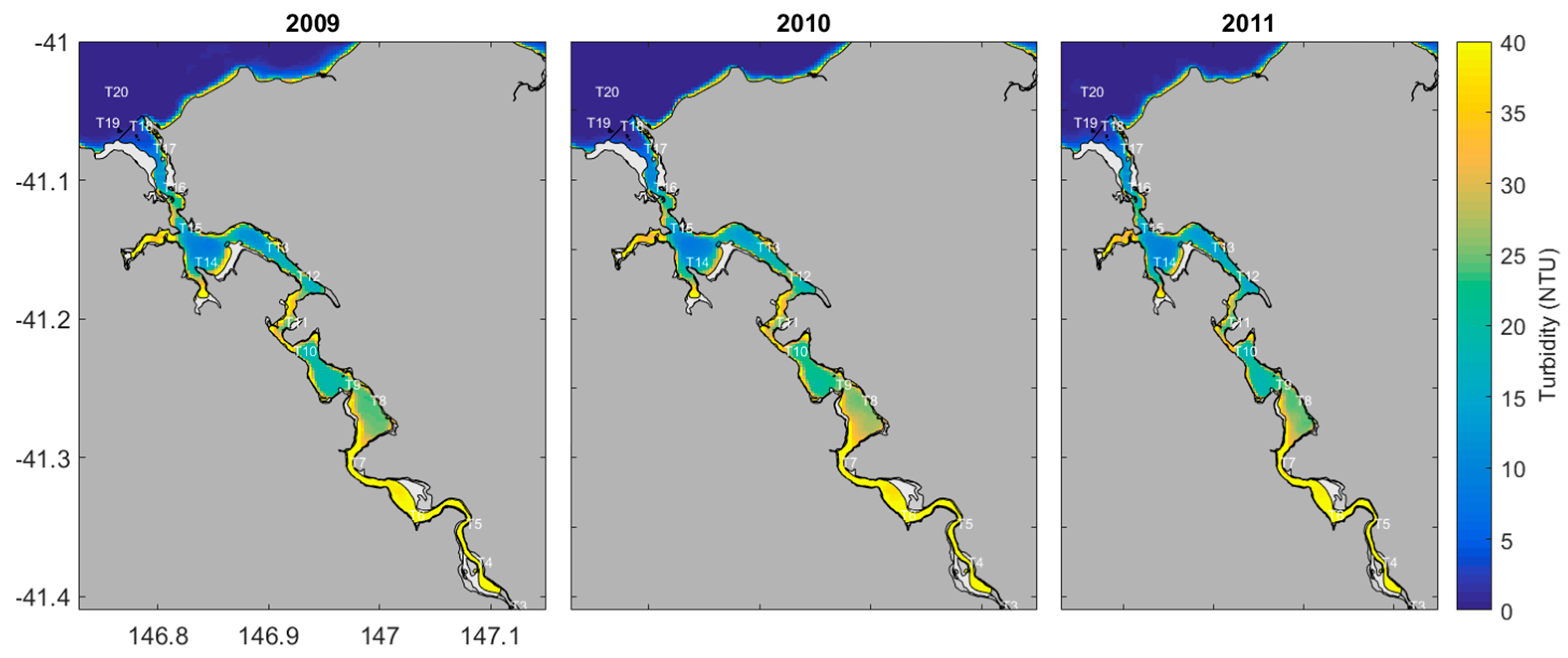
4.4. Satellite-Derived Climatology

Using a combination of images (n = 114) that had the highest correlation with in situ values at high tide (n = 49), ± 1 h after satellite overpass (n = 32) and one day after rainfall (n = 33), annual and seasonal composites of water surface reflectance were created. Reflectance values in the Figure 3a (n = 114) have been converted to turbidity values using the linear fit equation y = 0.1136x − 5.5956. Annual means of MOD09GQ Band 1 surface reflectance values, for the 2009–2011 period, delineate three distinct areas throughout the three years of imagery (Figure 4). These are, (1) the upper estuary, containing in situ sampling sites T1 to T7; (2) the middle estuary, covering primarily sites T8–T12; and (3) the lower estuary, containing sites T13–T20. Mean in situ turbidity values for each of the three distinct areas was approximately 32.7, 11.2, and 2.0 NTU for upper, middle and lower areas, respectively. Values within the respective areas ranged from 0.1–352, 0.1–332, 0.1–61.8 NTU.
Likewise, a distinct seasonal pattern is visible in the estuary. Higher levels of turbidity distribute across the upper half of the estuary between July to August and September to October encompassing zones T1–T12 (Figure 5). These months correspond to the austral winter with higher levels of rainfall. These months receive on average 70 mm of rainfall (based on a 80 years of data recorded by the Australian Bureau of Meteorology), compared to the drier parts of the year, November to June, which receives on average 50 mm of rainfall. Furthermore, the catchment area for the Tamar estuary comprises 15% of Tasmania’s land mass [16], suggesting that rainfall in other parts of the state may influence hydrodynamics and sediment loads in the estuary. A medium intensity in water turbidity is evident between November and March, with the lowest level of water turbidity between April and June. The middle estuary containing sites T8 to T12 appears to be the portion of the estuary that changes seasonally in terms of turbidity levels, with higher levels of turbidity appearing during the wetter months when river flow, due to the higher rainfall, increases. During the dryer months (November to March) and periods of low river flow and tidal asymmetry may be responsible for trapping fine sediments in the upper estuary.
The difference between model derived annual turbidity and the average in situ annual turbidity for each sampling station are shown in Figure 6. Differences in modelled and measured values ranged from 0.68 to 41.7 NTU. The greatest differences appear in the upper and middle estuary between stations T1–T12 (Figure 1). The correlations at these stations are generally lower than those at stations T13–T20. Both the differences between modelled and measured turbidity and the correlations between the values tend to improve in the less turbid waters of the lower estuary and estuary mouth, indicating that the more turbid and complex dynamics of the upper estuary confounds accurate retrieval of turbidity from MODIS Band 1 surface reflectance.

5. Discussion

Estuaries are dynamic systems and the fixed disconnection in place and time of in situ sampling inevitably loses spatio-temporal detail of this dynamic. In addition, this method is costly and is labour intensive. The Tamar River, Tasmania is an altered system with an elevated sedimentation rate and needs careful management. A more comprehensive and representative monitoring system is needed to fully understand the spatio-temporal dynamics of this system.
With better spatial and temporal coverage, remote sensing data can provide better monitoring coverage in a large areas like the Tamar Estuary. It has already been used in other geographical areas to monitor turbidity [2,23,25,26,27,44,45,46,47]. However, there is still a need to demonstrate the capabilities and effectiveness of this technology under meso- or macro-tidal regimes. This technology has never been demonstrated over the Tamar River, which is influenced by multiple processes, leading to a particularly high variability in the surface reflectance vs. turbidity relationship. Numerous factors affect the accurate retrieval of turbidity data from satellite, which explains the low determination coefficient obtained. Here we looked at several factors, which may influence retrieval of turbidity measurements from MODIS.
The relationship between surface reflectance and turbidity is influenced by sediment particle properties (size, composition) and the presence of organic particles (CDOM and chlorophyll). Such influence is expected to change drastically in an area with high variability (0.1–351.5 NTU) of turbidity such as the Tamar estuary. In other estuaries, extensive variability in turbidity has been reported to capture important differences between values of in situ and satellite-derived measurements even with 1 km spatial resolutions [48]. Processes that affect their distribution, such as localised upwelling, river discharge, tidal currents, frontal formation, waves, wind re-suspension, and biological growth vary over shorter spatial and temporal scales versus the relatively more homogeneous open ocean. All these factors combine to create an optically complex and dynamic system which presents challenges for the use of remotely sensed data. In addition, the highly reflective surface of land compared with that of water causes error flagging of remotely sensed water quality data at the coastline, limiting the analysis of narrow water bodies. This could help explain the low overall determination coefficient and the variation in correlation strength observed with tides and days after rainfall of the surface reflectance vs turbidity relationship.
The r2 value between turbidity and Band 1 surface reflectance increased from 0.2958 to 0.4784 and 0.3181 when categorized using high tide and low tide, respectively. The improvement in correlation suggests the need to consider tidal behavior when estimating turbidity with the MODIS MOD09GQ product. The Tamar Estuary is classified as a mesotidal (tidal range 2–4 m), drowned river valley [49], with tides ranging from 0.5 m to 3.5 m. The estuary also has a tidal regime transitional between semi-diurnal and diurnal with the characteristic tidal sequence being low low, low high, high low, and high high [50]. In some rare cases, strong tidal flows can generate unusual high turbidity by re-suspending the bottom sediments throughout the tidal cycle [51]. Tidal range, more than the tidal stage, influences the suspended sediment concentrations thus the turbidity. Changes between high and low tides cause changes in salinity and re-suspension processes that in turn lead to variations in particles properties and mineral composition [52,53]. This, in turn affects optical properties (absorption and backscattering) [54] and ultimately the surface reflectance vs turbidity relationships.
As expected, in general, the correlation improved with shorter time gap between in situ sampling and satellite overpass. The satellite overpass used in the analysis is 10:30 a.m. as this is the crossing time of the TERRA satellite. All in situ sampling was done within ±7 h from 10:30 a.m., with only 4 samplings taken at 10:30 a.m. Although these four samples provided the highest correlation (r2 = 0.9976, p = 0.06), presumably because of the temporal congruence between in situ and satellite data, this is not statistically significant at the 95% confidence level. In a highly dynamic estuary such as the Tamar, differences in biological and physical properties could be detected with in situ readings taken more than one hour before and after a satellite overpass. Although ideally, in situ readings should be taken at the same time as the satellite overpass, that would require sampling all 20 stations at the same time, not be feasible considering the limited resources of the TEER current monitoring program.
The coefficient of determination between turbidity and Band 1 surface reflectance taken the same day of a rainfall event was 0.4277 (n = 42; p < 0.01). The best coefficient of determination between both variables was detected the first day after a rainfall event (0.60; n = 34; p < 0.01) and then decreased in strength with the increasing time window. This change in the strength of the correlation may be related to the change in the nature of water turbidity in the estuary due to a variety of hydrodynamic processes, increased flow in the North and South Esk Rivers (Figure 1) and nonpoint source runoff. Storm water runoff, in the estuary and from the rivers, brings freshwater terrigenous sediments and organic material from the watershed [40,41]. These inputs change the salinity, particle properties, and mineral composition of sediments in the water column [54]. Such change affects the refractive index [55] and consequently the optical properties of the suspended particles [54], therefore influencing the strength of the relationship between turbidity and Band 1 surface reflectance. Errors in the surface reflectance retrievals are caused by, among other factors, thin clouds, water vapour and aerosols such as smog and dust. Those factors change during the days following a rainfall event, and have been suggested to be contributing factors to the improvement in the turbidity-Band 1 relationship, in a study conducted in Tampa Bay, Florida [2]. The presence of these atmospheric conditions are not sufficiently accounted for in the standard atmospheric correction algorithms and may introduce errors and inconsistencies during day zero of rainfall. This may help explain the improvement, in our study, from day zero (r2 = 0.4277) to day one (r2 = 0.6066) after rainfall.
A relatively small portion of the watershed in the Tamar Estuary is covered by adjacent urbanised areas and a large portion of it is covered by agriculture land use, a practice widely known for the introduction of sediments into waterways [16]. Under such circumstances, rainfall may lead to a rapid increase in turbidity. Indeed, in the study conducted in the estuary of Tampa Bay, FL, USA, the authors suggested that the impervious surfaces and prevalence of storm water retention ponds of this highly urbanized watershed prevents rapid transport of sediments from adjacent sources to the bay shortly after rainfall. However, a lag time for sediments from rural lands at the head waters would eventually increase turbidity with more days after rainfall [2]. A similar process has been reported for Mobile Bay, AL, USA [56]. Complementarily, another study conducted in Tampa Bay timidly suggest an inverse relationship between the temporal trend lines of water turbidity and urban land use change in the watershed [57]. These characteristics may explain why in Tampa Bay, a bay with most of its shoreline surrounded by urban land use, the weakest correlation between turbidity and Band 1 surface reflectance has been detected right after rainfall events, a period during which sediment-free water is discharged from the adjacent urban watershed. Then, a progressive improvement in the correlation occurs with days after rainfall, as the lag time allows for sediments from more rural upstream waters to reach the bay [2]. Unlike Tampa Bay, the Tamar River watershed has a greater proportion of rural and agriculture land cover than urban and its waters are more turbid. Under conditions of higher water turbidity, further increasing water turbidity with more days after rainfall (due to the lag time between rainfall and sediments entering the estuary) may be responsible for the decrease in the turbidity-Band 1 relationship (Table 3), especially considering a higher content of organic matter being brought with the runoff from a mostly rural watershed. In agreement, the estimation of turbidity using the model based on the turbidity vs. reflectance relationship tends to be more accurate (less difference from the average in situ turbidity) toward sites downstream (Figure 6), which may suggest better performance of the model in less turbid waters.
Precipitation, land cover/land use, flow rate and runoff source are all determinant factors explaining the behavior of water turbidity and its correlation with band 1 reflectance. The combined effect from the different factors in the Tamar estuary is currently unknown. Therefore, more research is required to understand the turbidity patterns in this estuary, primarily, on the influence of tidal re-suspension to sediments.
Several challenges lie in the path of measuring and understanding these complex relationships, particularly around the operational aspects of using remote sensing in the environmental management context [58]. Several suggestion have been made in this respect and include, providing unrestricted access to monitoring equipment when weather and tidal conditions open rare windows of opportunity [59], the further development of cost effective and innovative platforms, such as UAVs (unmannered aerial vehicles), and promoting funding for multidisciplinary research campaigns. Such research campaigns should incorporate a combination of remote and in situ sampling techniques, as has been demonstrated in algal blooms studies [59] and estuarine plume dynamics [60]. This approach may assist in overcoming some of the traditional problems associated with remote sensing, such as measurements limited to the top few feet of the water column and cloud cover obstruction [61].

6. Conclusions

Multiple regression analyses were conducted to explore the relationship between in situ measurements of turbidity in the Tamar River and atmospherically-corrected reflectance on the red and NIR bands and their ratios from the MODIS Terra sensor reflectance MOD09GQ product. The relationship between turbidity and Band 1 (620–670 nm) reflectance was found to be the best of the four options. The strength of this positive relationship improved when considering tidal elevation, a decreased gap between satellite overpass and in situ sampling and fewer days after the last rainfall event. The highest correlation occurs when the matched data between in situ turbidity and Band 1 reflectance was retrieved 1 day after the last rainfall event. The turbidity-Band 1 relationship (r2) tends to improve in sites located downstream, suggesting better performance of the model (and the product MOD09GQ, Band 1) in less turbidity waters.
Annual means of surface water reflectance from this standard NASA product, for the 2009–2011 period, clearly detect turbidity to be higher in the upper estuary and lower in the lower estuary where there is more tide influence. Likewise, this product detected the highest water turbidity during the seasonal period between July and October. A medium intensity in water turbidity was detected between November and March. Lastly, the lowest level of water turbidity was detected between April and June. Overall, this study demonstrated the feasibility of using the MOD09GQ Band 1 in the Tamar Estuary to appreciate the seasonal or annual trend in sediment movement.

Acknowledgments

Thank you to the TEER EHAP program for providing the in situ data. We would like to thank the four anonymous reviewers for their thoughtful comments.

Author Contributions

Andrew M. Fischer and Max J. Moreno-Madriñán conceived and designed the research and analyzed the data and results. Max J. Moreno-Madriñán provided the instruction for downloading and processing of satellite imagery. Daniel Pang downloaded the satellite imagery, processed the data and performed the statistical analysis. Andrew M. Fischer, Daniel Pang, Ian Kidd, and Max J. Moreno-Madriñán wrote the manuscript.

Conflicts of Interest

The authors declare no conflict of interest.

References

  1. Warren, J.A.; Berner, J.E.; Curtis, T. Climate change and human health: Infrastructure impacts to small remote communities in the north. Int. J. Circumpolar Health 2005, 64, 487–497. [Google Scholar] [CrossRef] [PubMed]
  2. Moreno-Madrinan, M.J.; Al-Hamdan, M.Z.; Rickman, D.L.; Muller-Karger, F.E. Using the Surface Reflectance MODIS Terra Product to Estimate Turbidity in Tampa Bay, Florida. Remote Sens. 2010, 2, 2713–2728. [Google Scholar] [CrossRef]
  3. Pratt, D.R.; Pilditch, C.A.; Lohrer, A.M.; Thrush, S.F. The effects of short-term increases in turbidity on sandflat microphytobenthic productivity and nutrient fluxes. J. Sea Res. 2014, 92, 170–177. [Google Scholar] [CrossRef]
  4. Johansen, J.L.; Jones, G.P. Sediment-induced turbidity impairs foraging performance and prey choice of planktivorous coral reef fishes. Ecol. Appl. 2013, 23, 1504–1517. [Google Scholar] [CrossRef] [PubMed]
  5. Hasenbein, M.; Komoroske, L.M.; Connon, R.E.; Geist, J.; Fangue, N.A. Turbidity and salinity affect feeding performance and physiological stress in the endangered delta smelt. Integr. Comp. Biol. 2013, 53, 620–634. [Google Scholar] [CrossRef] [PubMed]
  6. Xu, H.; Wolanski, E.; Chen, Z. Suspended particulate matter affects the nutrient budget of turbid estuaries: Modification of the LOICZ model and application to the Yangtze Estuary. Estuar. Coast. Shelf Sci. 2013, 127, 59–62. [Google Scholar] [CrossRef]
  7. Matveev, V.F.; Steven, A.D.L. The effects of salinity, turbidity and flow on fish biomass estimated acoustically in two tidal rivers. Mar. Freshw. Res. 2013. [Google Scholar] [CrossRef]
  8. Tal, A. Seeking sustainability: Israel’s evolving water management strategy. Science 2006, 313, 1081–1084. [Google Scholar] [CrossRef] [PubMed]
  9. Tegtmeier, E.M.; Duffy, M.D. External costs of agricultural production in the United States. Int. J. Agric. Sustain. 2004, 2, 1–20. [Google Scholar] [CrossRef]
  10. Juntunen, P.; Liukkonen, M.; Lehtola, M.J.; Hiltunen, Y. Dynamic soft sensors for detecting factors affecting turbidity in drinking water. J. Hydroinform. 2013, 15, 416–426. [Google Scholar] [CrossRef]
  11. Davis, J.; Kidd, I.M. Identifying Major Stressors: The Essential Precursor to Restoring Cultural Ecosystem Services in a Degraded Estuary. Estuar. Coast. 2012, 35, 1007–1017. [Google Scholar] [CrossRef]
  12. Kidd, I.M.; Chai, S.; Fischer, A. Tidal Heights in Hyper-Synchronous Estuaries. Nat. Resour. 2014, 5, 607–615. [Google Scholar] [CrossRef]
  13. Newcombe, C.P.; MacDonald, D.D. Effects of suspended sediments on aquatic ecosystems. N. Am. J. Fish. Manag. 1991, 11, 72–82. [Google Scholar] [CrossRef]
  14. Chutter, F.M. The effects of silt and sand on the invertebrate fauna of streams and rivers. Hydrobiologia 1969, 34, 57–76. [Google Scholar] [CrossRef]
  15. Wilber, D.H.; Clarke, D.G. Biological effects of suspended sediments: A review of suspended sediment impacts on fish and shellfish with relation to dredging activities in estuaries. N. Am. J. Fish. Manag. 2001, 21, 855–875. [Google Scholar] [CrossRef]
  16. Tamar Estuary and Esk Rivers (TEER) Program. Tamar Estuary 2016 Report Card, Ecosystem Health Assessment Program: Monitoring Period December 2014–November 2015; NRM North: Launceston, Australia, 2017. [Google Scholar]
  17. Miller, R.L.; Liu, C.C.; Buonassissi, C.J.; Wu, A.M. A multi-sensor approach to examining the distribution of total suspended matter (TSM) in the Albemarle-Pamlico estuarine system, NC, USA. Remote Sens. 2011, 3, 962–974. [Google Scholar] [CrossRef]
  18. Binding, C.E.; Bowers, D.G.; Mitchelson-Jacob, E.G. Estimating suspended sediment concentrations from ocean colour measurements in moderately turbid waters; the impact of variable particle scattering properties. Remote sens. Environ. 2005, 94, 373–383. [Google Scholar] [CrossRef]
  19. Manning, A.J.; Bass, S.J. Variability in cohesive sediment settling fluxes: Observations under different estuarine tidal conditions. Mar. Geol. 2006, 235, 177–192. [Google Scholar] [CrossRef]
  20. Freitas, P.T.; Asp, N.E.; e Souza-Filho, P.W.M.; Nittrouer, C.A.; Ogston, A.S.; da Silva, M.S. Tidal influence on the hydrodynamics and sediment entrapment in a major Amazon River tributary–Lower Tapajós River. J. S. Am. Earth Sci. 2017, 79, 189–201. [Google Scholar] [CrossRef]
  21. Joshi, I.D.; D’Sa, E.J.; Osburn, C.L.; Bianchi, T.S. Turbidity in Apalachicola Bay, Florida from Landsat 5 TM and Field Data: Seasonal Patterns and Response to Extreme Events. Remote Sens. 2017, 9, 367. [Google Scholar] [CrossRef]
  22. Constantin, S.; Constantinescu, Ș.; Doxaran, D. Long-term analysis of turbidity patterns in Danube Delta coastal area based on MODIS satellite data. J. Mar. Syst. 2017, 170, 10–21. [Google Scholar] [CrossRef]
  23. Amin, A.R.M.; Abdullah, K.; Lim, H.S.; Embong, M.F.; Ahmad, F.; Yaacob, R. Development of Regional TSS Algorithm over Penang using Modis Terra (250 M) Surface Reflectance Product. Ekológia (Bratislava) 2016, 35, 289–294. [Google Scholar] [CrossRef]
  24. Chen, Z.; Hu, C.; Muller-Karger, F. Monitoring turbidity in Tampa Bay using MODIS/Aqua 250-m imagery. Remote Sens. Environ. 2007, 109, 207–220. [Google Scholar] [CrossRef]
  25. Doxaran, D.; Froidefond, J.M.; Castaing, P.; Babin, M. Dynamics of the turbidity maximum zone in a macrotidal estuary (the Gironde, France): Observations from field and MODIS satellite data. Estuar. Coast. Shelf Sci. 2009, 81, 321–332. [Google Scholar] [CrossRef]
  26. Moreno-Madriñán, M.J.; Rickman, D.L.; Ogashawara, I.; Irwin, D.E.; Ye, J.; Al-Hamdan, M.Z. Using remote sensing to monitor the influence of river discharge on watershed outlets and adjacent coral reefs: Magdalena River and Rosario Islands, Colombia. Int. J. Appl. Earth Obs. Geoinform. 2015, 38, 204–215. [Google Scholar] [CrossRef]
  27. Kumar, A.; Equeenuddin, S.M.; Mishra, D.R.; Acharya, B.C. Remote monitoring of sediment dynamics in a coastal lagoon: Long-term spatio-temporal variability of suspended sediment in Chilika. Estuar. Coast. Shelf Sci. 2016, 170, 155–172. [Google Scholar] [CrossRef]
  28. Sharples, C. Indicative Mapping of Tasmanian Coastal Vulnerability to Climate Change and Sea-Level Rise: Explanatory Report, 2nd ed.; Consultant Report to Department of Primary Industries and Water, Tasmania; Department of Primary Industries & Water Tasmania: Hobart, Australia, 2006.
  29. Ellison, J.C.; Sheehan, M.R. Past, Present and Futures of the Tamar Estuary, Tasmania. In Estuaries of Australia in 2050 and Beyond; Springer: Dordrecht, The Netherlands, 2014; pp. 69–89. [Google Scholar]
  30. Maynard, D.; Gaston, T. Beneath the Tamar: More that Silt; NRM North: Launceston, Australia, 2010. [Google Scholar]
  31. Smith, B.J. Tamar Estuary. In The Companion to Tasmanian History; Centre for Tasmanian Historical Studies, University of Tasmania: Hobart, Australia, 2006; Available online: http://www.utas.edu.au/library/companion_to_tasmanian_history/T/Tamar%20estuary.htm (accessed on 31 March 2013).
  32. Wood, W.F. Report on the Tamar Estuary Physical Study; Study number 2; Department of Environmental and Land Management, Northern Regional Office: Launceston, Australia, 1992. [Google Scholar]
  33. Gunawardana, D.; Locatelli, A. Tamar Estuary Management Plan; Northern Tasmanian Natural Resource Management Association Inc: Launceston, Australia, 2008. [Google Scholar]
  34. Armstrong, N.S. Holocene Sedimentation and Heavy-Metal Contamination in the Industrialised Tamar River Estuary. Honours Thesis, University of Wollongong, Wollongong, Australia, 2005. [Google Scholar]
  35. Kidd, I.M.; Davis, J.; Seward, M.; Fischer, A. Bathymetric rejuvenation strategies for a degraded estuary. Ocean Coast. Manag. 2017, 142, 98–110. [Google Scholar] [CrossRef]
  36. ETS Worldwide Ltd. Tracer Analysis of Sediment Redistribution of Tamar Estuary for Launceston Flood Authority; Australian Maritime College Search: Launceston, Australia, 2015. [Google Scholar]
  37. Australian Government Bureau of Meteorology. Available online: http://www.bom.gov.au (accessed on 7 June 2013).
  38. Tamar Estuary and Esk Rivers Ecosystem Health Assessment Program (TEER EHAP). Tamar Estuary Ecosystem Health Assessment Program Monitoring Report 2012; NRM North: Launceston, Australia, 2012.
  39. Hu, C.; Chen, Z.; Clayton, T.D.; Swarzenski, P.; Brock, J.C.; Muller-Karger, F.E. Assessment of estuarine water-quality indicators using MODIS medium-resolution bands. Remote Sens. Environ. 2004, 93, 423–441. [Google Scholar] [CrossRef]
  40. Moran, M.A. Distribution of terrestrially derived dissolved organic matter on the southeastern U.S. continental shelf. Limnol. Oceanogr. 1991, 36, 1134–1149. [Google Scholar] [CrossRef]
  41. Moran, M.A.; Hodson, R.H. Dissolved humic substances of vascular plant origin in a coastal marine environment. Limnol. Oceanogr. 1994, 39, 762–771. [Google Scholar] [CrossRef]
  42. Reverb ECHO, EOSDIS NASA’s Earth Observing Systems, Data Administration System. Available online: https://reverb.echo.nasa.gov/ (accessed on 10 February 2013).
  43. Land Processes Distributed Active Archive Center. Available online: https://lpdaac.usgs.gov/tools/modis_reprojection_tool (accessed on 12 March 2013).
  44. Petus, C.; Chust, G.; Gohin, F.; Doxaran, D.; Froidefond, J.M.; Sagarminaga, Y. Estimating turbidity and total suspended matter in the Adour River plume (South Bay of Biscay) using MODIS 250-m imagery. Cont. Shelf Res. 2010, 30, 379–392. [Google Scholar] [CrossRef]
  45. Wang, M.; Shi, W.; Tang, J. Water property monitoring and assessment for China’s inland Lake Taihu from MODIS-Aqua measurements. Remote Sens. Environ. 2011, 115, 841–854. [Google Scholar] [CrossRef]
  46. Wu, G.; Leeus, J.; Skidmore, A.K.; Prins, H.H.; Liu, Y. Concurrent monitoring of vessels and water turbidity enhances the strength of evidence in remotely sensed dredging impact assessment. Water Res. 2007, 41, 3271–3280. [Google Scholar] [CrossRef] [PubMed]
  47. Wu, M.; Zhang, W.; Wang, X.; Luo, D. Application of MODIS satellite data in monitoring water quality parameters of Chaohu Lake in China. Environ. Monit. Assess. 2009, 148, 255–264. [Google Scholar] [CrossRef] [PubMed]
  48. Ody, A.; Doxaran, D.; Vanhellemont, Q.; Nechad, B.; Novoa, S.; Many, G.; Bourrin, F.; Verney, R.; Pairaud, I.; Gentili, B. Potential of high spatial and temporal ocean color satellite data to study the dynamics of suspended particles in a micro-tidal river plume. Remote Sens. 2016, 8, 245. [Google Scholar] [CrossRef] [Green Version]
  49. Edgar, G.J.; Barrett, N.S.; Graddon, D.J.; Last, P.R. The conservation significance of estuaries: A classification of Tasmanian estuaries using ecological, physical and demographic attributes as a case study. Biol. Conserv. 2000, 92, 383–397. [Google Scholar] [CrossRef]
  50. Kleypas, J.A. Coral Reef Development under Naturally Turbid Conditions: Fringing Reefs near Broad Sound, Australia. Coral Reefs 1996, 15, 153–167. [Google Scholar] [CrossRef]
  51. Fennessy, M.J.; Dyer, K.R.; Huntley, D.A. Size and settling velocity distributions of flocs in the Tamar estuary during a tidal cycle. Neth. J. Aquat. Ecol. 1994, 28, 275–282. [Google Scholar] [CrossRef]
  52. Eisma, D.; Li, A. Changes in suspended-matter floc size during the tidal cycle in the Dollar Estuary. Neth. J. Sea Res. 1993, 31, 107–117. [Google Scholar] [CrossRef]
  53. Doxaran, D.; Froidefond, J.-M.; Castaing, P. Remote-sensing reflectance of turbid sediment-dominated water. Reduction of sediment type variations and changing illumination conditions effects by use of reflectance ratios. Appl. Opt. 2003, 42, 2623–2634. [Google Scholar] [CrossRef] [PubMed]
  54. Lahet, F.; Ouillon, S.; Forget, P. A Three-component model of ocean color and its application in the Ebro River mouth area. Remote Sens. Environ. 2000, 72, 181–190. [Google Scholar] [CrossRef]
  55. Goransson, G.; Larson, M.; Bendz, D. Variation in turbidity with precipitation and flow in a regulated river system—river Gota Alv, SW Sweden. Hydrol. Earth Syst. Sci. 2013, 17, 2529–2542. [Google Scholar] [CrossRef]
  56. Estes, M.G.; Al-Hamdan, M.; Thom, R.; Quattrochi, D.; Woodruff, D.; Judd, C.; Jean, E.; Watson, B.; Rodriguez, H.; Johnson, H. Watershed and hydrodynamic modeling for evaluating the impact of land use change on submerged aquatic vegetation and seagrasses in Mobile Bay. In Proceedings of the Oceans 2009 MTS/IEEE Conference, Biloxi, MS, USA, 26–29 October 2009. [Google Scholar]
  57. Moreno-Madriñán, M.J.; Al-Hamdan, M.Z.; Rickman, D.L.; Ye, J. Relationship Between Watershed Land-Cover/Land-Use Change and Water Turbidity Status of Tampa Bay Major Tributaries, Florida, USA. Water Air Soil Pollut. 2012, 223, 2093–2109. [Google Scholar] [CrossRef]
  58. Elsner, P.; Spencer, T.; Moeller, I.; Smith, G.M. Multitemporal Remote Sensing of Coastal Sediment Dynamics. In Environmental Remote Sensing and Systems Analysis; CRC Press: Boca Raton, FL, USA, 2012. [Google Scholar]
  59. Ryan, J.P.; Dierrsen, H.M.; Kudela, R.M.; Scholin, C.A.; Johnson, K.S.; Sullivan, J.M.; Fischer, A.M.; Enaney, P.R.; Chavez, F.P. Coastal ocean physics and red tides. Oceanography 2005, 18, 247–255. [Google Scholar] [CrossRef]
  60. Fischer, A.M.; Ryan, J.P.; Rienecker, E.V. Fine scale mapping of the structure and composition of the Elkhorn Slough (California, USA) tidal plume. Estuar. Coast. Shelf Sci. 2017, 184, 10–20. [Google Scholar] [CrossRef]
  61. Sterckx, S.; Knaeps, E.; Bollen, M.; Trouw, K.; Houthuys, R. Operational Remote Sensing Mapping of Estuarine Suspended Sediment Concentrations (ORMES). In Proceedings of the CEDA Dredging Days, Antwerp, Belgium, 1–3 November 2006. [Google Scholar]
Figure 1. The study area with the distribution of monitoring sites (T1–T20) of the Tamar Estuary and Esk Rivers Ecosystem Health and Assessment Program (TEER EHAP). (Data: Geoscience Australia, NRM TEER EHAP Monitoring Program).
Ijgi 06 00320 g001
Figure 2. The relationship between (a) in situ measurements of total suspended solids (TSS) and turbidity (r2 = 0.89, n = 328, p < 0.001, y = x + 2.4) and (b) in situ measurements of TSS below 100 mg/L and secchi depth (r2 = 0.65, n = 469, p < 0.001, y = 0.055x + 24).
Ijgi 06 00320 g002
Figure 3. The log–log relationship between in situ measurements of turbidity and MODIS Band 1 surface reflectance for (a) all matchups, (b) on the same day as the rainfall event and (c) one day after a rainfall event. The linear relationships (r2) of 0.298, 0.43 and 0.60 were slightly more robust.
Ijgi 06 00320 g003
Figure 4. Annual satellite-derived climatology composites of turbidity derived from MODIS Band 1 surface reflectance using coefficients derived from the linear correlation between Band 1 surface reflectance and in situ measurements using equation y = 0.1136x − 5.5956 from a combination of images (n = 114) that had the highest correlation with in situ values.
Ijgi 06 00320 g004
Figure 5. Seasonal satellite-derived climatology (only with data for highest coefficients of determination).
Ijgi 06 00320 g005
Figure 6. The difference between the average in situ turbidity dataset and the turbidity estimated with a model based on the turbidity vs. surface reflectance relationship (left y-axis). The relationship (r2) between in situ turbidity and Band 1 surface reflectance, based on matchups from a combination of images (n = 114) that had the highest correlation with in situ values (right y-axis).
Ijgi 06 00320 g006
Table 1. Coefficient of determination (r value), the number of samples/matching pairs (N) and the p value of the correlation of three in situ parameters taken at the surface (Total suspended solid, turbidity and Secchi depth) with Band 1, Band 2, ratio of Band 1: Band 2 and ratio of Band 2:1 reflectance values. TSS is the abbreviation for total suspended solid.
Band Combinationr2Np
TSS
Red0.168112<0.01
NIR0.0561020.02
Red/NIR0.0061130.4
NIR/Red0.0051040.5
Secchi depth
Red0.282111<0.01
NIR0.125101<0.01
Red/NIR0.0081100.35
NIR/Red0.0181010.18
Turbidity
Red0.298110<0.01
NIR0.113102<0.01
Red/NIR0.0041110.47
NIR/Red0.0051020.47
Table 2. Coefficient of determination (r2 value) between in situ turbidity and Band 1 reflectance with in situ measurements taken at high and low tides with images falling within a specified time gap between in situ measurement and 10:30 a.m. Terra satellite overpass.
Tide r2N
All high tides0.47850
High tide (±6 h)0.47749
High tide (±5 h)0.27547
High tide (±4 h)0.30543
High tide (±3 h)0.37237
High tide (±2 h)0.32425
High tide (±1 h)0.54614
High tide (10:30 a.m.)0.9874
All low tides0.31860
Low tide (±4 h)0.30959
Low tide (±3 h)0.31155
Low tide (±2 h)0.37941
Low tide (±1 h)0.36826
Table 3. Coefficient of determination (r2 value), the number of samples/matching pairs (N) of the correlation between turbidity and Band 1 surface reflectance values and the p value, categorised by the days from the last rainfall event.
Days after Rainfallr2Np
00.4342<0.01
10.6034<0.01
20.3421<0.01
3-1-
5-2-
70.0170.83
10-2-

