Enhanced Map-Matching Algorithm with a Hidden Markov Model for Mobile Phone Positioning

1
Chinese Academy of Surveying and Mapping, No. 28 Lianhuachi West Road, Haidian District, Beijing 100830, China
2
Guangzhou Aochine Robot Technology Ltd., Room 3A04, Sicheng Road, Tianhe District, Guangzhou 510663, China
*
Author to whom correspondence should be addressed.
ISPRS Int. J. Geo-Inf. 2017, 6(11), 327; https://doi.org/10.3390/ijgi6110327
Submission received: 13 August 2017
/
Revised: 28 September 2017
/
Accepted: 24 October 2017
/
Published: 30 October 2017
(This article belongs to the Special Issue Discovery and Prediction of Moving Objects in Databases using GIS-based Tools)
Abstract
:Numerous map-matching techniques have been developed to improve positioning, using Global Positioning System (GPS) data and other sensors. However, most existing map-matching algorithms process GPS data with high sampling rates, to achieve a higher correct rate and strong universality. This paper introduces a novel map-matching algorithm based on a hidden Markov model (HMM) for GPS positioning and mobile phone positioning with a low sampling rate. The HMM is a statistical model well known for providing solutions to temporal recognition applications such as text and speech recognition. In this work, the hidden Markov chain model was built to establish a map-matching process, using the geometric data, the topologies matrix of road links in road network and refined quad-tree data structure. HMM-based map-matching exploits the Viterbi algorithm to find the optimized road link sequence. The sequence consists of hidden states in the HMM model. The HMM-based map-matching algorithm is validated on a vehicle trajectory using GPS and mobile phone data. The results show a significant improvement in mobile phone positioning and high and low sampling of GPS data.
1. Introduction
Map-matching is a basic operation for improving positioning accuracy by integrating positioning data with spatial road network data (roadway centerlines) to identify the correct road link on which a vehicle is travelling and to determine the location of a vehicle on a road link. The location sensors that generate positioning data almost always include Global Positioning System (GPS), due to its nearly ubiquitous availability, and other sensors and data, such as odometers, compass readings, triangulation from Wi-Fi base stations and cell towers. Map-matching methods have been exploited for many years since the advent of positioning. A hidden Markov model (HMM)-based map-matching algorithm can be employed as a key component to improve the performance of systems that support the navigation function of intelligent transport systems (ITSs).
Two main error sources make this work challenging. Firstly, the accuracy of the preliminary positioning result is always an issue for map-matching algorithms in all contexts, such as GPS data positioning, pedestrian positioning and navigation, mobile phone positioning and indoor positioning. Different sensors have different limitations. The main common aspects of these error sources in map-matching include blocked signals, multi-paths for signal [1,2,3], and the smallest cover area of positioning data [4]. Second, the other part in the map-matching framework is the complex topological relationships among these shapes in traffic context, particularly when real trajectories and calculated trajectories are related to the context. For mobile phone positioning, which exploits the data from a cellular network system, the positioning results are highly sensitive to the local context [5,6,7]. The preliminary positioning result from mobile positioning are more complex than that the preliminary positioning results from other positioning methods [4,8]. Common map-matching methods are not effective for the positioning result with A-bis data from a Global System for Mobile Communication (GSM) cellular network system.
In this paper, a HMM-based map-matching algorithm is presented. This algorithm is employed to determine the road link on which a vehicle is located based on available mobile phone data from cellular network and GPS data. The method to generate the required parameters is analyzed within a HMM. The evaluation of the HMM-based map-matching is performed with different levels of sampling GPS data and mobile phone data.
The paper is organized as follows: Section 1 presents a general introduction of the map-matching method. Section 2 briefly describes current map-matching methods. Section 3 describes the basics of the HMM and the proposed HMM-based map-matching algorithm. Section 4 evaluates the HMM-based map-matching algorithm using the GPS data and mobile phone data in the Do-iT project [7]. Conclusions are provided in Section 5.
2. Brief Review of Map-Matching Algorithms
The survey presented in this work is to formulate additional details by comparing map-matching algorithms in terms of accuracy and universality, and to summarize new issues raised by market/potential demand and data sources. Procedures for map-matching vary with the geometric strategy (such as point-to-point, point-to-curve and curve-to-curve), topological strategy (such as adjacency, connectivity and containment among the element in the road network), and probabilistic strategy (such as Kalman filter, fuzzy logic model, Bayesian inference and their derivatives) [9,10,11,12,13,14,15,16].
Map-matching based on the geometric strategy focuses on the distance between the position and the candidate road links, and the similarity between the road links and trajectory by projective deviation [10,17,18]. The algorithms find links close to the positioning point and projective points in the link. It even uses the link direction by two or more successive links. These algorithms can get a quick result for a large-scale tracking of objects by building a quad-tree structure on a traffic road network. These algorithms show their weaknesses when the traffic road topology is complex.
Map-matching based on the topological strategy [19,20,21,22] considers both geometrical data and topological relationships of trajectory by positions and candidate road links as the decision factors. After the first step of obtaining an initial match, the second step is to assign a value to candidate links from the initial match. The value depends on the following aspects: (a) the proximity of the positioning point to a link, (b) the similarity between the direction of successive points and a link and (c) the intersecting angle between a link and “line” by successive positioning points. Connectivity among successive road links is a constructive constraint in these algorithms, particularly when the real trajectory traverses a tunnel or Central Business District (CBD) area crowded with high-rise buildings. These factors comprise the final score with different weights. The candidate that earns the highest score from topological- and geometric-based calculations is considered as the vehicle’s true location. Map-matching based on the topological strategy takes advantage of the geometric strategy, but cannot produce satisfactory final results in more sophisticated context, such as low sampling rate, large scale positioning data or data with low accuracy.
Map-matching based on probabilistic strategy, including HMM-based map-matching for GPS positioning [23,24,25,26], and multiple hypothesis [27,28,29,30] focuses on the perspective of the total situation for all position data and all candidate road links [7,15,16,31,32,33,34], instead of calculation between individual positions and nearby candidate road links. These algorithms typically take three steps. The initial step is to obtain all links near the positioning points with a loose constraint distance. The value of this distance depends on the statistics of the traffic road network. This step ensures that real trajectories are selected during the first steps, accompanied by a high redundancy. The second step is to assign a practicability to each link. The practicability depends on more factors than the practicability of map-matching based on the topological strategy, such as projective deviates, similarity of directions, intersecting angle and connectivity among the topologies. The third step is to calculate all links accumulated at each time epoch. Map-matching methods based on the probabilistic strategy takes advantage of comprehensive computation, and significantly increase the calculation time.
Generally, most of these map-matching methods are developed for GPS-based positioning with a certain sample rate. The sample rate of positioning data also influences the accuracy of the positioning results [35,36,37,38]. Map-matching for mobile phone positioning and low sample-rate GPS-positioning require additional improvements in terms of accuracy and reliability.
3. HMM-Based Map-Matching
A HMM is a statistical Markov model in which the system being modeled is assumed to be a Markov process with unobserved (hidden) states [39,40,41]. A HMM consists of two stochastic processes. The first stochastic process is a Markov chain that is characterized by states and transition probabilities. The states of the chain are not externally visible, there are “hidden”. The second stochastic process produces emissions that are observable at each moment, depending on a state-dependent probability distribution. Note that the denomination “hidden” while defining the HMM refers to the states of the Markov chain, not to the parameters of the model. The HMM can be used to solve three types of problems: state estimation, most probable path and learning HMMs [27,42]. The HMM has been used in gene prediction, human activity recognition, document separation and other aspects.
Map-matching is a process that is employed to find the actual road links for each estimated position, which can be viewed as hidden state sequence in the HMM model. With the topology relationships among the road links in a network, and the probability between estimated positions and nearby road links, HMM-based map-matching can be implemented to find the actual trajectory [11,42,43,44].
3.1. Hidden Markov Model and Its Five Parameters
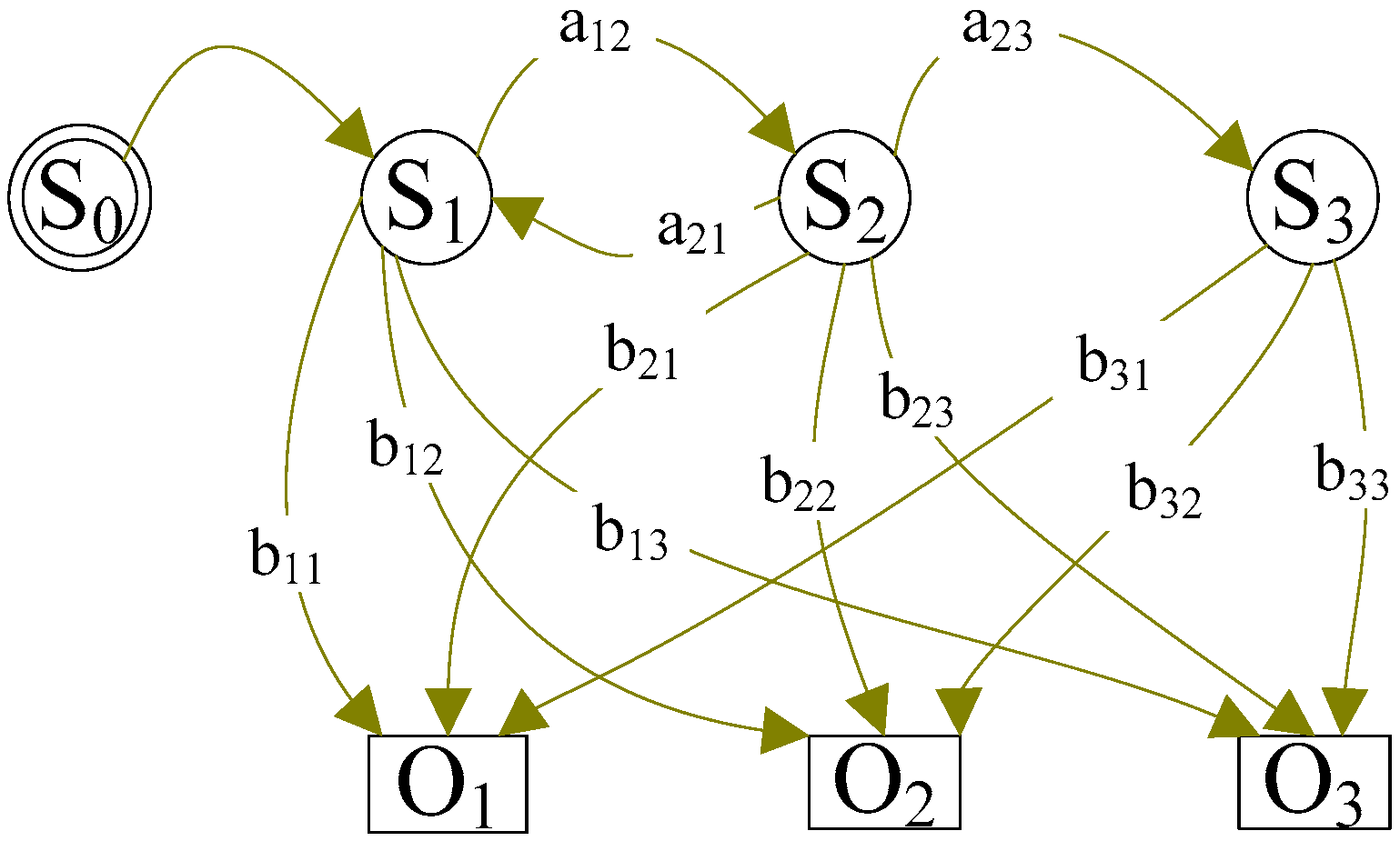
The object of a HMM is to model the state sequence over time. The state space for a HMM model includes a finite set of states, each of which is associated with a probability distribution. The transitions among these states are governed with a certain probability which is referred as state transition probability. In any state, an observation can be generated with certain probability, which was called emission probability. However, the actual state is not externally visible, which explains the appellation “hidden” Markov model. The general architecture of a HMM is shown in Figure 1.
The architecture has two layers: {St} represents the state vector which reflects all possible states at time t; {Ot} represents the observation at time t, and these layers correspond to the state of the system at time t. describes that a HMM as follows:
(1) State space.
State space defines the possible states in the model, which are represented as V. Although the states are hidden, a certain map function exists between the state and the observation. State space is described as a 1 × N vector (N is the number of states in the model). The state of the system qt at time t belongs to V, that is to say, .
(2) Observations.
The observation symbols correspond to the output of the system that is being modeled under a certain map function. Observations are described as a 1 × M vector (M is the number of observations in the model). Observation ot denotes the observation of the system at time t.
(3) State transition probability.
The state transition probability matrix shows probability when the state transit from one state to another state. State transition probability is described as a N × N matrix, such as A = {aij}. aij is the value of the i-th row and the j-th column in the N × N matrix, which shows the probability when the system transits from state Vi to state Vj.
(4) Emission probability.
The emission probability indicates the observation probability distribution in state qt of the system at time t. Emission probability is described as an N × M matrix, such as B = {}. reflects the probability when the system is in state Vi, that observation of the system is oj at time j.
(5) Initial state distribution.
Usually, the initial state in HMM is expressed as π.
where Vτ is the true initial state of the system
A complete specification of a HMM requires specification of the two model parameters (N and M), specification of the observation symbols and the specification of the three probability measures A, B and π. For convenience, we use the compact notation as follows:
3.2. Basics of Viterbi Algorithm
The Viterbi Algorithm [39] is a recursive programming algorithm for finding the most likely sequence of hidden states—the Viterbi path that results in a sequence of a discrete-time finite-state Markov process.
In a HMM, the state is not directly visible, however variables influenced by the state are visible. Each state has a probability distribution over the possible observations. The state of the system mutates from one state to another with a certain probability described by the state transition probability. Meanwhile, estimated locations (GPS measurement or other mobile positioning results) are the visible observation layer and correct road links are the invisible state layer. The vehicle moves on road links from one to another during certain time period with certain probability. Given the characters of the map-matching and HMM model, we applied the Viterbi algorithm to estimate the sequence of road links based on observed GPS positions in this study.
Let denotes the observation (i.e., a GPS data point) obtained at time t, for 1 ≤ t ≤ M.
Let denotes the actual state of the system (i.e., road link in which the system locates) at time t, for 1 ≤ t ≤ M.
Suppose there are N states in the state space, representing N candidate road links. The observation sequence has M observations when the time ranges from 1 to M. The transition probability from any time i to the next time j represent the probability of the system moving from one road link to another. The objective is to find the actual road links sequence , that has maximum probability given the observations. Thus is maximized.
Based on the conditional probabilities from probability theory, for any sequence {q1 … qt}, when qi and qj (1 ≤ i, j ≤ N) are independent.
The denominator of Equation (6) depends only on the observations, but is not dependent on the path . Given that the observation, is determined, even the exact value of the expression is unknown, that is:
Given the condition that qi and qj (1 ≤ i, j ≤ N) are independent, then oi and oj (1 ≤ i, j ≤ N) are independent, and using the probability theory, MAX{P(q1 … qt … qm, o1 … ot … om)} transform as follows:
Within the HMM, the state of the system at time t, depends only on the state of system as time t − 1, but is not related to states or observations prior to the previous state, that is:
And the observation at time t only depends on the state of system as time t, but not relate to previous states or observations. That is to say:
By substituting Equations (9) and (10) into Equation (8), the computable formula can be obtained as follows:
The actual path that fits Equation (11) within the HMM model above can be obtained using the Viterbi algorithm.
3.3. HMM-Based Map-Matching
The HMM-based map-matching algorithm models the map-matching process with the Markov process. Figure 2 shows the map-matching process with HMM. State space in HMM-based map-matching is a set of candidate road links near the GPS data and mobile phone data. S0 is the initial state distribution of the system, St is the state vector and qt is the real state of the system (even it is not seeable), at time t. When the state transforms from qi to qj, the rule is defined in a state transition probability matrix. States of the system are not externally visible during the process, but one outcome is derived from each state with a certain probability, which is referred to as emission probability. This section formulates the parameters to define the HMM for map-matching with GPS data and mobile phone data.
State space. In HMM-based map-matching, the state of the system which consists of road links, is set to R1, R2, … Rn. All road links in the road network are structured with a quad-tree grid. Thus, when the GPS data and the mobile phone data are confirmed, the grid in which these data are located can be obtained. Road links in these grids compose the state space in HMM model.
Observations. The observation symbols correspond to the output of the system that is being modeled for a certain map function. The observations are distinct, and include GPS data and mobile phone data.
State transition probability. The state transition probability matrix reflects probability when the state transits from one state to another state. In the map-matching process, a vehicle moves on one road link to the road link that is connected (before or after) with the previous road link. Topology of the network should be considered when defining the state transition probability. Considering the length of the road links and the maximum vehicle speed, the probability of moving on one road link to the next road link depends on the length of the road links.
Considering the vehicle speed and the time interval, movement on the road link, which is far away from the road link at this moment is not possible. This information indicates that the mean length of road link is 119 m and the average distance between two successive estimated positions is 21 m, the vehicle moves on the same road link with a possibility of 3/5 (i.e., the approximate value of (119 – 21 × 2)/119).
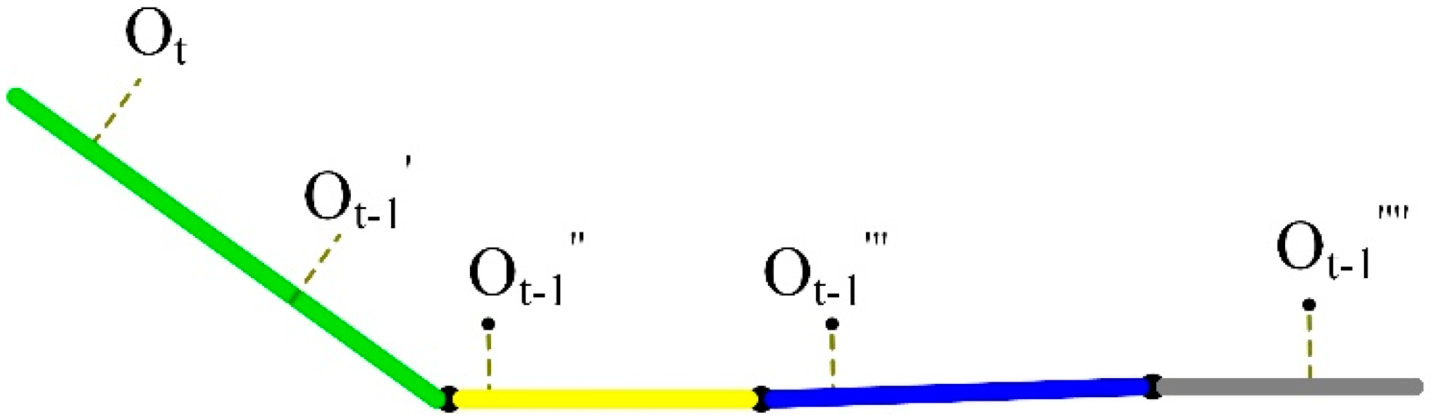
Figure 3 indicates the possibility of the next state given the current state. Given the state at time t, the next state can be the same road link (marked with green), or the road link which is a directly connected road link (marked with yellow), or the road link which is separated from the previous state by only one road link (marked with blue), but not the road link which is far from the previous state (marked with gray).
The state transition probability (aij in state transition matrix) in HMM-based map-matching in this work, depends on the connectivity among the road link in road network. It is defined with the rules as follows:
Emission probability means the observation probability distribution in each state qt at time t. Based on the basic geospatial analysis that event A is assigned with a greater reward to point P for being ‘closer’ to point P [37], it is reasonable to say that the shorter the project distance from one observation to nearby road links is, the greater the probability of being the true state for the observation. Here this work takes the connectivity information of the road network to calculate emission probability, with rules in Equation (12). Figure 4 shows a simplified road network to illustrate of state transition matrix. Table 1 illustrates the state transition matrix for road network in Figure 4.
For each observation, we calculate the distance between the observation and the road links in state space. The road links within a certain distance to the observation is selected to perform this calculation and eliminates the computation complexity in the Viterbi algorithm.
The ri … rk are road links which are far from ot within a certain distance. A statistical analysis of the data indicate that the maximal distance between successive two points is less than 80 m, and mean distance is 18.96 m. Considering the previous experience about the accuracy of GPS data and road networks, the threshold value for the distance between two road links is 80 m.
The initial probability distribution S0, as shown in Figure 2, shows the initial value for the iterative computation in the Viterbi algorithm. To improve the universality of the HMM-based map-matching, we create the initial state distribution by selecting the road links near the first 10 GPS points. Road links in this set are equally assigned with probability 1/k when k is the number of road links in this set.
3.4. Process
Figure 5 shows the processes in HMM-based map-matching for GPS data and mobile phone data. First, the state space for the HMM is obtained by selecting road links within a certain distance to all GPS data. Second, the initial state probability distribution is confirmed by assigning the road links near the first GPS point within a certain distance with probability 1/k when k is the number of road links in this set. Thirdly GPS data is read as observations. With geometric information between GPS data (observation) and road links (state), the emission probability matrix can be generated considering the shortest distance between each GPS datum and to each road links within certain a distance. With the topology among the road links (state), state transition probability matrix can be generated with the rule in Section 3.3. With these well-defined parameters, the Viterbi algorithm generates the Viterbi path that is the hidden state sequence with the maximum probability. Each GPS datum corresponds to one road link and these road links are directly connected. Not all road links are connected together, because the majority of the GPS data are projected to long road links, but not short road links in the road network. After we analyze the characteristics of the road links in the network, the missing road links can be obtained by selecting the links connected with road links in the Viterbi path. Finally a map-aiding operation is performed to inquire about missing road links related to the Viterbi path, eliminate superfluous road links, reconnect the road links and obtain the map-matching results.
4. Experiment and Analysis
To test the HMM-based map-matching, we take four set of data to validate the algorithm: two sets of GPS data and two sets of A-bis interface data from a cellular network in the Do-iT project [7]. The road links on the road network are classified into three levels.
4.1. Map-Matching with HMM on GPS Positioning
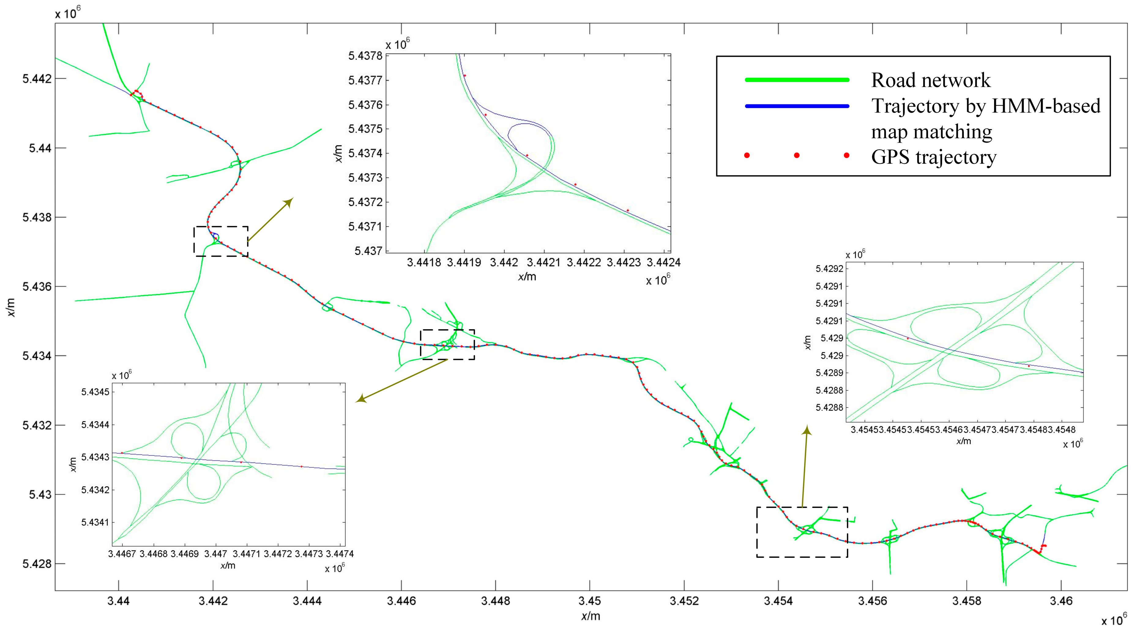
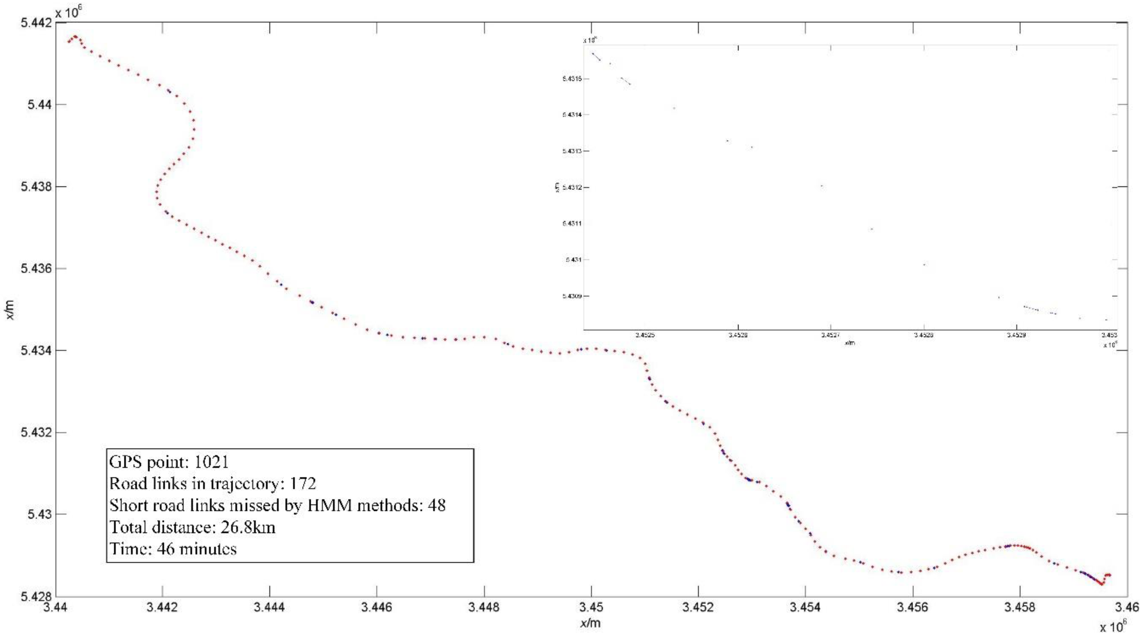
The first test deals with a set of GPS data with approximate 28 km along its trajectory. Sample rate of the data is 0.5 Hz. Figure 6 shows the visualization of the Viterbi path, which is represented by blue links. A statistical analysis indicates that the HMM-based map-matching have high efficiency and accuracy than other map-matching methods. At the same time, certain road links which do not belong to the true trajectory were also selected, only because the project distance from a GPS point to these road links is shorter. Short road links are missed because the project distance from the GPS point to these links is longer than the project distance between the GPS points and their neighbors. The visualization of these missing short road links and the GPS points nearby is shown in Figure 7. Map-aiding operation aims to query regarding missing road links related to the Viterbi path, eliminate superfluous road links, reconnect the road links and get the map-matching result. This approach improves the results from the Viterbi algorithms; details are visualized in Figure 8.
4.2. Map-Matching with HMM in Large Scale Road Network
The second set of experimental data is a GPS data in large scale road network from Microsoft public data [35] (Figure 9a), with a 1 Hz sample rate. Figure 9 shows the procedures to select the candidate road links for map-matching with a HMM. After obtaining the minimal boundary box of all road links, road links near the GPS area can be easily obtained by comparing the boundary (Figure 9b). Then we build a local quad-tree structure, and GPS point and road links nearby are marked with a grid ID. Then road links with grid ID at which the GPS point is located are selected (Figure 9c). The time to generate emission probability is reduced by 50% after exploiting the Quad-tree structure. Considering the GPS signal blockage, we detect the area where GPS signal blockage happens, by checking the interval distance inside of GPS trajectory, and obtain the grid ID and road links near these areas (Figure 9d). Then we create five parameters for the HMM model and use the Viterbi algorithm to generate the Viterbi path for the GPS trajectory. Finally we perform a map-aiding operation to acquire missing road links, eliminate superfluous road links, reconnect the road links in the Viterbi path and obtain the map-matching results. This improves the results from the Viterbi algorithms, and enhances the correct rate to exceed 98.6%.
Figure 10 shows the global results of the HMM-based map matching method and details of several tiny “limitations”, with corresponding GPS trajectories. Although the road map covers 200 km × 120 km, the algorithm obtains minimal data set that encompasses the GPS trajectory, by cutting the road map with grids. Road links calculated are not totally connected along the GPS trajectory. Some road links which do not belong to the real trajectory, are referred in the preliminary result. Within the area of tiny “limitations”, we do not observe any GPS point data, which are marked as green points. By comparing the road map with Google Map, we observe a tunnel and deduce that GPS signal was blocked when the GPS receiver passed through this area.
After analyzing the reasons for tiny “limitations” and short links linked with the object route, the methods were improved by map-aiding operation, which includes two steps. The first step is to connect all selected links despite a gap due to the missing GPS points. By calculating the distance between two successive GPS points and the length of the road links, we deduce that links at “limitations” area in the initial result are less than four links, which can be easily acquired by selecting links that are linked with the previous set of road links and repeated one time. The second step is to get rid of redundant road links around the true trajectory by calculating the refined road network again with HMM model. The details of Figure 11 show the result of HMM-based map-matching operation with map-aiding operation. Details in Figure 11 show the improvement of the HMM-based map matching with the map-aiding operation compared with Figure 10.
4.3. Map-Matching with HMM on Low-Rate Positioning Data
The third set of experimental data is a set of low-rate GPS data (0.2 Hz sample rate), which is obtained by rarefying the second set in Section 4.2. The sequence of map-matching based on HMM on low-rate GPS data is same to that in Section 4.2, including: (a) to rebuild the road network data with the quad-tree structure, (b) to add a new mark to the road links and GPS points to link the road and GPS points with the Quadtree code, (c) to build the HMM model with obtained data and generate the Viterbi path for the rarefied GPS trajectory, (d) to calculate the new parameters for the subsequent map-aiding operation.
The difference between these experiments are the parameters to generate the state space and state transition probability (because observations is the low-rate GPS data). The parameters are dependent on the features of observations, like longest distance between two successive points and the length of minimal boxing boundary.
As a result, the direct output by map-matching with the Markov model and Viterbi algorithms consists of the true road trajectories from the road network links, with the correct rate of 96.9%, and this rate is further improved by the following map-aiding operation.
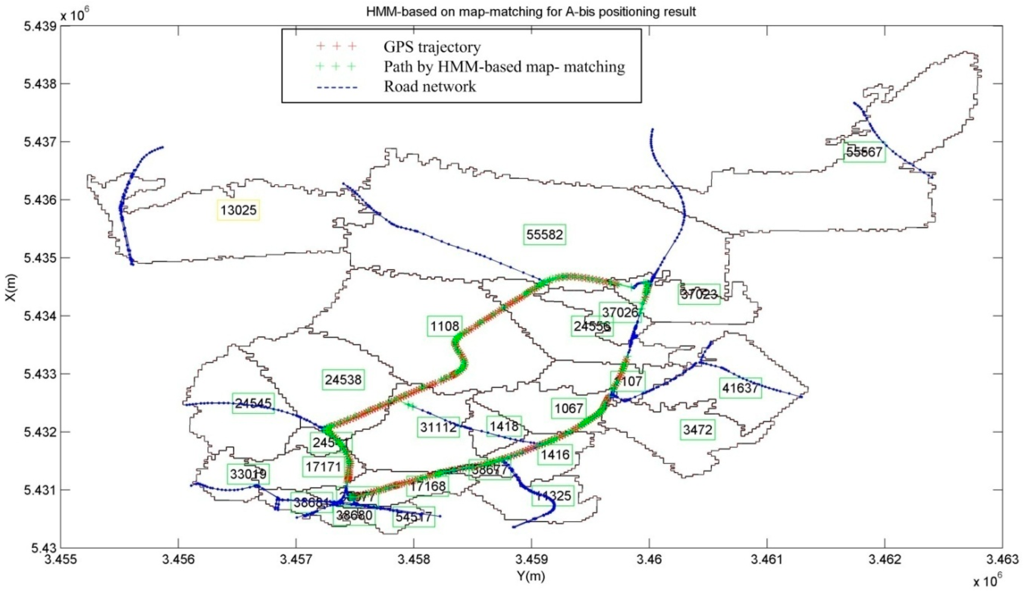
4.4. Map-Matching with HMM on Mobile Phone Positioning with Signal Strength
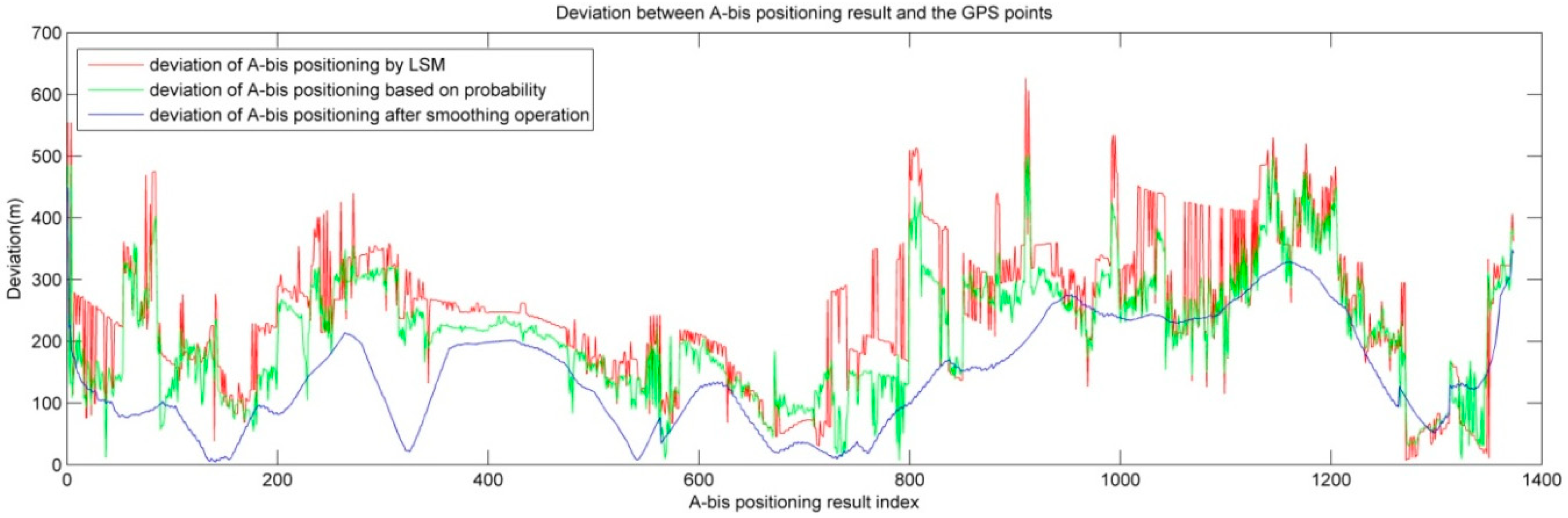
Mobile phone positioning by received signal strength matching is still with accuracy of 60–120 m in most existing applications [7]. The majority of existing map-matching methods cannot generate promising results for estimated locations with this level of accuracy. Figure 12 shows the positioning accuracy about the mobile positioning result by A-bis data from GSM network system (Sample rate is 0.5 Hz).
The HMM-based map-matching algorithm calculates the possibility of each possible path, and outputs the state at each epoch.
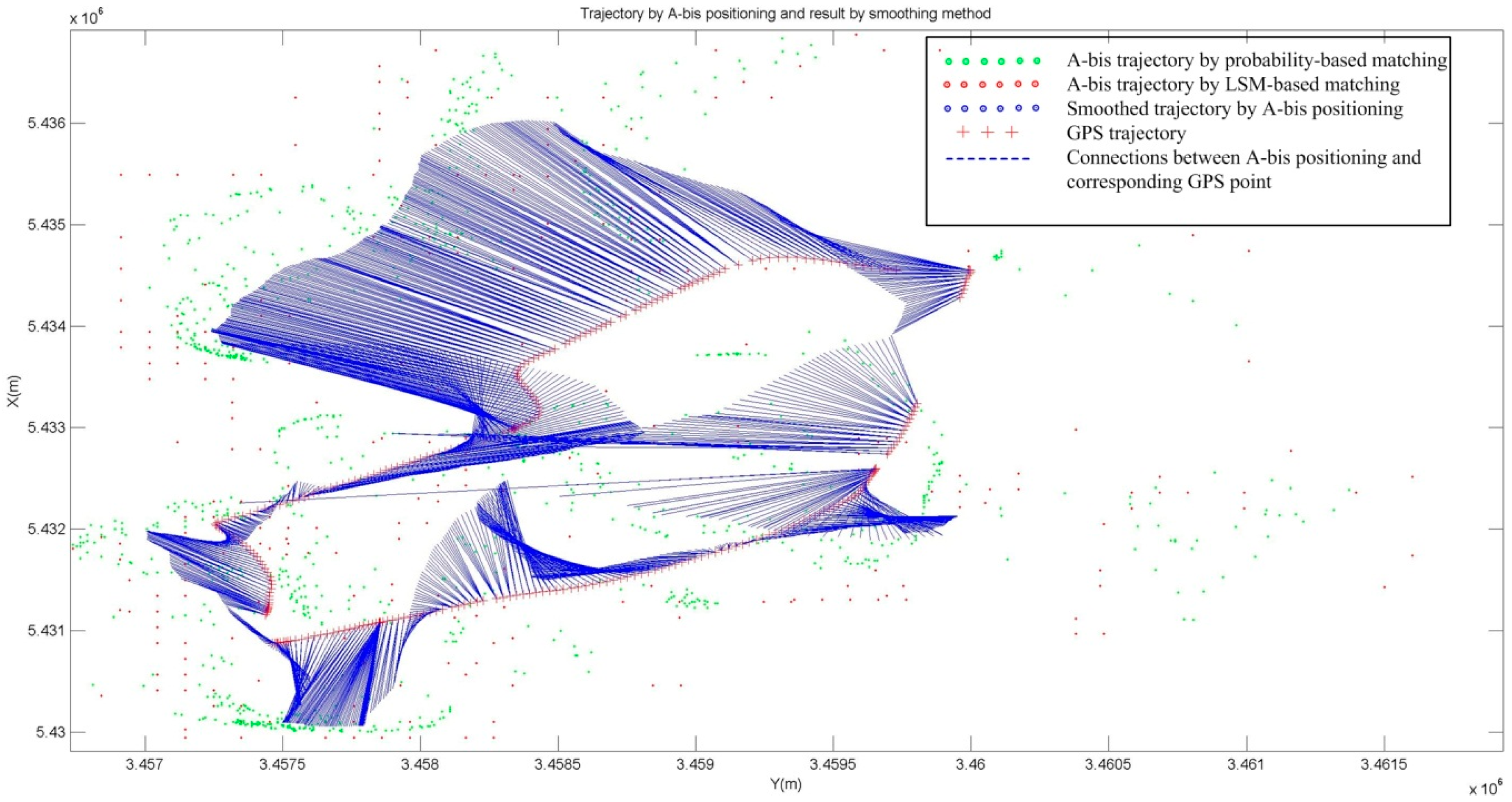
Regarding mobile phone positioning, the raw results are not as accurate as GPS positioning in most cases. Figure 13 shows the raw A-bis data positioning and the results refined using the smoothing method.
With the similar steps to do map matching with the HMM model, result from A-bis data positioning can be well matched with road network, as shown in Figure 14.
4.5. Summary of the Validation
Totally, we employ with four set of data to validate the HMM-based map-matching algorithm. Table 2 provides an overview of the performance about these tests. Two aspects are particularly notable. The first aspect is that the maximum average correct rate with HMM-based map-matching is 97.2%. This correct rate shows that the HMM is valid for map-matching process whatever the sampling rate, and accuracy of raw positioning data. It is a remarkable contrast to the temporary result during the process. The second aspect is that the results from HMM-based map-matching on GPS data achieve a higher correct rate, than that of mobile phone positioning. The reason for this is that the accuracy of GPS is significantly higher than the accuracy of the positioning by A-bis data from the cellular phone system. Thus, the road links at the start and end part of trajectory cannot be matched. The result from GPS data route 4 and shows that HMM-based map-matching algorithm proposed in this work can obtain a stable map-matching result, even with positioning data with low sampling rate (0.1 Hz).
We propose methods to improve the algorithm efficiency by reducing the order of complexity. When road links in the network are structured with appropriate quad-tree structure, the efficiency is significantly improved. The optimal side length of the basic square in the quad-tree structure depends on the mean projection distance between the observations and the road links, the mean road links in network.
Another aspect is related to the generation of the state transition probability and the emission probability. For a normal HMM, the transition probability from one state to any other state in the state space should be separately calculated from the emission probability from the state to the observation at each time slot. In HMM-based map-matching, topological and geometric information of the road network were considered to enhance the generation of the HMM. With network topological information, possible states for the specific observation can be calculated by searching the road links with certain distance from the observation. In this study the time complexity in the Viterbi algorithm is reduced from to the more favorable .
5. Conclusions
We present a HMM-based map-matching algorithm for GPS positioning and mobile phone positioning. The algorithm employs geometric information, topology matrix of the road network and relativity between the positioning points and the candidate links, when describing the Markov process, and algorithms to find the Viterbi path with highest probability. The experiment results demonstrate that the HMM-based map-matching algorithm significantly improves the algorithm efficiency in terms of accuracy. Even the sampling rate of the positioning data is changed to 0.1 Hz (average distance for successive two points is about 200 m.), the quad-tree data structure and topology relationship model significantly narrow the computing space. Map-aiding with topology information and features of road network links has significant importance in exploiting the use of HMM-based map-matching methods. Low frequency observations can also be matched with high accuracy when topological information is exploited to generate the state transition probability.
In order to further improve the efficiencies and suitability of the HMM-based map-matching method, more features should be reviewed. Most map-matching algorithms, including the HMM-based map-matching in this work, take the following condition: “the vehicle can only turn onto legal road segments”. However, this condition is not right all the time. Another topic is timeliness. The HMM-based map-matching works very well, in terms of long-term time span. When in the early period of a map-matching work, number of observations and degree of state transition matrix are still small at the beginning. This will lead to a significant matching deviation. In future research work, we are interested in developing matching method to address these problems.
Acknowledgments
This work was supported by the National Key Research and Development Program of China (No. 2017YFB0503502, 2017YFB0503601).
Author Contributions
An Luo and Shenghua Chen designed the research and wrote the paper, Shenghua Chen and Bin Xv analyzed the data and performed the research, An Luo and Shenghua Chen co-designed the research and extensively updated the paper. All authors read and approved the final manuscript.
Conflicts of Interest
The authors declare no conflict of interest.
References
- Bierlaire, M.; Chen, J.; Newman, J. A probabilistic map matching method for smartphone GPS data. Transp. Res. Part C Emerg. Technol. 2013, 26, 78–98. [Google Scholar] [CrossRef]
- Griffin, T.; Huang, Y.; Seals, S. Routing-based map matching for extracting routes from GPS trajectories. In Proceedings of the 2nd International Conference on Computing for Geospatial Research & Applications, Washington, DC, USA, 23–25 May 2011; p. 24. [Google Scholar]
- Kainz, W.; Christ, A.; Kellom, T.; Seidman, S.; Nikoloski, N.; Beard, B.; Kuster, N. Dosimetric comparison of the specific anthropomorphic mannequin (SAM) to 14 anatomical head models using a novel definition for the mobile phone positioning. Phys. Med. Biol. 2005, 50, 3423. [Google Scholar] [CrossRef] [PubMed]
- Katrin, R.; Volker, S. Mobile positioning for traffic state acquisition. J. Locat. Based Serv. 2007, 1, 133–144. [Google Scholar]
- Dalumpines, R.; Scott, D.M. GIS-based map-matching: Development and demonstration of a post processing map-matching algorithm for transportation research. In Advancing Geo-Information Science for a Changing World; Springer: Berlin/Heidelberg, Germany, 2011; pp. 101–120. [Google Scholar]
- Zhou, X.; Liu, J.; Yeh, A.G.O.; Yue, Y.; Li, W. The Uncertain Geographic Context Problem in Identifying Activity Centers Using Mobile Phone Positioning Data and Point of Interest Data. In Advances in Spatial Data Handling and Analysis; Springer International Publishing: Basel, Switzerland, 2015; pp. 107–119. [Google Scholar]
- Wiltschko, T.; Schwieger, V.; Möhlenbrink, W. Generating Floating Phone Data for Traffic Flow Optimization. In Proceedings of the 3rd International Symposium “Networks for Mobility”, Stuttgart, Germany, 5–6 October 2006. [Google Scholar]
- Hu, J.; Cao, W.; Luo, J.; Yu, X. Dynamic modeling of urban population travel behavior based on data fusion of mobile phone positioning data and FCD. In Proceedings of the 2009 17th International Conference on Geoinformatics, Fairfax, VA, USA, 12–14 August 2009; pp. 1–5. [Google Scholar]
- Quddus, M.; Ochieng, W.; Noland, R. Current map-matching algorithms for transport applications: State-of-the art and future research directions. Transp. Res. Part C Emerg. Technol. 2007, 15, 312–328. [Google Scholar] [CrossRef] [Green Version]
- Pink, O.; Hummel, B. A statistical approach to map-matching using road network geometry, topology and vehicular motion constraints. In Proceedings of the 11th International IEEE Conference on Intelligent Transportation Systems, Beijing, China, 12–15 October 2008; pp. 862–867. [Google Scholar]
- Weil, M. Drafting a new route planning system: Molson Coors Canada’s new delivery planning system taps routing, pallet building, and truck loading functionality to optimize shipment flow. Inbound Logist. 2014, 34, 293–296. [Google Scholar]
- Mahdi, H.; Hassan, A.K. A critical review of real-time map-matching algorithms: Current issues and future directions. Comput. Environ. Urban Syst. 2014, 48, 153–165. [Google Scholar]
- Yoonsik, B.; Jiyoung, K.; Kiyun, Y. An Improved Map-Matching Technique Based on the Fréchet Distance Approach for Pedestrian Navigation Services. Sensors 2016, 16, 1768. [Google Scholar] [CrossRef]
- Felipe, J.; Sergio, M.; Jose, E.N. Definition of an Enhanced Map-Matching Algorithm for Urban Environments with Poor GNSS Signal Quality. Sensors 2016, 16, 193. [Google Scholar] [CrossRef]
- Qinglin, T.; Zoran, S.; Kevin, I.W. A Hybrid Indoor Localization and Navigation System with Map Matching for Pedestrians Using Smartphones. Sensors 2015, 15, 30759–30783. [Google Scholar] [CrossRef]
- Sylvie, L.-P.; Nicolas, G.; Mehdi, B. A HMM map-matching approach enhancing indoor positioning performances of an inertial measurement system. In Proceedings of the International Conference on Indoor Positioning and Indoor Navigation, Banff, AB, Canada, 13–16 October 2015; pp. 1–4. [Google Scholar]
- Jagadeesh, G.R.; Srikanthan, T.; Zhang, X.D. A Map-matching Method for GPS Based Real-Time Vehicle Location. J. Navig. 2004, 57, 429–440. [Google Scholar] [CrossRef]
- Quddus, M.A.; Noland, R.B.; Ochieng, W.Y. Validation of map-matching algorithm using high precision positioning with GPS. J. Navig. 2004, 58, 257–271. [Google Scholar] [CrossRef]
- Jagadeesh, G.R.; Srikanthan, T. Probabilistic Map Matching of Sparse and Noisy Smartphone Location Data. In Proceedings of the 2015 IEEE 18th International Conference on Intelligent Transportation Systems, Las Palmas, Spain, 15–18 September 2015; pp. 812–817. [Google Scholar]
- Meng, Y. Improved Positioning of Land Vehicle in ITS Using Digital Map and Other Accessory Information. Ph.D. Thesis, Department of Land Surveying and Geoinformatics, Hong Kong Polytechnic University, Hong Kong, China, 2006. [Google Scholar]
- Quddus, M.A.; Ochieng, W.Y.; Zhao, L.; Noland, R.B. A general map-matching algorithm for transport telematics applications. GPS Solut. 2003, 7, 157–167. [Google Scholar] [CrossRef] [Green Version]
- Taylor, G.; Brunsdon, C.; Li, J.; Olden, A.; Steup, D.; Winter, M. GPS accuracy estimation using map-matching techniques: Applied to vehicle positioning and odometer calibration. Comput. Environ. Urban Syst. 2006, 30, 757–772. [Google Scholar] [CrossRef]
- Ren, M.; Karimi, H.A. A hidden Markov model-based map-matching algorithm for wheelchair navigation. J. Navig. 2009, 62, 383–395. [Google Scholar] [CrossRef]
- Ochieng, W.Y.; Quddus, M.A.; Noland, R.B. Map-matching in complex urban road networks. Rev. Bras. Cartogr. 2003, 5, 1–18. [Google Scholar]
- Chen, B.Y.; Yuan, H.; Li, Q.; Lam, W.H.; Shaw, S.L.; Yan, K. Map matching algorithm for large-scale low-frequency floating car data. Int. J. Geogr. Inf. Sci. 2014, 28, 22–38. [Google Scholar] [CrossRef]
- Krakiwsky, E.J.; Harris, C.B.; Wong, R.V.C. A Kalman filter for integrating dead reckoning, map matching and GPS positioning. In Proceedings of the IEEE PLANS’ 88—Position Location and Navigation Symposium Record: Navigation into the 21st Century, Orlando, FL, USA, 29 November–2 December 1988; pp. 39–46. [Google Scholar]
- Pyo, J.S.; Shin, D.H.; Sung, T.K. Development of a map matching method using the multiple hypothesis technique. In Proceedings of the 2001 IEEE Intelligent Transportation Systems, Oakland, CA, USA, 25–29 August 2001; pp. 23–27. [Google Scholar]
- Yuan, J.; Zheng, Y.; Zhang, C.; Xie, X.; Sun, G.Z. An interactive-voting based map matching algorithm. In Proceedings of the 2010 Eleventh International Conference on Mobile Data Management, Kansas City, MO, USA, 23–26 May 2010; pp. 43–52. [Google Scholar]
- Toledo-Moreo, R.; Bétaille, D.; Peyret, F. Lane-level integrity provision for navigation and map matching with GNSS, dead reckoning, and enhanced maps. IEEE Trans. Intell. Transp. Syst. 2010, 11, 100–112. [Google Scholar] [CrossRef]
- Shin, S.H.; Park, C.G.; Choi, S. New map-matching algorithm using virtual track for pedestrian dead reckoning. ETRI J. 2010, 32, 891–900. [Google Scholar] [CrossRef]
- Sajid, S.; Geoff, G.; Andrew, M. Fast State Discovery for HMM Model Selection and Learning. In Proceedings of the Eleventh International Conference on Artificial Intelligence and Statistics (AI-STATS), San Juan, Puerto Rico, 21–24 March 2007. [Google Scholar]
- Raymond, R.; Morimura, T.; Osogami, T.; Hirosue, N. Map-matching with hidden Markov model on sampled road network. In Proceedings of the 2012 21st International Conference on Pattern Recognition (ICPR), Tsukuba, Japan, 11–15 November 2012; pp. 2242–2245. [Google Scholar]
- Newson, P.; Krumm, J. Hidden Markov map matching through noise and sparseness. In Proceedings of the 17th ACM SIGSPATIAL International Conference on Advances in Geographic Information Systems, Seattle, WA, USA, 4–6 November 2009; pp. 336–343. [Google Scholar]
- Yin, H.; Wolfson, O. A weight-based map matching method in moving objects databases. In Proceedings of the 16th International Conference on Scientific and Statistical Database Management, Santorini Island, Greece, 23 June 2004; pp. 437–438. [Google Scholar]
- Lou, Y.; Zhang, C.; Zheng, Y.; Xie, X.; Wang, W.; Huang, Y. Map-matching for low-sampling-rate GPS trajectories. In Proceedings of the 17th ACM SIGSPATIAL International Conference on Advances in Geographic Information Systems, Seattle, WA, USA, 4–6 November 2009; pp. 352–361. [Google Scholar]
- Wang, Y.; Zhu, Y.; He, Z.; Yue, Y.; Li, Q. Challenges and Opportunities in Exploiting Large-Scale GPS Probe Data; Technical Report HPL-2011-109; HP Laboratories: Palo Alto, CA, USA, 2011. [Google Scholar]
- Paulo, S.; John, P.D. Adversarial Geospatial Abduction Problems. ACM Trans. Intell. Syst. Technol. 2012, 3, 1–35. [Google Scholar]
- Yankai, L.; Zhou, L. A novel algorithm of low sampling rate GPS trajectories on map-matching. J. Wirel. Commun. Netw. 2017, 2017, 30. [Google Scholar] [CrossRef]
- Forney, G.D. The Viterbi algorithm. Proc. IEEE 1973, 61, 268–278. [Google Scholar] [CrossRef]
- Viterbi, A.J. Error bounds for convolutional codes and an asymptotically optimum decoding algorithm. IEEE Trans. Inf. Theory 1967, 13, 260–269. [Google Scholar] [CrossRef]
- Lawrence, R.R. A Tutorial on Hidden Markov Models and Selected Applications in Speech Recognition. Proc. IEEE 1989, 77, 257–287. [Google Scholar]
- Szwed, P.; Pekala, K. An Incremental Map-Matching Algorithm Based on Hidden Markov Model. In Proceedings of the 13th International Conference Artificial Intelligence and Soft Computing Volume 8468 of the Series Lecture Notes in Computer Science, ICAISC 2014, Zakopane, Poland, 1–5 June 2014; pp. 579–590. [Google Scholar]
- Xia, Y.; Liu, Y.; Ye, Z.; Wu, W.; Zhu, M. Quadtree-based domain decomposition for parallel map-matching on GPS data. In Proceedings of the 2012 15th International IEEE Conference on Intelligent Transportation Systems, Anchorage, AK, USA, 16–19 September 2012; pp. 808–813. [Google Scholar]
- Oran, A.; Jaillet, P. An HMM-based map matching method with cumulative proximity-weight formulation. In Proceedings of the 2013 International Conference on Connected Vehicles and Expo (ICCVE), Las Vegas, NV, USA, 2–6 December 2012; pp. 480–485. [Google Scholar]
Figure 1.
Hidden Markov Model (HMM) with its five parameters.

Figure 2.
Modeling the map-matching with HMM.
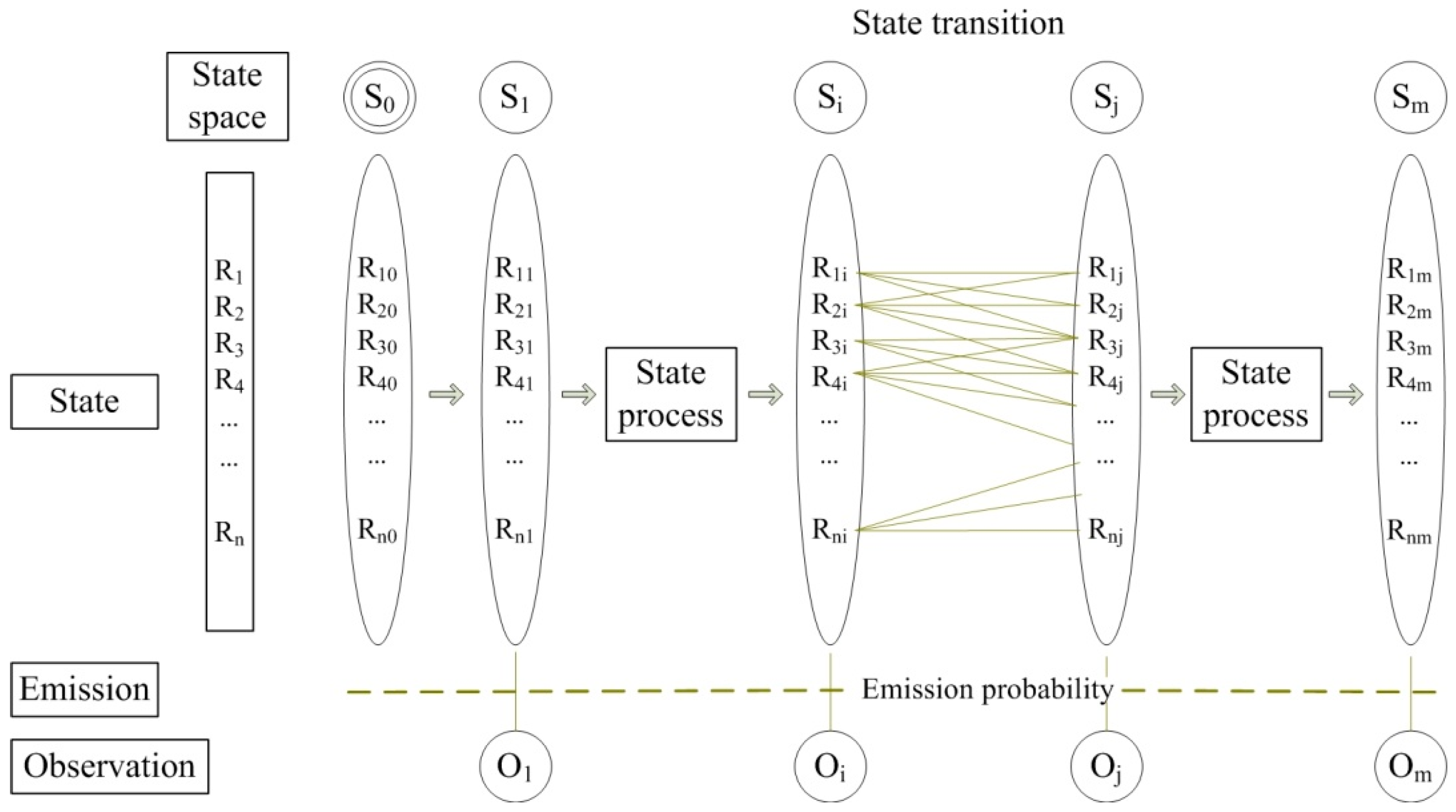
Figure 3.
State transit based on the network connectivity.

Figure 4.
Simplified road network to illustrate of state transition matrix.
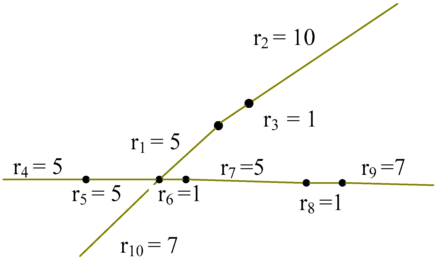
Figure 5.
Processes in HMM-based map-matching.
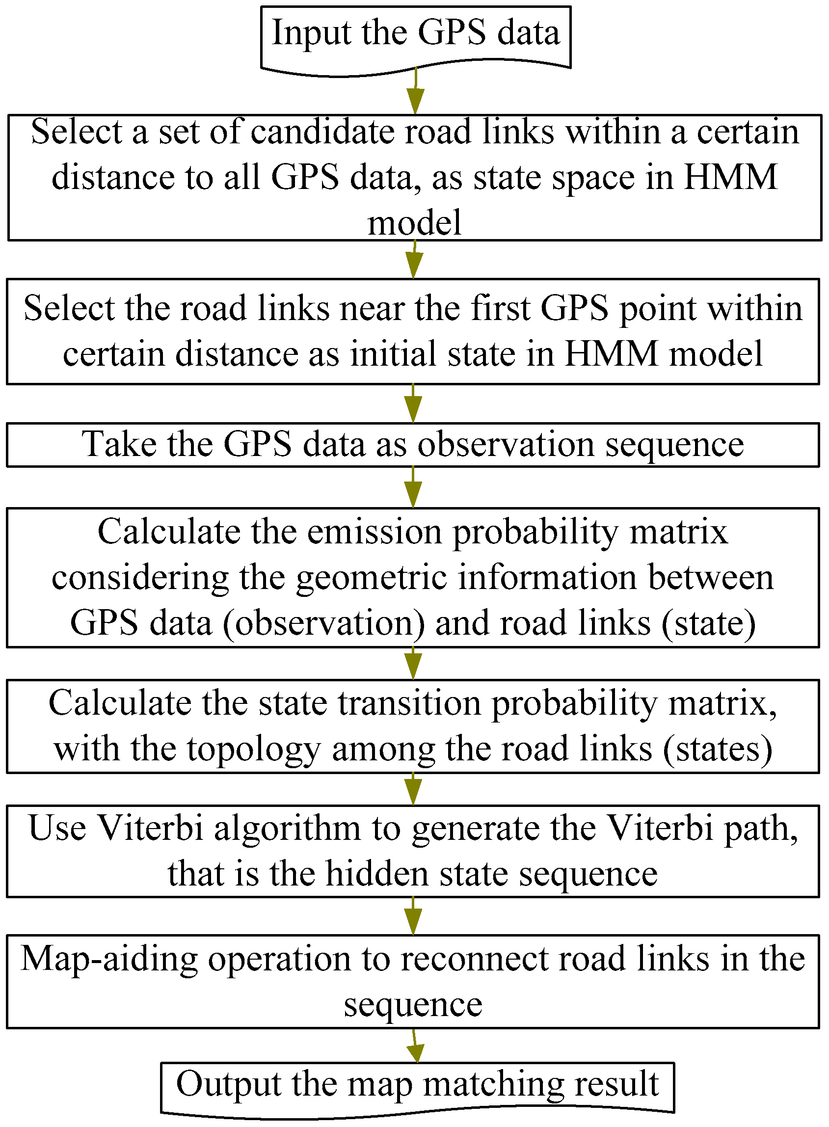
Figure 6.
Details of the Viterbi path in the HMM-based map-matching method.

Figure 7.
Visualization of these missing short road links and the GPS points.
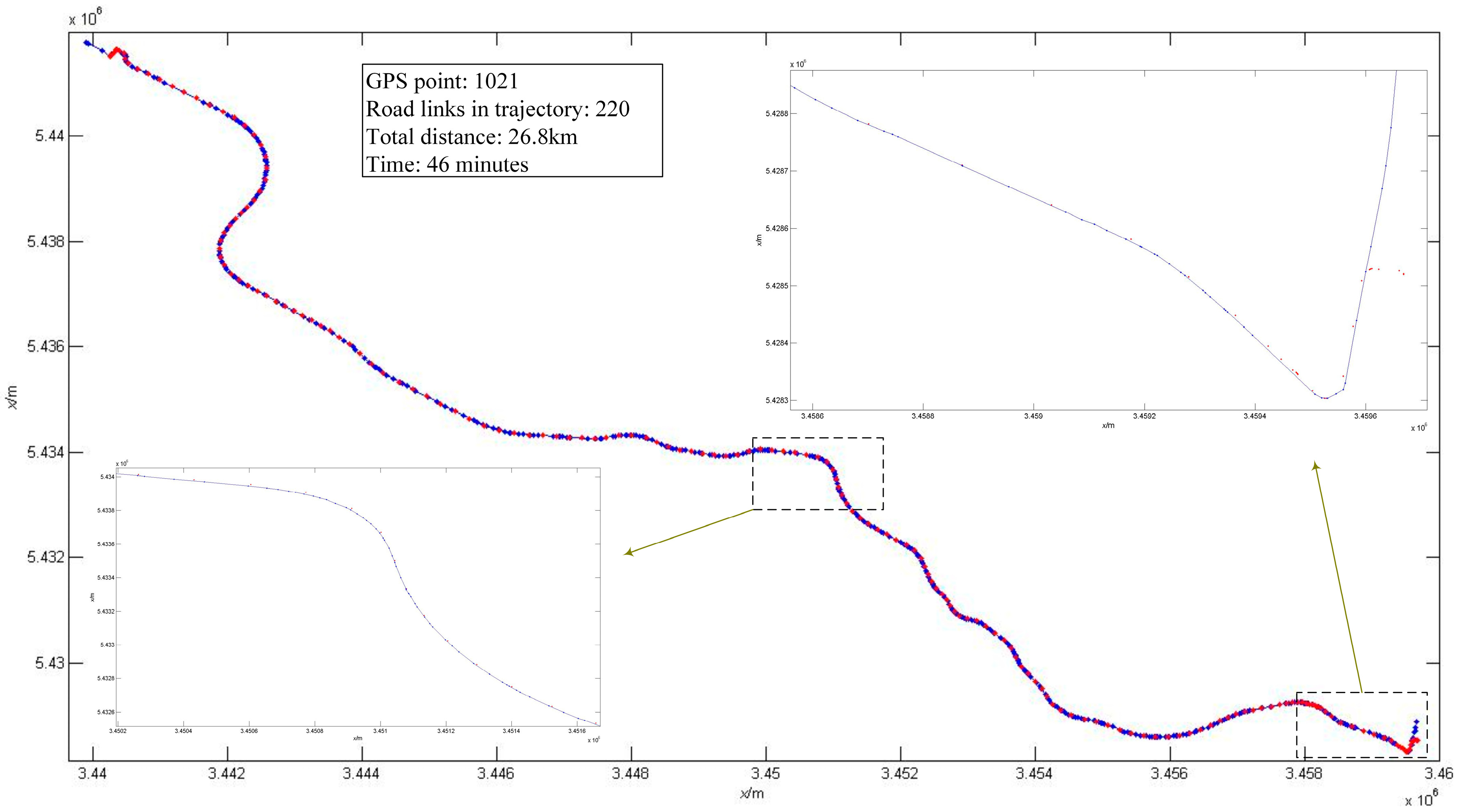
Figure 8.
The improved results from Viterbi algorithms.

Figure 9.
Procedures for map-matching with HMM.

Figure 10.
Result of the HMM-based map-matching method and the GPS trajectory.
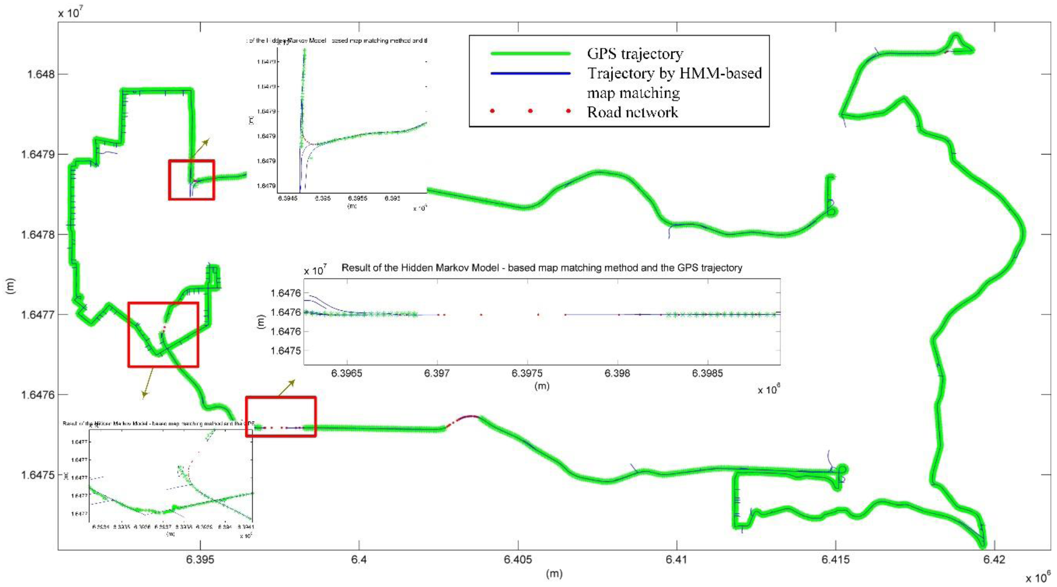
Figure 11.
Result of HMM-based map-matching operation.
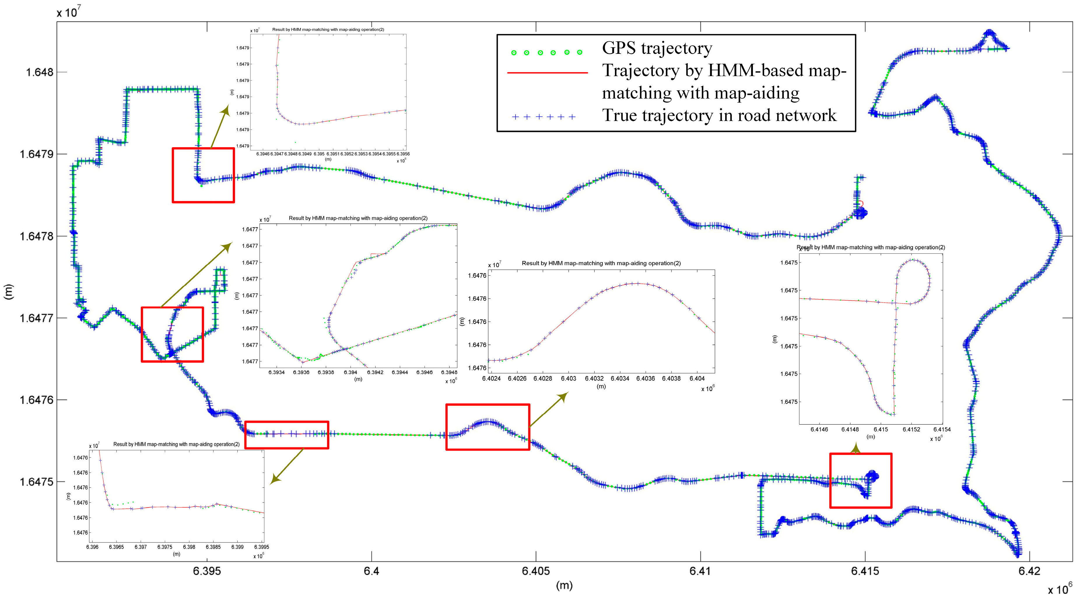
Figure 12.
Deviation between A-bis positioning result and the GPS points.

Figure 13.
Road links in by A-bis positioning and result by smoothing method.

Figure 14.
HMM-based on map-matching for A-bis positioning result.


Table 1.
State transition matrix for road network in Figure 4.
Table 1.
State transition matrix for road network in Figure 4.
| r1 | r2 | r3 | r4 | r5 | r6 | r7 | r8 | r9 | r10 | |
|---|---|---|---|---|---|---|---|---|---|---|
| r1 | 3/5 | 1/5 | 2/5 | 1/5 | 2/5 | 2/5 | 1/5 | 0 | 0 | 2/5 |
| r2 | 1/5 | 3/5 | 2/5 | 0 | 0 | 0 | 0 | 0 | 0 | 0 |
| r3 | 2/5 | 2/5 | 3/5 | 0 | 1/5 | 1/5 | 0 | 0 | 0 | 1/5 |
| r4 | 1/5 | 0 | 0 | 3/5 | 2/5 | 1/5 | 0 | 0 | 0 | 1/5 |
| r5 | 2/5 | 0 | 1/5 | 2/5 | 3/5 | 2/5 | 1/5 | 0 | 0 | 2/5 |
| r6 | 2/5 | 0 | 1/5 | 1/5 | 2/5 | 3/5 | 2/5 | 1/5 | 0 | 2/5 |
| r7 | 1/5 | 0 | 0 | 0 | 1/5 | 2/5 | 3/5 | 2/5 | 1/5 | 1/5 |
| r8 | 0 | 0 | 0 | 0 | 0 | 1/5 | 2/5 | 3/5 | 2/5 | 0 |
| r9 | 0 | 0 | 0 | 0 | 0 | 0 | 1/5 | 2/5 | 3/5 | 0 |
| r10 | 2/5 | 0 | 1/5 | 1/5 | 2/5 | 2/5 | 1/5 | 0 | 0 | 3/5 |
Table 2.
Comprehensive statistical result of all verification test.
| Data Type | Number of Observations | Rate of Short Road Links to Total Trajectories by Length | Correct Rate with HMM after Map Aiding (%) | Trajectory Length (km) |
|---|---|---|---|---|
| GPS data route 1 | 1021 | 1.12% | 100% | 28.6 |
| GPS data route 2 | 7539 | 0.01% | 99.93% | 107.8 |
| A interface data route 3 | 1373 | 1.32% | 95.6% | 26.4 |
| GPS data route 3 | 1373 | 0.51% | 100% | 26.4 |
| A interface data route 4 | 1507 | 1.09% | 95.2% | 31.9 |
| GPS data route 4 | 1507 | 0.39% | 100% | 31.9 |
| GPS data route 4 (low sampling rate) | 301 | 3.64% | 100% | 31.2 |
© 2017 by the authors. Licensee MDPI, Basel, Switzerland. This article is an open access article distributed under the terms and conditions of the Creative Commons Attribution (CC BY) license (http://creativecommons.org/licenses/by/4.0/).
Share and Cite
MDPI and ACS Style
Luo, A.; Chen, S.; Xv, B. Enhanced Map-Matching Algorithm with a Hidden Markov Model for Mobile Phone Positioning. ISPRS Int. J. Geo-Inf. 2017, 6, 327. https://doi.org/10.3390/ijgi6110327
AMA Style
Luo A, Chen S, Xv B. Enhanced Map-Matching Algorithm with a Hidden Markov Model for Mobile Phone Positioning. ISPRS International Journal of Geo-Information. 2017; 6(11):327. https://doi.org/10.3390/ijgi6110327
Chicago/Turabian StyleLuo, An, Shenghua Chen, and Bin Xv. 2017. "Enhanced Map-Matching Algorithm with a Hidden Markov Model for Mobile Phone Positioning" ISPRS International Journal of Geo-Information 6, no. 11: 327. https://doi.org/10.3390/ijgi6110327
Note that from the first issue of 2016, this journal uses article numbers instead of page numbers. See further details here.