Assessment of UAV and Ground-Based Structure from Motion with Multi-View Stereo Photogrammetry in a Gullied Savanna Catchment

 ,
,  , and
, and
Abstract
:1. Introduction
2. Materials and Methods
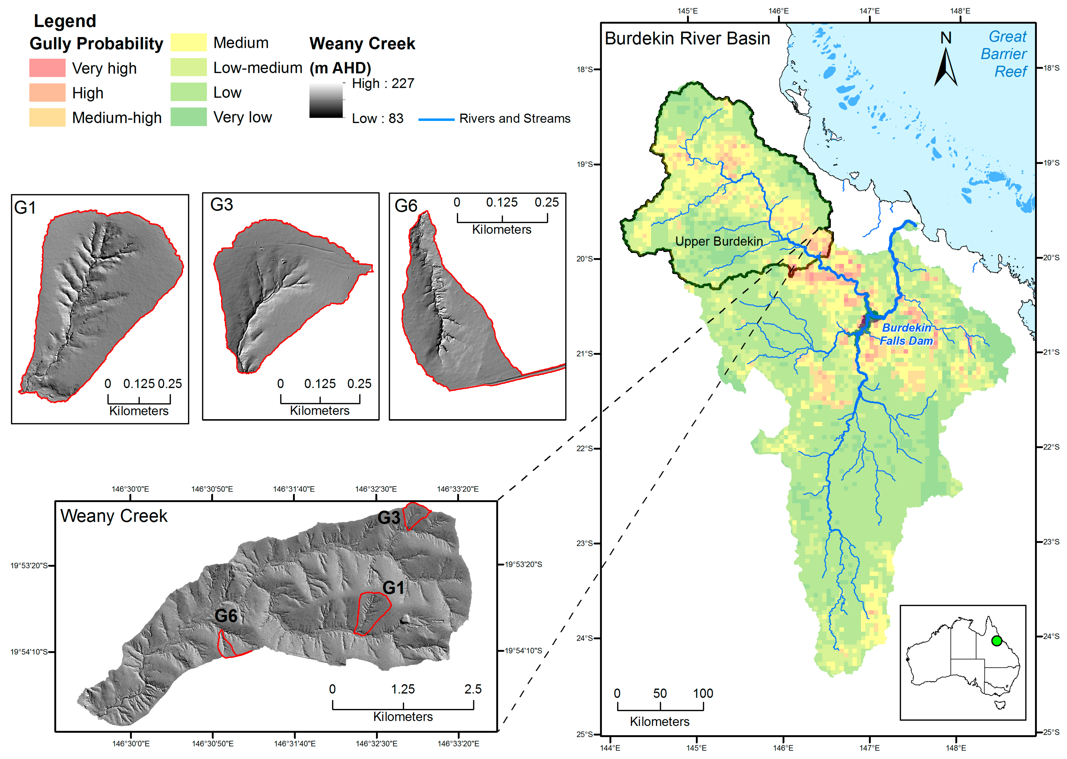
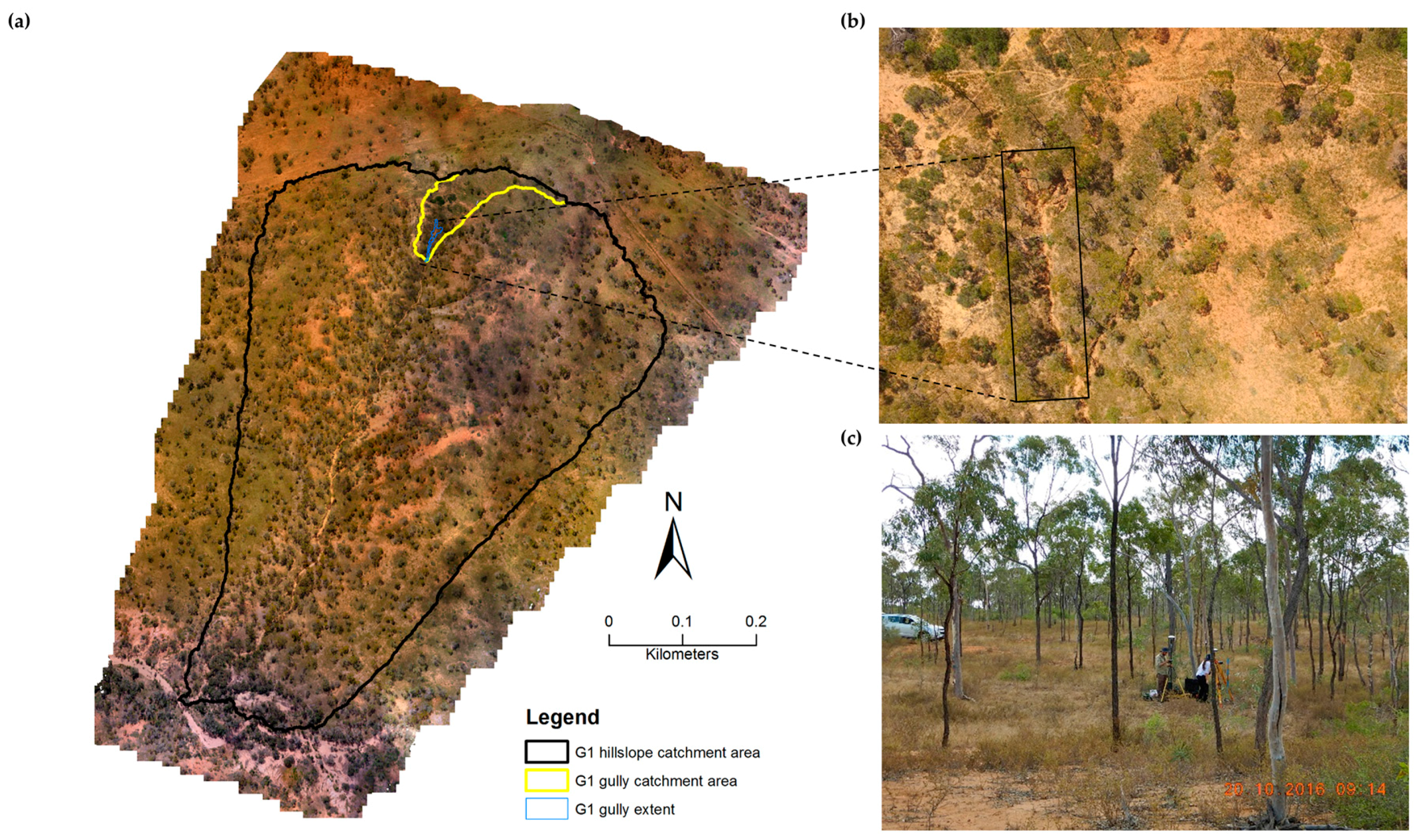
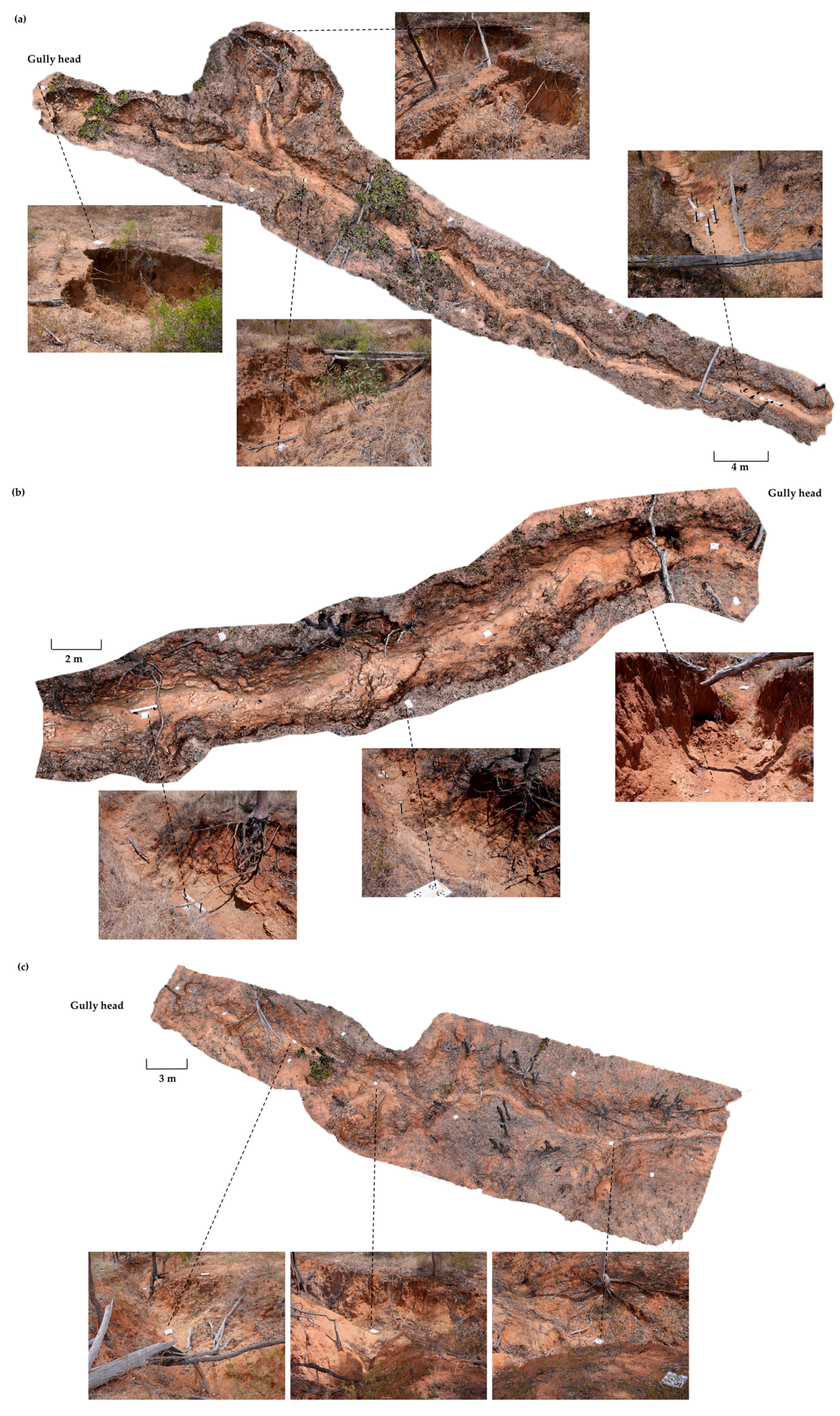
2.1. Study Site
2.2. Datasets
2.2.1. LiDAR
2.2.2. UAV and Ground Survey
2.3. Data Post-Processing
2.3.1. SfM-MVS Workflow, 3D Model, and Ortho-Photo Mosaic Generation
2.3.2. Digital Surface Model (DSM) Generation
2.3.3. Conversion to the Australian Height Datum
2.3.4. Elevation Accuracy of SfM-MVS Topographic Models
3. Results
3.1. Georeferencing Error of Ground Control Points
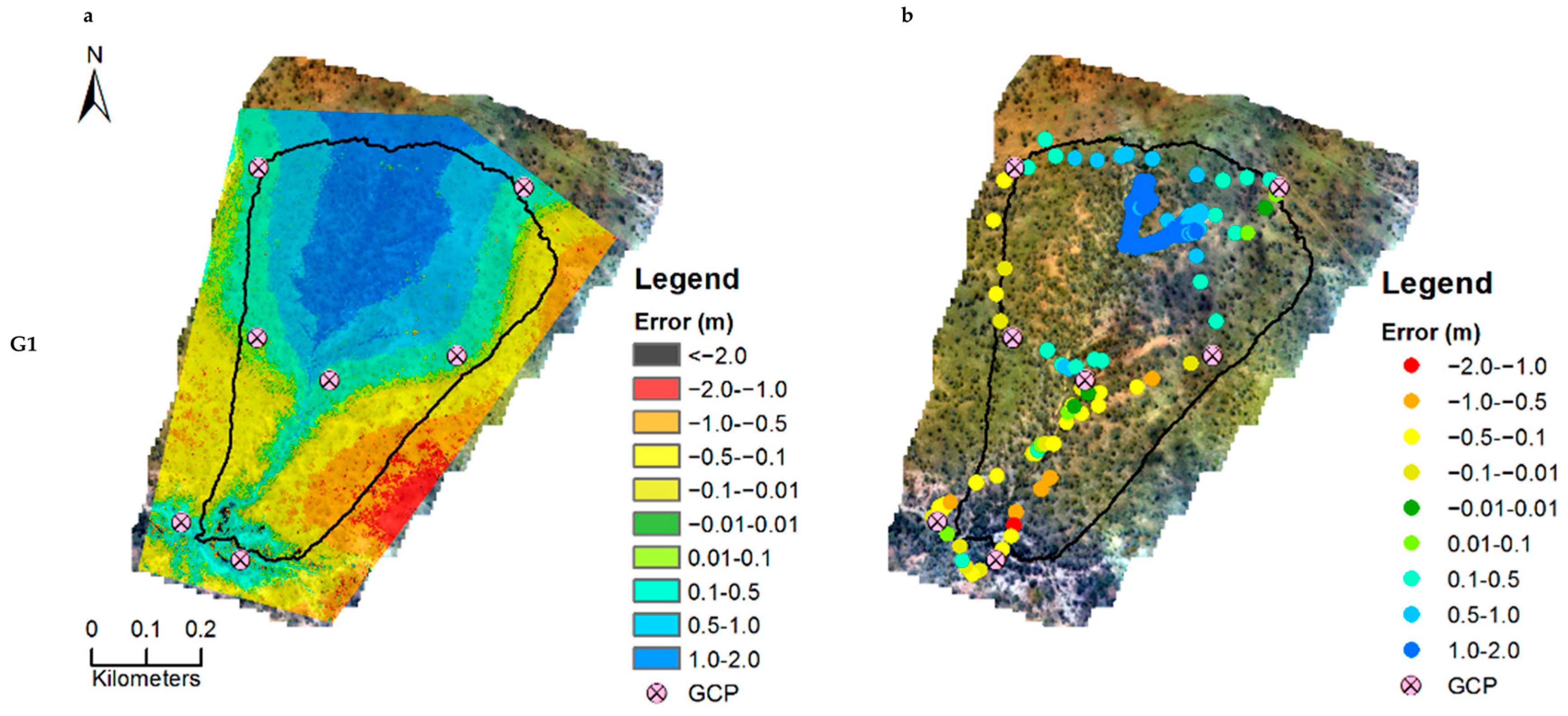
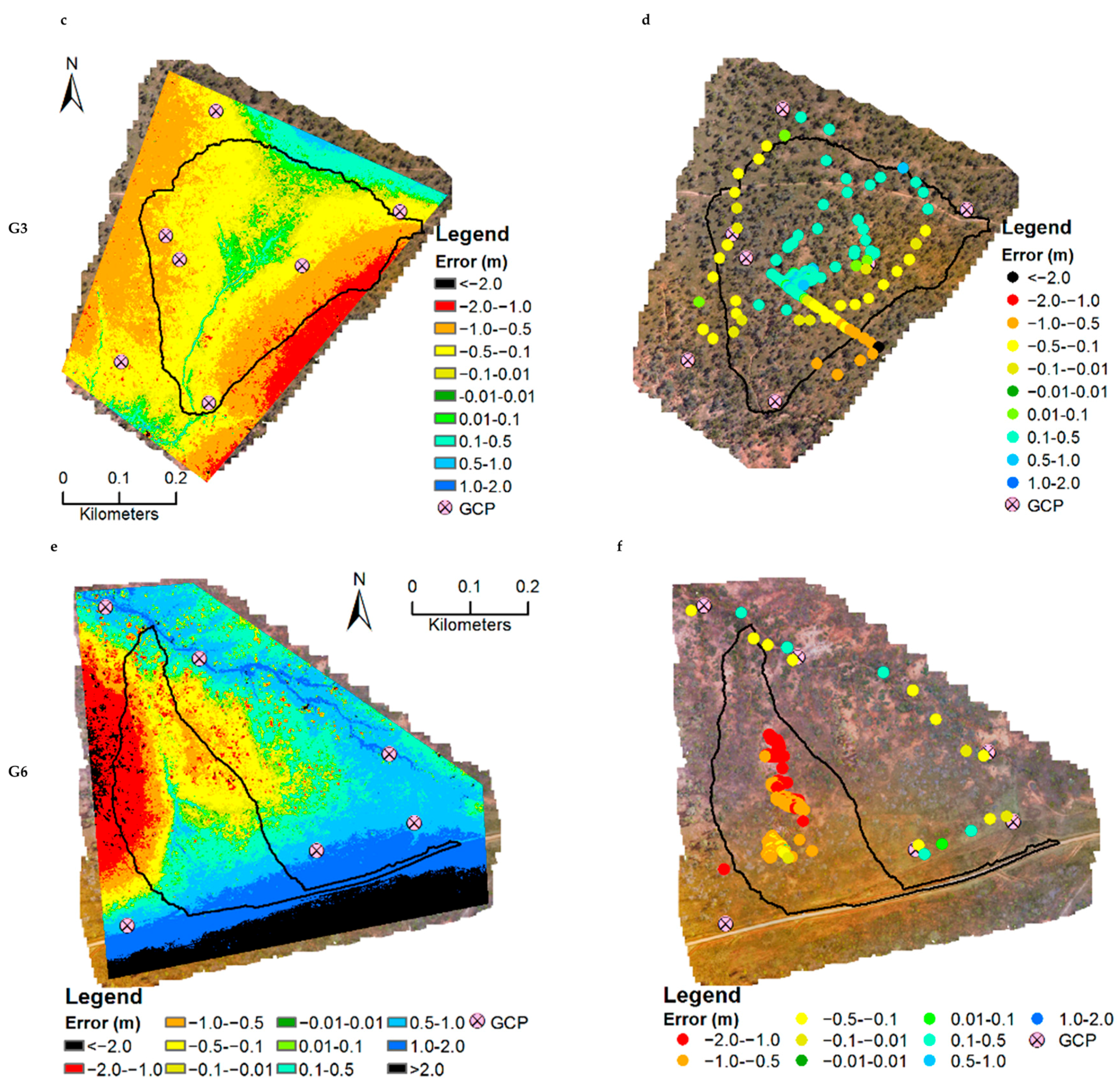
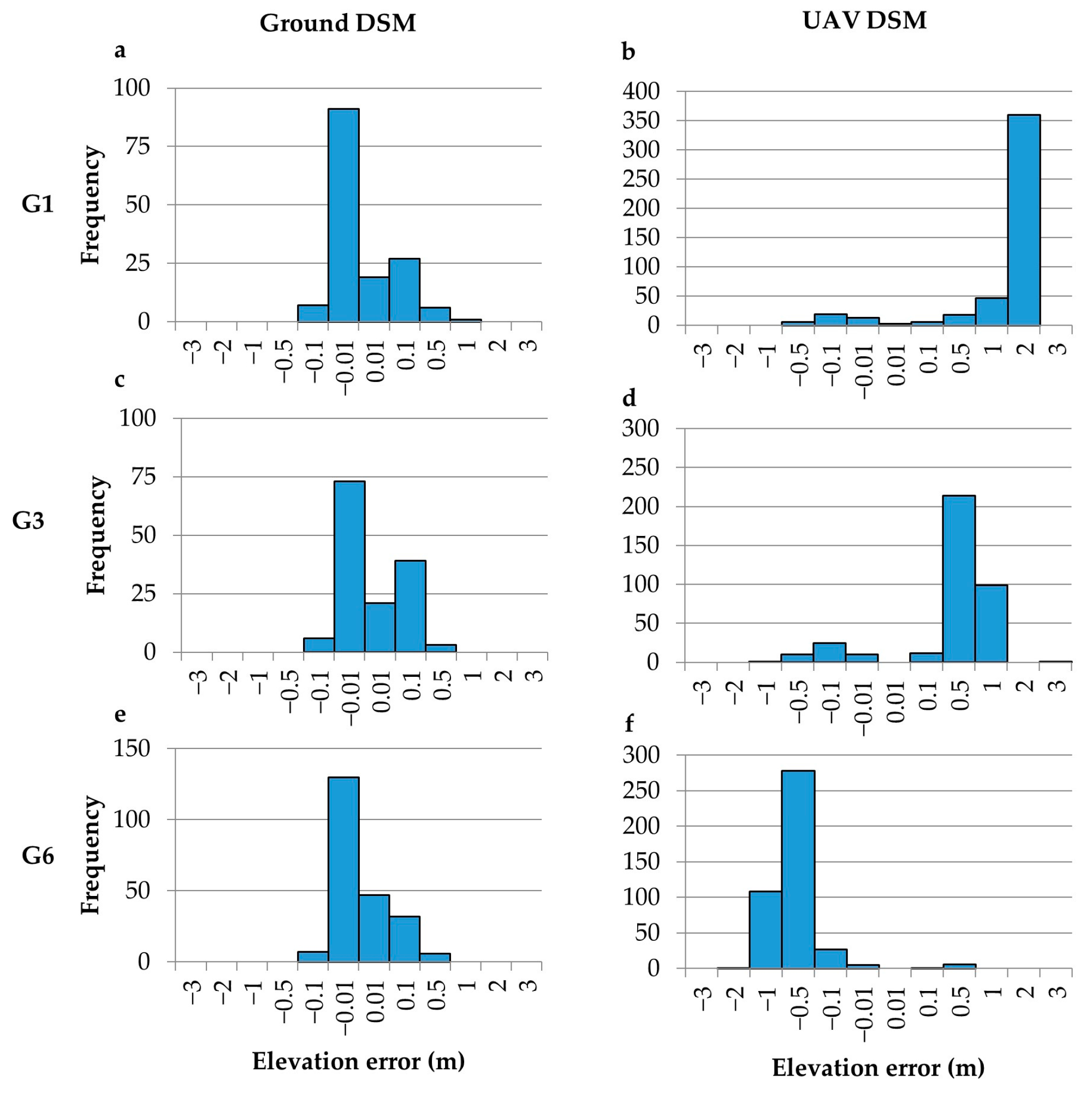
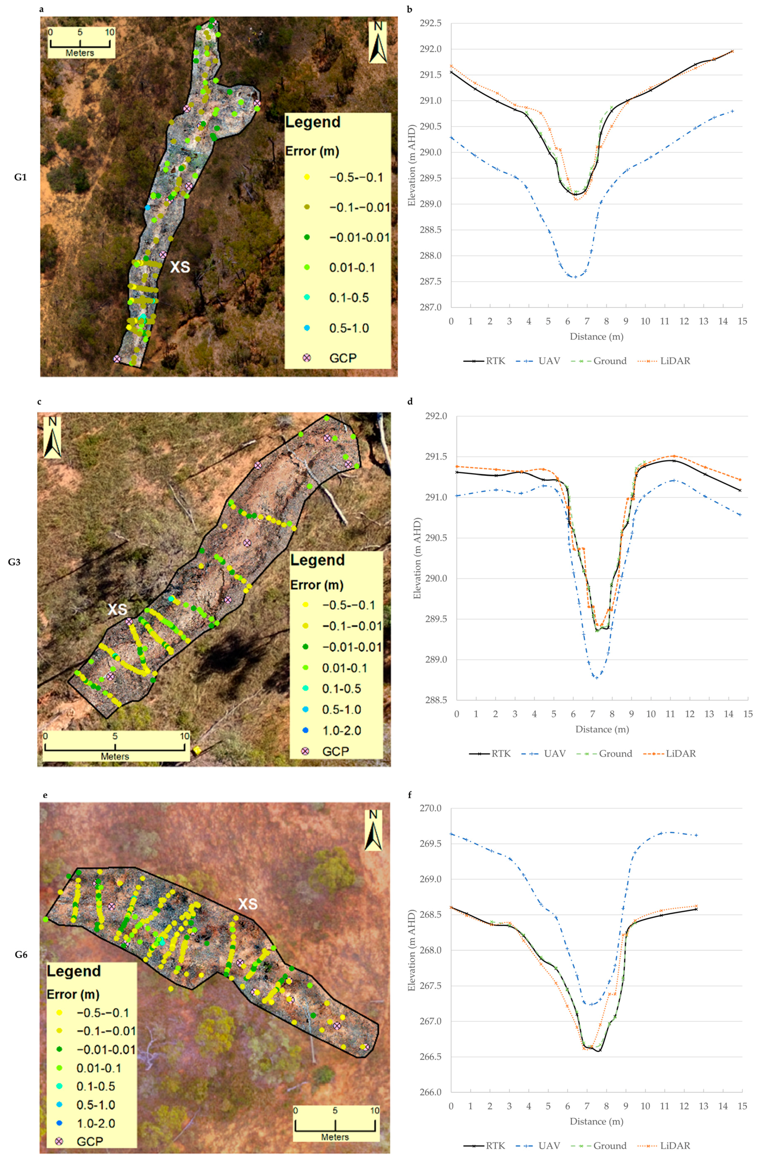
3.2. DSM Elevation Error
3.3. Comparison of Time and Resource Requirements
4. Discussion
4.1. Strengths
4.1.1. Resolution and Accuracy
4.1.2. Low Survey Instrument Costs and Survey Time
4.1.3. High-Resolution Ortho-Photo Mosaics and 3D Models
4.2. Limitations
4.2.1. Vegetation
4.2.2. Methodological Uncertainty
4.2.3. Computational Demands
5. Conclusions
Supplementary Materials
Acknowledgments
Author Contributions
Conflicts of Interest
References
- Poesen, J.; Nachtergaele, J.; Verstraeten, G.; Valentin, C. Gully erosion and environmental change: Importance and research needs. CATENA 2003, 50, 91–133. [Google Scholar] [CrossRef]
- Valentin, C.; Poesen, J.; Li, Y. Gully erosion: Impacts, factors and control. CATENA 2005, 63, 132–153. [Google Scholar] [CrossRef]
- Castillo, C.; Gómez, J.A. A century of gully erosion research: Urgency, complexity and study approaches. Earth-Sci. Rev. 2016, 160, 300–319. [Google Scholar] [CrossRef]
- Poesen, J.; Vanwalleghem, T.; de Vente, J.; Knapen, A.; Verstraeten, G.; Martínez-Casasnovas, J.A. Gully erosion in europe. In Soil Erosion in Europe; Wiley: West Sussex, UK, 2006; pp. 515–536. [Google Scholar]
- Olley, J.M.; Wasson, R.J. Changes in the flux of sediment in the upper murrumbidgee catchment, southeastern Australia, since European settlement. Hydrol. Process. 2003, 17, 3307–3320. [Google Scholar] [CrossRef]
- Wilson, G.V.; Cullum, R.F.; Römkens, M.J.M. Ephemeral gully erosion by preferential flow through a discontinuous soil-pipe. CATENA 2008, 73, 98–106. [Google Scholar] [CrossRef]
- Zhao, J.; Vanmaercke, M.; Chen, L.; Govers, G. Vegetation cover and topography rather than human disturbance control gully density and sediment production on the chinese loess plateau. Geomorphology 2016, 274, 92–105. [Google Scholar] [CrossRef]
- Betts, H.D.; Trustrum, N.A.; Rose, R.C.D. Geomorphic changes in a complex gully system measured from sequential digital elevation models, and implications for management. Earth Surf. Process. Landf. 2003, 28, 1043–1058. [Google Scholar] [CrossRef]
- Lal, R. Restoring land degraded by gully erosion in the tropics. In Advances in Soil Science: Soil Restoration; Lal, R., Stewart, B.A., Cronk, J.K., Eds.; Springer: New York, NY, USA; Berlin, Germany, 1992; Volume 17, pp. 123–152. [Google Scholar]
- Vanmaercke, M.; Poesen, J.; Van Mele, B.; Demuzere, M.; Bruynseels, A.; Golosov, V.; Bezerra, J.F.R.; Bolysov, S.; Dvinskih, A.; Frankl, A.; et al. How fast do gully headcuts retreat? Earth Sci. Rev. 2016, 154, 336–355. [Google Scholar] [CrossRef]
- Liu, X. Airborne lidar for dem generation: Some critical issues. Prog. Phys. Geogr. 2008, 32, 31–49. [Google Scholar] [CrossRef]
- Telling, J.; Lyda, A.; Hartzell, P.; Glennie, C. Review of earth science research using terrestrial laser scanning. Earth Sci. Rev. 2017, 169, 35–68. [Google Scholar] [CrossRef]
- Smith, M.W.; Carrivick, J.L.; Quincey, D.J. Structure from motion photogrammetry in physical geography. Prog. Phys. Geogr. 2015, 1–29. [Google Scholar] [CrossRef]
- Perroy, R.L.; Bookhagen, B.; Asner, G.P.; Chadwick, O.A. Comparison of gully erosion estimates using airborne and ground-based lidar on santa cruz island, california. Geomorphology 2010, 118, 288–300. [Google Scholar] [CrossRef]
- Goodwin, N.R.; Armston, J.; Stiller, I.; Muir, J. Assessing the repeatability of terrestrial laser scanning for monitoring gully topography: A case study from Aratula, Queensland, Australia. Geomorphology 2016, 262, 24–36. [Google Scholar] [CrossRef]
- Westoby, M.J.; Brasington, J.; Glasser, N.F.; Hambrey, M.J.; Reynolds, J.M. ‘Structure-from-motion’ photogrammetry: A low-cost, effective tool for geoscience applications. Geomorphology 2012, 179, 300–314. [Google Scholar] [CrossRef] [Green Version]
- James, M.R.; Robson, S. Straightforward reconstruction of 3d surfaces and topography with a camera: Accuracy and geoscience application. J. Geophys. Res. Earth Surf. 2012, 117, F03017. [Google Scholar] [CrossRef]
- Smith, M.W.; Vericat, D. From experimental plots to experimental landscapes: Topography, erosion and deposition in sub-humid badlands from structure-from-motion photogrammetry. Earth Surf. Process. Landf. 2015, 40, 1656–1671. [Google Scholar] [CrossRef]
- Eltner, A.; Kaiser, A.; Castillo, C.; Rock, G.; Neugirg, F.; Abellán, A. Image-based surface reconstruction in geomorphometry—Merits, limits and developments. Earth Surf. Dyn. 2016, 4, 359–389. [Google Scholar] [CrossRef]
- Piermattei, L.; Carturan, L.; Guarnieri, A. Use of terrestrial photogrammetry based on structure-from-motion for mass balance estimation of a small glacier in the italian alps. Earth Surf. Process. Landf. 2015, 40, 1791–1802. [Google Scholar] [CrossRef]
- Gómez-Gutiérrez, Á.; de Sanjosé-Blasco, J.; de Matías-Bejarano, J.; Berenguer-Sempere, F. Comparing two photo-reconstruction methods to produce high density point clouds and dems in the corral del veleta rock glacier (Sierra Nevada, Spain). Remote Sens. 2014, 6, 5407–5427. [Google Scholar] [CrossRef]
- Stumpf, A.; Malet, J.P.; Allemand, P.; Pierrot-Deseilligny, M.; Skupinski, G. Ground-based multi-view photogrammetry for the monitoring of landslide deformation and erosion. Geomorphology 2015, 231, 130–145. [Google Scholar] [CrossRef]
- Lucieer, A.; de Jong, S.; Turner, D. Mapping landslide displacements using structure from motion (sfm) and image correlation of multi-temporal uav photography. Prog. Phys. Geogr. 2013, 97–116. [Google Scholar] [CrossRef]
- James, M.R.; Varley, N. Identification of structural controls in an active lava dome with high resolution dems: Volcán de Colima, Mexico. Geophys. Res. Lett. 2012, 39, L22303. [Google Scholar] [CrossRef]
- Bemis, S.P.; Micklethwaite, S.; Turner, D.; James, M.R.; Akciz, S.; Thiele, S.T.; Bangash, H.A. Ground-based and uav-based photogrammetry: A multi-scale, high-resolution mapping tool for structural geology and paleoseismology. J. Struct. Geol. 2014, 69, 163–178. [Google Scholar] [CrossRef]
- Javernick, L.; Brasington, J.; Caruso, B. Modeling the topography of shallow braided rivers using structure-from-motion photogrammetry. Geomorphology 2014, 213, 166–182. [Google Scholar] [CrossRef]
- Dietrich, J.T. Riverscape mapping with helicopter-based structure-from-motion photogrammetry. Geomorphology 2016, 252, 144–157. [Google Scholar] [CrossRef]
- Woodget, A.S.; Carbonneau, P.E.; Visser, F.; Maddock, I.P. Quantifying submerged fluvial topography using hyperspatial resolution uas imagery and structure from motion photogrammetry. Earth Surf. Process. Landf. 2015, 40, 47–64. [Google Scholar] [CrossRef]
- Smith, M.W.; Carrivick, J.L.; Hooke, J.; Kirkby, M.J. Reconstructing flash flood magnitudes using ‘structure-from-motion’: A rapid assessment tool. J. Hydrol. 2014, 519, 1914–1927. [Google Scholar] [CrossRef]
- Mancini, F.; Dubbini, M.; Gattelli, M.; Stecchi, F.; Fabbri, S.; Gabbianelli, G. Using unmanned aerial vehicles (uav) for high-resolution reconstruction of topography: The structure from motion approach on coastal environments. Remote Sens. 2013, 5, 6880. [Google Scholar] [CrossRef] [Green Version]
- Bryson, M.; Johnson-Roberson, M.; Murphy, R.J.; Bongiorno, D. Kite aerial photography for low-cost, ultra-high spatial resolution multi-spectral mapping of intertidal landscapes. PLoS ONE 2013, 8, e73550. [Google Scholar] [CrossRef] [PubMed]
- Figueira, W.; Ferrari, R.; Weatherby, E.; Porter, A.; Hawes, S.; Byrne, M. Accuracy and precision of habitat structural complexity metrics derived from underwater photogrammetry. Remote Sens. 2015, 7, 15859–16900. [Google Scholar] [CrossRef]
- Leon, J.X.; Roelfsema, C.M.; Saunders, M.I.; Phinn, S.R. Measuring coral reef terrain roughness using ‘structure-from-motion’ close-range photogrammetry. Geomorphology 2015, 242, 21–28. [Google Scholar] [CrossRef]
- Brunier, G.; Fleury, J.; Anthony, E.J.; Gardel, A.; Dussouillez, P. Close-range airborne structure-from-motion photogrammetry for high-resolution beach morphometric surveys: Examples from an embayed rotating beach. Geomorphology 2016, 261, 76–88. [Google Scholar] [CrossRef]
- Nouwakpo, S.K.; Weltz, M.A.; McGwire, K. Assessing the performance of structure-from-motion photogrammetry and terrestrial lidar for reconstructing soil surface microtopography of naturally vegetated plots. Earth Surf. Process. Landf. 2016, 41, 308–322. [Google Scholar] [CrossRef]
- Ouédraogo, M.M.; Degré, A.; Debouche, C.; Lisein, J. The evaluation of unmanned aerial system-based photogrammetry and terrestrial laser scanning to generate dems of agricultural watersheds. Geomorphology 2014, 214, 339–355. [Google Scholar] [CrossRef]
- Nouwakpo, S.K.; James, M.R.; Weltz, M.A.; Huang, C.H.; Chagas, I.; Lima, L. Evaluation of structure from motion for soil microtopography measurement. Photogramm. Rec. 2014, 29, 297–316. [Google Scholar] [CrossRef]
- Castillo, C.; James, M.; Redel-Macías, M.; Pérez, R.; Gómez, J. Sf3m software: 3-d photo-reconstruction for non-expert users and its application to a gully network. Soil 2015, 1, 583–594. [Google Scholar] [CrossRef]
- Castillo, C.; Taguas, E.V.; Zarco-Tejada, P.; James, M.R.; Gómez, J.A. The normalized topographic method: An automated procedure for gully mapping using gis. Earth Surf. Process. Landf. 2014, 39, 2002–2015. [Google Scholar] [CrossRef]
- Gómez-Gutiérrez, Á.; Schnabel, S.; Berenguer-Sempere, F.; Lavado-Contador, F.; Rubio-Delgado, J. Using 3d photo-reconstruction methods to estimate gully headcut erosion. CATENA 2014, 120, 91–101. [Google Scholar] [CrossRef]
- Stöcker, C.; Eltner, A.; Karrasch, P. Measuring gullies by synergetic application of uav and close range photogrammetry—A case study from andalusia, spain. CATENA 2015, 132, 1–11. [Google Scholar] [CrossRef]
- Di Stefano, C.; Ferro, V.; Palmeri, V.; Pampalone, V.; Agnello, F. Testing the use of an image-based technique to measure gully erosion at sparacia experimental area. Hydrol. Process. 2017, 31, 573–585. [Google Scholar] [CrossRef]
- D’Oleire-Oltmanns, S.; Marzolff, I.; Peter, K.; Ries, J. Unmanned Aerial Vehicle (UAV) for monitoring soil erosion in morocco. Remote Sens. 2012, 4, 3390. [Google Scholar] [CrossRef]
- James, M.R.; Robson, S.; d’Oleire-Oltmanns, S.; Niethammer, U. Optimising uav topographic surveys processed with structure-from-motion: Ground control quality, quantity and bundle adjustment. Geomorphology 2017, 280, 51–66. [Google Scholar] [CrossRef]
- Peter, K.D.; d’Oleire-Oltmanns, S.; Ries, J.B.; Marzolff, I.; Ait Hssaine, A. Soil erosion in gully catchments affected by land-levelling measures in the souss basin, morocco, analysed by rainfall simulation and uav remote sensing data. CATENA 2014, 113, 24–40. [Google Scholar] [CrossRef]
- Frankl, A.; Stal, C.; Abraha, A.; Nyssen, J.; Rieke-Zapp, D.; De Wulf, A.; Poesen, J. Detailed recording of gully morphology in 3D through image-based modelling. CATENA 2015, 127, 92–101. [Google Scholar] [CrossRef] [Green Version]
- Glendell, M.; McShane, G.; Farrow, L.; James, M.R.; Quinton, J.; Anderson, K.; Evans, M.; Benaud, P.; Rawlins, B.; Morgan, D.; et al. Testing the utility of structure-from-motion photogrammetry reconstructions using small unmanned aerial vehicles and ground photography to estimate the extent of upland soil erosion. Earth Surf. Process. Landf. 2017. [Google Scholar] [CrossRef]
- Christian, P.; Davis, J. Hillslope gully photogeomorphology using structure-from-motion. Z. Geomorphol. Suppl. Issues 2016, 60, 59–78. [Google Scholar] [CrossRef]
- Gesch, K.R.; Wells, R.R.; Cruse, R.M.; Momm, H.G.; Dabney, S.M. Quantifying uncertainty of measuring gully morphological evolution with close-range digital photogrammetry. Soil Sci. Soc. Am. J. 2015, 79, 650–659. [Google Scholar] [CrossRef]
- Wells, R.R.; Momm, H.G.; Castillo, C. Quantifying uncertainty in high-resolution remotely sensed topographic surveys for ephemeral gully channel monitoring. Earth Surf. Dyn. 2017, 5, 347–367. [Google Scholar] [CrossRef]
- Lannoeye, W.; Stal, C.; Guyassa, E.; Zenebe, A.; Nyssen, J.; Frankl, A. The use of sfm-photogrammetry to quantify and understand gully degradation at the temporal scale of rainfall events: An example from the ethiopian drylands. Phys. Geogr. 2016, 37, 430–451. [Google Scholar] [CrossRef]
- Liu, K.; Ding, H.; Tang, G.; Na, J.; Huang, X.; Xue, Z.; Yang, X.; Li, F. Detection of catchment-scale gully-affected areas using unmanned Aerial Vehicle (UAV) on the chinese loess plateau. ISPRS Int. J. Geo-Inf. 2016, 5, 238. [Google Scholar] [CrossRef]
- Wang, R.; Zhang, S.; Pu, L.; Yang, J.; Yang, C.; Chen, J.; Guan, C.; Wang, Q.; Chen, D.; Fu, B.; et al. Gully erosion mapping and monitoring at multiple scales based on multi-source remote sensing data of the sancha river catchment, northeast china. ISPRS Int. J. Geo-Inf. 2016, 5, 200. [Google Scholar] [CrossRef]
- Zhang, B.; Xiong, D.; Su, Z.; Yang, D.; Dong, Y.; Xiao, L.; Zhang, S.; Shi, L. Effects of initial step height on the headcut erosion of bank gullies: A case study using a 3d photo-reconstruction method in the dry-hot valley region of southwest china. Phys. Geogr. 2016, 37, 409–429. [Google Scholar] [CrossRef]
- Meadows, M.E.; Thomas, D.S.G. Tropical savannas. In Geomorphology and Global Environmental Change; Slaymaker, O., Spencer, T., Embleton-Hamann, C., Eds.; Cambridge University Press: Cambridge, UK, 2009; pp. 248–275. [Google Scholar]
- Brooks, A.; Spencer, J.; Knight, J. Alluvial gully erosion: An example from the mitchell fluvial megafan, Queensland, Australia. Earth Surf. Process. Landf. 2009, 34, 43–48. [Google Scholar] [CrossRef]
- Bartley, R.; Hawdon, A.; Post, D.A.; Roth, C.H. A sediment budget for a grazed semi-arid catchment in the Burdekin Basin, Australia. Geomorphology 2007, 87, 302–321. [Google Scholar] [CrossRef]
- Bartley, R.; Bainbridge, Z.T.; Lewis, S.E.; Kroon, F.J.; Wilkinson, S.N.; Brodie, J.E.; Silburn, D.M. Relating sediment impacts on coral reefs to watershed sources, processes and management: A review. Sci. Total Environ. 2014, 468–469, 1138–1153. [Google Scholar] [CrossRef] [PubMed]
- Brodie, J.; Waterhouse, J.; Schaffelke, B.; Kroon, F.; Thorburn, P.; Rolfe, J.; Johnson, J.; Fabricius, K.; Lewis, S.; Devlin, M.; et al. 2013 Scientific Consensus Statement: Land Use Impacts on Great Barrier Reef Water Quality and Ecosystem Condition; The State of Queensland: Brisbane, Australia, 2013.
- Kroon, F.J.; Thorburn, P.; Schaffelke, B.; Whitten, S. Towards protecting the Great Barrier Reef from land-based pollution. Glob. Chang. Biol. 2016, 22, 1985–2002. [Google Scholar] [CrossRef] [PubMed]
- Thorburn, P.J.; Wilkinson, S.N. Conceptual frameworks for estimating the water quality benefits of improved agricultural management practices in large catchments. Agric. Ecosyst. Environ. 2013, 180, 192–209. [Google Scholar] [CrossRef]
- Waters, D.; Carroll, C.; Ellis, R.; Hateley, L.; McCloskey, G.; Packett, R.; Dougall, C.; Fentie. Modelling Reductions of Pollutant Loads Due to Improved Management Practices in the Great Barrier Reef Catchments—Whole of Gbr; Queensland Department of Natural Resources and Mines: Toowoomba, Australia, 2014.
- Caitcheon, G.G.; Olley, J.M.; Pantus, F.; Hancock, G.; Leslie, C. The dominant erosion processes supplying fine sediment to three major rivers in tropical Australia, the Daly (nt), Mitchell (qld) and Flinders (qld) rivers. Geomorphology 2012, 151–152, 188–195. [Google Scholar] [CrossRef]
- Hughes, A.O.; Olley, J.M.; Croke, J.C.; McKergow, L.A. Sediment source changes over the last 250 years in a dry-tropical catchment, central Queensland, Australia. Geomorphology 2009, 104, 262–275. [Google Scholar] [CrossRef]
- Tims, S.G.; Everett, S.E.; Fifield, L.K.; Hancock, G.J.; Bartley, R. Plutonium as a tracer of soil and sediment movement in the herbert river, Australia. Nucl. Instrum. Methods Phys. Res. B 2010, 268, 1150–1154. [Google Scholar] [CrossRef]
- Wasson, R.J.; Furlonger, L.; Parry, D.; Pietsch, T.; Valentine, E.; Williams, D. Sediment sources and channel dynamics, daly river, northern Australia. Geomorphology 2010, 114, 161–174. [Google Scholar] [CrossRef]
- Olley, J.; Brooks, A.; Spencer, J.; Pietsch, T.; Borombovits, D. Subsoil erosion dominates the supply of fine sediment to rivers draining into princess charlotte bay, Australia. J. Environ. Radioact. 2013, 124, 121–129. [Google Scholar] [CrossRef] [PubMed]
- Furuichi, T.; Olley, J.; Wilkinson, S.; Lewis, S.; Bainbridge, Z.; Burton, J. Paired geochemical tracing and load monitoring analysis for identifying sediment sources in a large catchment draining into the Great Barrier Reef Lagoon. Geomorphology 2016, 266, 41–52. [Google Scholar] [CrossRef]
- Fabricius, K.E. Effects of terrestrial runoff on the ecology of corals and coral reefs: Review and synthesis. Mar. Pollut. Bull. 2005, 50, 125–146. [Google Scholar] [CrossRef] [PubMed]
- Brodie, J.E.; Lewis, S.E.; Collier, C.J.; Wooldridge, S.; Bainbridge, Z.T.; Waterhouse, J.; Rasheed, M.A.; Honchin, C.; Holmes, G.; Fabricius, K. Setting ecologically relevant targets for river pollutant loads to meet marine water quality requirements for the Great Barrier Reef, Australia: A preliminary methodology and analysis. Ocean Coast. Manag. 2017, 143, 136–147. [Google Scholar] [CrossRef]
- Wilkinson, S.N.; Bartley, R.; Hairsine, P.B.; Bui, E.N.; Gregory, L.; Henderson, A.E. Managing Gully Erosion as an Efficient Approach to Improving Water Quality in the Great Barrier Reef Lagoon; Report to the Department of the Environment; CSIRO Land and Water: Canberra, Australia, 2015. [Google Scholar]
- Hughes, A.; Prosser, P.; Stevenson, J.; Scott, A.; Lu, H.; Gallant, J.; Moran, C. Gully Erosion Mapping for the National Land and Water Audit; Technical Report 26/01; CSIRO Land and Water: Canberra, Australia, 2001. [Google Scholar]
- Kuhnert, P.; Kinsey-Henderson, A.; Bartley, R.; Herr, A. Incorporating uncertainty in gully erosion calculations using the random forests modelling approach. Environmetrics 2010, 21, 493–509. [Google Scholar] [CrossRef]
- McKergow, L.A.; Prosser, I.P.; Hughes, A.O.; Brodie, J. Sources of sediment to the great barrier reef world heritage area. Mar. Pollut. Bull. 2005, 51, 200–211. [Google Scholar] [CrossRef] [PubMed]
- Waters, D.; Carroll, C.; Ellis, R.; McCloskey, G.; Hateley, L.; Packett, B.; Dougasll, C.; Fentie, B. Catchment modelling scenarios to inform gbr water quality targets. In Proceedings of the 20th International Congress on Modelling and Simulation, Adelaide, Australia, 1–6 December 2013. [Google Scholar]
- Tindall, D.; Marchand, B.; Gilad, U.; Goodwin, N.; Denham, R.; Byer, S. Gully Mapping and Drivers in the Grazing Lands of the Burdekin Catchment; Rp66g Synthesis Report; The State of Queensland (Department of Science, Information Technology, Innovation and the Arts): Brisbane, Australia, 2014.
- Wilkinson, S.N.; Dougall, C.; Kinsey-Henderson, A.E.; Searle, R.; Ellis, R.; Bartley, R. Development of a time-stepping sediment budget model for assessing land use impacts in large river basins. Sci. Total Environ. 2014, 468–469, 1210–1224. [Google Scholar] [CrossRef] [PubMed]
- Goodwin, N.R.; Armston, J.D.; Muir, J.; Stiller, I. Monitoring gully change: A comparison of airborne and terrestrial laser scanning using a case study from Aratula, Queensland. Geomorphology 2017, 282, 195–208. [Google Scholar] [CrossRef]
- Shellberg, J.G.; Brooks, A.P.; Spencer, J.; Ward, D. The hydrogeomorphic influences on alluvial gully erosion along the Mitchell River fluvial megafan. Hydrol. Process. 2013, 27, 1086–1104. [Google Scholar] [CrossRef]
- Hancock, G.R.; Evans, K.G. Gully position, characteristics and geomorphic thresholds in an undisturbed catchment in northern Australia. Hydrol. Process. 2006, 20, 2935–2951. [Google Scholar] [CrossRef]
- Bartley, R.; Croke, J.; Bainbridge, Z.T.; Austin, J.M.; Kuhnert, P.M. Combining contemporary and long-term erosion rates to target erosion hot-spots in the Great Barrier Reef, Australia. Anthropocene 2015, 10, 1–12. [Google Scholar] [CrossRef]
- Isbell, R.F. The Australian Soil Classification; CSIRO Publishing: Collingwood, Australia, 1996. [Google Scholar]
- Bartley, R.; Corfield, J.P.; Abbott, B.N.; Hawdon, A.A.; Wilkinson, S.N.; Nelson, B. Impacts of improved grazing land management on sediment yields, part 1: Hillslope processes. J. Hydrol. 2010, 389, 237–248. [Google Scholar] [CrossRef]
- Gilad, U.; Denham, R.; Tindall, D. Gullies, google earth and the Great Barrier Reef: A remote sensing methodology for mapping gullies over extensive areas. In Proceedings of the International Archives of the Photogrammetry, Remote Sensing and Spatial Information Science, XXII ISPRS Congress, Melbourne, Australia, 25 August–1 September 2012; Volume XXXIX-B8, pp. 469–473. [Google Scholar]
- Wilkinson, S.N.; Kinsey-Henderson, A.E.; Hawdon, A.A.; Ellis, T.W.; Nicholas, D.M. Gully Erosion and Its Response to Grazing Practices in the Upper Burdekin Catchment. A Report to nq Dry Tropics for the Paddock to Reef Program; CSIRO Water for a Healthy Country Flagship: Canberra, Australia, 2013. [Google Scholar]
- Petheram, C.; McMahon, T.A.; Peel, M.C. Flow characteristics of rivers in northern Australia: Implications for development. J. Hydrol. 2008, 357, 93–111. [Google Scholar] [CrossRef]
- Nicholls, N. The el niño/southern oscillation and Australian vegetation. Vegetatio 1991, 91, 23–36. [Google Scholar] [CrossRef]
- Jarihani, B.; Sidle, R.C.; Bartley, R.; Roth, C.H.; Wilkinson, S.N. Characterisation of hydrological response to rainfall at multi spatio-temporal scales in savannas of semi-arid Australia. Water 2017, 9, 540. [Google Scholar] [CrossRef]
- Mott, J.J.; Williams, J.; Andrew, M.H.; Gillison, A.N. Chapter 7: Australian savanna ecosystems. In Ecology and Management of the World’s Savannas; Tothill, J.C., Mott, J.J., Eds.; Australian Academy of Sciences: Canberra, Australia, 1985; pp. 56–82. [Google Scholar]
- Williams, R.J.; Cook, G.D.; Gill, A.M.; Moore, P.H.R. Fire regime, fire intensity and tree survival in a tropical savanna in northern Australia. Aust. J. Ecol. 1999, 24, 50–59. [Google Scholar] [CrossRef]
- Williams, R.; Gill, A.; Moore, P. Seasonal changes in fire behaviour in a tropical savanna in northern Australia. Int. J. Wildland Fire 1998, 8, 227–239. [Google Scholar] [CrossRef]
- Townsend, S.A.; Douglas, M.M. The effect of three fire regimes on stream water quality, water yield and export coefficients in a tropical savanna (northern Australia). J. Hydrol. 2000, 229, 118–137. [Google Scholar] [CrossRef]
- Wilkinson, S.N.; Kinsey-Henderson, A.E.; Hawdon, A.A.; Hairsine, P.B.; Bartley, R.; Baker, B. Gully erosion processes, dynamics and controls in a tropical savannah. Earth Surf. Process. Landf. 2017. under review. [Google Scholar]
- Sibson, R. A brief description of natural neighbor interpolation. In Interpolating Multivariate Data; Barnett, V., Ed.; John Wiley & Sons: West Sussex, UK, 1981; pp. 21–36. [Google Scholar]
- Dà-Jiāng Innovations Science and Technology Co (DJI). Phantom 3 Professional User Manual v1.8; DJI: Shenzhen, China, 2016. [Google Scholar]
- Maps Made Easy. Maps made easy-home. Available online: https://www.mapsmadeeasy.com/ (accessed on 3 March 2017).
- AgiSoft LLC. Agisoft Photoscan Professional v1.3 User Manual. Available online: http://www.agisoft.com/downloads/user-manuals/ (accessed on 3 March 2017).
- Lowe, D.G. Distinctive image features from scale-invariant keypoints. Int. J. Comput. Vis. 2004, 60, 91–110. [Google Scholar] [CrossRef]
- Girardeau-Montaut, D. Cloudcompare: 3D Point Cloud and Mesh Processing Software, v2.8. Available online: http://www.danielgm.net/cc/ (accessed on 3 March 2017).
- Geoscience Australia. Ausgeoid09. Available online: http://www.ga.gov.au/ausgeoid/nvalcomp.jsp (accessed on 3 March 2017).
- Cook, K.L. An evaluation of the effectiveness of low-cost uavs and structure from motion for geomorphic change detection. Geomorphology 2017, 278, 195–208. [Google Scholar] [CrossRef]
- Carrivick, J.L.; Smith, M.W.; Quincey, D.J. Quality assessment. In Structure from Motion in the Geosciences; John Wiley & Sons, Ltd: West Sussex, UK, 2016; pp. 97–123. [Google Scholar]
- Tonkin, T.N.; Midgley, N.G.; Graham, D.J.; Labadz, J.C. The potential of small unmanned aircraft systems and structure-from-motion for topographic surveys: A test of emerging integrated approaches at cwm idwal, north Wales. Geomorphology 2014, 226, 35–43. [Google Scholar] [CrossRef] [Green Version]
- Kaiser, A.; Neugirg, F.; Rock, G.; Müller, C.; Haas, F.; Ries, J.; Schmidt, J. Small-scale surface reconstruction and volume calculation of soil erosion in complex moroccan gully morphology using structure from motion. Remote Sens. 2014, 6, 7050–7080. [Google Scholar] [CrossRef] [Green Version]
- Castillo, C.; Pérez, R.; James, M.R.; Quinton, J.N.; Taguas, E.V.; Gómez, J.A. Comparing the accuracy of several field methods for measuring gully erosion. Soil Sci. Soc. Am. J. 2012, 76. [Google Scholar] [CrossRef] [Green Version]
- Bartley, R.; Goodwin, N.; Henderson, A.E.; Hawdon, A.; Tindall, D.; Wilkinson, S.N.; Baker, B. A Comparison of Tools for Monitoring and Evaluating Channel Change; Report to the national environmental science programme; Reef and Rainforest Research Centre Limited: Cairns, Australia, 2016. [Google Scholar]
- Civil Aviation Safety Authority. Flying Drones/Remotely Piloted Aircraft in Australia. Available online: https://www.casa.gov.au/aircraft/landing-page/flying-drones-australia (accessed on 7 May 2017).
- Jarihani, A.A.; Callow, J.N.; McVicar, T.R.; Van Niel, T.G.; Larsen, J.R. Satellite-derived digital elevation model (dem) selection, preparation and correction for hydrodynamic modelling in large, low-gradient and data-sparse catchments. J. Hydrol. 2015, 524, 489–506. [Google Scholar] [CrossRef]
- Cunliffe, A.M.; Brazier, R.E.; Anderson, K. Ultra-fine grain landscape-scale quantification of dryland vegetation structure with drone-acquired structure-from-motion photogrammetry. Remote Sens. Environ. 2016, 183, 129–143. [Google Scholar] [CrossRef] [Green Version]
- Brodu, N.; Lague, D. 3D terrestrial lidar data classification of complex natural scenes using a multi-scale dimensionality criterion: Applications in geomorphology. ISPRS J. Photogramm. Remote Sens. 2012, 68, 121–134. [Google Scholar] [CrossRef] [Green Version]
- Jensen, J.; Mathews, A. Assessment of image-based point cloud products to generate a bare earth surface and estimate canopy heights in a woodland ecosystem. Remote Sens. 2016, 8, 50. [Google Scholar] [CrossRef]
- Serifoglu, C.; Gungor, O.; Yilmaz, V. Performance evaluation of different ground filtering algorithms for uav-based point clouds. Int. Arch. Photogramm. Remote Sens. Spat. Inf. Sci. 2016, 41. [Google Scholar] [CrossRef]
- Dandois, J.P.; Ellis, E.C. High spatial resolution three-dimensional mapping of vegetation spectral dynamics using computer vision. Remote Sens. Environ. 2013, 136, 259–276. [Google Scholar] [CrossRef]
- Tonkin, T.; Midgley, N. Ground-control networks for image based surface reconstruction: An investigation of optimum survey designs using uav derived imagery and structure-from-motion photogrammetry. Remote Sens. 2016, 8, 786. [Google Scholar] [CrossRef]
- James, M.R.; Robson, S. Mitigating systematic error in topographic models derived from uav and ground-based image networks. Earth Surf. Process. Landf. 2014, 39, 1413–1420. [Google Scholar] [CrossRef]
- Clapuyt, F.; Vanacker, V.; Van Oost, K. Reproducibility of uav-based earth topography reconstructions based on structure-from-motion algorithms. Geomorphology 2016, 260, 4–15. [Google Scholar] [CrossRef]
- Eltner, A.; Schneider, D. Analysis of different methods for 3D reconstruction of natural surfaces from parallel-axes uav images. Photogramm. Rec. 2015, 30, 279–299. [Google Scholar] [CrossRef]
- Nex, F.; Remondino, F. Uav for 3D mapping applications: A review. Appl. Geomat. 2014, 6, 1–15. [Google Scholar] [CrossRef]
- Vautherin, J.; Rutishauser, S.; Schneider-Zapp, K.; Choi, H.F.; Chovancova, V.; Glass, A.; Strecha, C. Photogrammetric accuracy and modeling of rolling shutter cameras. ISPRS Ann. Photogramm. Remote Sens. Spat. Inf. Sci. 2016, 3, 139–146. [Google Scholar] [CrossRef]


| Survey | Camera Name | Sensor | Sensor Resolution | Lens | Image Resolution | Mode |
|---|---|---|---|---|---|---|
| UAV | DJI FC300X | 1/2.3″ CMOS | 12.4 MP | DJI 20 mm (35 mm format equivalent) f/2.8 | 12 MP | Automatic (no flash) |
| Ground | Panasonic GH3 | 4/3″ CMOS | 16.1 MP | Panasonic Lumix G 20 mm f/1.7 II ASPH prime | 8 MP | Automatic (no flash) |
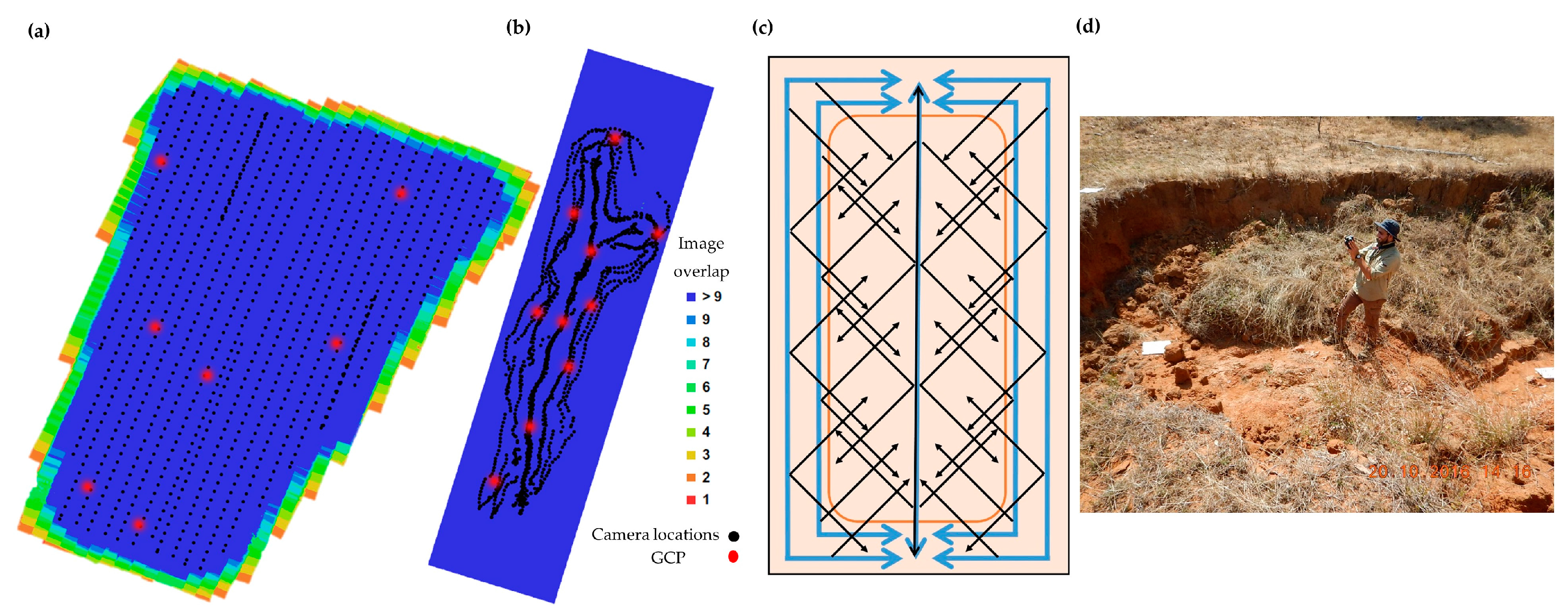
| System | Survey | ~Altitude of Image Capture (m) | Forward Overlap (%) | Side Overlap (%) | Number of Images Captured | Image Overlap (Num. of Images) | Area Covered (m2) | Ground Sampling Distance (cm pix−1) | Number of GCPs | Number of Validation Points |
|---|---|---|---|---|---|---|---|---|---|---|
| G1 | UAV | 99 | 80 | 75 | 938 | >9 | 715,000 | 3.31 | 7 | 151 |
| Ground | 1.5 | - | - | 1747 | >9 | 650 | 0.129 | 10 | 471 | |
| G3 | UAV | 86 | 80 | 75 | 451 | >9 | 412,000 | 2.89 | 7 | 142 |
| Ground | 1.5 | - | - | 935 | >9 | 350 | 0.129 | 7 | 372 | |
| G6 | UAV | 97 | 80 | 75 | 603 | >9 | 451,000 | 3.05 | 6 | 222 |
| Ground | 1.5 | - | - | 1228 | >9 | 750 | 0.132 | 10 | 426 |
| Coordinate Error | G1 | G3 | G6 | |||
|---|---|---|---|---|---|---|
| UAV | Ground | UAV | Ground | UAV | Ground | |
| X (m) | 0.007 | 0.011 | 0.002 | 0.008 | 0.006 | 0.006 |
| Y (m) | 0.009 | 0.006 | 0.002 | 0.007 | 0.008 | 0.010 |
| Z (m) | 0.025 | 0.018 | 0.013 | 0.012 | 0.003 | 0.010 |
| Total error (m) | 0.027 | 0.022 | 0.013 | 0.016 | 0.010 | 0.015 |
| Total error (pixels) | 0.350 | 0.140 | 0.279 | 3.351 | 0.270 | 0.239 |
| System | Scale | RMSE (m) | MAE (m) | ME (m) | |||
|---|---|---|---|---|---|---|---|
| UAV DSM | Ground DSM | UAV DSM | Ground DSM | UAV DSM | Ground DSM | ||
| G1 | Gully | 1.538 | 0.092 | 1.527 | 0.052 | 1.527 | −0.014 |
| Hillslope | 1.307 | NA | 1.220 | NA | 1.180 | NA | |
| G3 | Gully | 0.519 | 0.074 | 0.492 | 0.046 | 0.485 | −0.013 |
| Hillslope | 0.461 | NA | 0.406 | NA | 0.326 | NA | |
| G6 | Gully | 0.838 | 0.057 | 0.813 | 0.038 | −0.813 | −0.015 |
| Hillslope | 0.903 | NA | 0.851 | NA | −0.844 | NA | |
| System | Scale | RMSE (m) | MAE (m) | ME (m) | |||
|---|---|---|---|---|---|---|---|
| UAV | Ground | UAV | Ground | UAV | Ground | ||
| G1 | Gully | 0.915 | 0.039 | 0.844 | 0.031 | 0.840 | −0.020 |
| Hillslope | 0.959 | NA | 0.870 | NA | 0.832 | NA | |
| G3 | Gully | 0.230 | 0.030 | 0.192 | 0.022 | 0.189 | −0.009 |
| Hillslope | 0.309 | NA | 0.244 | NA | 0.170 | NA | |
| G6 | Gully | 0.562 | 0.037 | 0.528 | 0.026 | −0.528 | −0.015 |
| Hillslope | 0.687 | NA | 0.613 | NA | −0.608 | NA | |
| Area | G1 | G3 | G6 | |||
|---|---|---|---|---|---|---|
| UAV SfM-MVS | Ground SfM-MVS | UAV SfM-MVS | Ground SfM-MVS | UAV SfM-MVS | Ground SfM-MVS | |
| 71.5 | 0.065 | 41.2 | 0.035 | 45.1 | 0.075 | |
| Field data capture time (h) [site surveying, image capture] | 4 (0.1) | 2 (31) | 3 (0.1) | 1 (29) | 3 (0.1) | 2 (27) |
| Processing time (h) [SfM-MVS, geo-referencing, MVS, 3D model and ortho-photo mosaic generation] | 24 (0.3) | 90 (1385) | 11 (0.3) | 26 (743) | 19 (0.4) | 114 (1520) |
| Post-processing person time (h) [Data cleaning, DSM generation] | 4 (0.1) | 4 (62) | 4 (0.1) | 4 (114) | 4 (0.1) | 4 (53) |
| Total time | 32 (0.4) | 96 (1477) | 18 (0.4) | 31 (885) | 26 (0.6) | 120 (1600) |
| UAV SfM-MVS | Ground SfM-MVS | |
|---|---|---|
| Approximate cost of hardware [UAV, Camera + Lens, Batteries] ($AUD) | 2500 | 2500 |
| Approximate cost of software ($AUD) | 550 | 550 |
| Approximate time to produce final product [Field capture, processing, post-processing] (h) | 18–32 | ~31–120 |
| Spatial resolution (m) | 0.1 | 0.01 |
| Error (m) | ~0.4–1.2 | ~0.04–0.1 |
| Application | Cost-effective high-resolution gully and ground cover mapping at a hillslope scale (e.g., 1–100 ha). | Cost-effective very high resolution 3D modelling of gully morphology at an individual gully scale (e.g., 0.01–0.2 ha). |
| Strengths |
|
|
| Limitations |
| |
| Opportunities | Further research is needed to:
| |
© 2017 by the authors. Licensee MDPI, Basel, Switzerland. This article is an open access article distributed under the terms and conditions of the Creative Commons Attribution (CC BY) license (http://creativecommons.org/licenses/by/4.0/).
Share and Cite
Koci, J.; Jarihani, B.; Leon, J.X.; Sidle, R.C.; Wilkinson, S.N.; Bartley, R. Assessment of UAV and Ground-Based Structure from Motion with Multi-View Stereo Photogrammetry in a Gullied Savanna Catchment. ISPRS Int. J. Geo-Inf. 2017, 6, 328. https://doi.org/10.3390/ijgi6110328
Koci J, Jarihani B, Leon JX, Sidle RC, Wilkinson SN, Bartley R. Assessment of UAV and Ground-Based Structure from Motion with Multi-View Stereo Photogrammetry in a Gullied Savanna Catchment. ISPRS International Journal of Geo-Information. 2017; 6(11):328. https://doi.org/10.3390/ijgi6110328
Chicago/Turabian StyleKoci, Jack, Ben Jarihani, Javier X. Leon, Roy C. Sidle, Scott N. Wilkinson, and Rebecca Bartley. 2017. "Assessment of UAV and Ground-Based Structure from Motion with Multi-View Stereo Photogrammetry in a Gullied Savanna Catchment" ISPRS International Journal of Geo-Information 6, no. 11: 328. https://doi.org/10.3390/ijgi6110328