Simplifying GPS Trajectory Data with Enhanced Spatial-Temporal Constraints


1
Department of Cartography, Zhengzhou Institute of Surveying and Mapping, Zhengzhou 450052, Henan, China
2
Department of Geography, Texas State University, San Marcos, TX 78666, USA
*
Author to whom correspondence should be addressed.
ISPRS Int. J. Geo-Inf. 2017, 6(11), 329; https://doi.org/10.3390/ijgi6110329
Submission received: 27 July 2017
/
Revised: 9 October 2017
/
Accepted: 24 October 2017
/
Published: 30 October 2017
(This article belongs to the Special Issue Discovery and Prediction of Moving Objects in Databases using GIS-based Tools)
Abstract
:Raw GPS trajectory data are often very large and use up excessive storage space. The efficiency and accuracy of activity patterns analysis or individual–environment interaction modeling using such data may be compromised due to data size and computational needs. Line generalization algorithms may be used to simplify GPS trajectories. However, traditional algorithms focus on geometric characteristics of linear features. Trajectory data may record information beyond location. Examples include time and elevation, and inferred information such as speed, transportation mode, and activities. Effective trajectory simplification should preserve these characteristics in addition to location and orientation of spatial-temporal movement. This paper proposes an Enhanced Douglas–Peucker (EDP) algorithm that implements a set of Enhanced Spatial-Temporal Constraints (ESTC) when simplifying trajectory data. These constraints ensure that the essential properties of a trajectory be preserved through preserving critical points. Further, this study argues that speed profile can uniquely identify a trajectory and thus it can be used to evaluate the effectiveness of a trajectory simplification. The proposed ESTC-EDP simplification method is applied to two examples of GPS trajectory. The results of trajectory simplification are reported and compared with that from traditional DP algorithm. The effectiveness of simplification is evaluated.
1. Introduction
As GPS-enabled portable devices become easily available [1], trajectory data with continuously recorded spatiotemporal footprints receive unprecedented attention from studies examining the moving patterns of subjects and their interaction with environment [2]. However, a typical raw GPS trajectory dataset is limited for direct analysis as its sheer size often presents challenges for data storage, transfer, and analysis. A wide array of literature has discussed these challenges for handling GPS trajectory data [1,3,4,5,6,7]. Being able to effectively simplify GPS trajectory data is essential for understanding subjects’ movement, activity patterns, and environment interaction.
The fact that GPS trajectories normally present themselves as linear features, simplification of these trajectories is inherently connected to line generalization and simplification. A number of classical algorithms were developed with a focus on preserving geometrical properties. Bellman algorithm ensures that the segments connecting a specific number of points along a curve in post-simplification are closest to the original curve in geometry [8]. Douglas–Peucker (DP) algorithm is a well-known classical method that preserves location, orientation, and shape of a line through a recursive and refinement approach of preserving a vertex that is furthest away from a line segment of interest [9]. Various other algorithms aimed at preserving geometric properties of a line while effectively reducing dataset size. Examples include fractal-based line generalization [10,11], a re-evaluated DP algorithm through visualization [12], Li–Openshaw algorithm [13], decision tree based road network generalization [14], progressive line simplification algorithm [15], and oblique-dividing-curve based simplifying algorithm [16]. Gudmundsson et al. developed an extended Douglas–Peucker algorithm that can effectively preserve geometry of self-intersecting polylines [17].
Recent development in trajectory simplification methods moved beyond simple geometry preservation. Some algorithms incorporate rules that consider movement patterns or specific range of point data for trajectory simplification. For example, Potamias et al. developed STTrace algorithm that utilizes a heuristic prediction by giving more weight to the points immediately precedent or subsequent a point when deciding if a point should be preserved [18]. Muckell et al. put forward Spatial QUalIty Simplification Heuristic Method that seeks to reduce computation time for trajectory simplification by assessing and selecting critical points at local scale—a predefined segment of trajectory [19]. Other recently developed algorithms emphasize quality of simplification through effective error control. Chen et al. [20] presented a fast polygonal approximation algorithm under the so-called integral square synchronous distance error criterion; it uses geometry distance as a constraint to enhance the algorithm. Birnbaum et al. [21] proposed a trajectory simplification algorithm by considering multiple records of the same trajectory and identifying the shared geometries among them. SQUISH-E by Muckell et al. [1] and Trajic by Nibali et al. [22] are both trajectory simplification algorithms that achieve both good compression ratio and small error margin. Still other trajectory simplification algorithms made progress in improving algorithm efficiency. For example, to account for travel speed variation along a trajectory, uniform sampling algorithm takes every ith point in trajectory coordinates [23]. Meratinia and Rolf [24] proposed a top-down speed–based algorithm and a top-down time-ratio algorithm to significantly reduce the running time of line simplification. However, GPS trajectory data contain information that is more than a sequence of point locations; there are movement patterns and other inherent features [25]. Information on movement speed, direction, acceleration, etc. is stored in these data; transportation mode and some activities may be derived from trajectory data. Therefore, an effective GPS trajectory simplification should preserve not only the geometry and movement properties but also the related spatial-temporal activity patterns that can be derived or inferred from a trajectory dataset.
GPS trajectory data contain critical locations for a subject’s activities, such as point locations along a trajectory that indicates particular activities or routine [26] (e.g., breakfast taco pick-up place along morning commuting route) or change of travel mode or transportation situation (e.g., a significant speed change that may indicate a change from walking to commuting train riding). These locations are activity nodes along a subject’s spatial-temporal trajectories and should not be treated as ordinary location points and be dropped by an automatic algorithm that is designed to preserve geometry of a line. Contextual information for understanding spatial-temporal behavior and patterns must be preserved during trajectory simplification. Schmid et al. [27] proposed that trajectory data simplification should consider semantic information, e.g., street name, bus, tram and train line of transportation networks. Chen et al. [28] developed a trajectory simplification method for location-based social networking services. This method differs from DP algorithm in two aspects. First, it considers both local optimization and global optimization. Second, it takes into accounts both shape skeleton and semantic meanings of a trajectory.
This paper contributes to GPS trajectory simplification by developing an Enhanced Douglas–Peucker (EDP) algorithm that considers both geometry properties of linear features and movement and contextual information of a trajectory. A set of Enhanced Spatial-Temporal Constraints (ESTC) is incorporated into our algorithm. The ESTC-EDP algorithm takes a holistic approach to preserve the essential characteristics that define a trajectory. Given the importance of speed and change of speed for describing a trajectory and for deriving information about a subject’s spatial-temporal behavior, preserving speed properties along a trajectory, or a trajectory’s speed profile, must be achieved for GPS trajectory simplification. The ESTC-EDP algorithm is evaluated by examining speed–information loss after trajectory simplification. For a particular empirical trajectory, a set of ESTC with particular parameters should be designed and implemented to minimize both geometric error and speed profile distortion.
The rest of this paper is structured as follows. Section 2 discusses traditional PD algorithm and the ESTC-EDP algorithm, focusing on the spatial-temporal constraints adopted by the new algorithm. Section 3 focuses on accuracy assessment of trajectory simplification. In addition to traditional positional accuracy, speed profile preservation was introduced. Section 4 applies both DP and ESTC-EDP to two sets of GPS trajectory data. The experimental trajectory data include a pedestrian GPS trajectory and a GPS trajectory of mixed transportation modes. The results from these two algorithms are evaluated and compared. Section 5 includes conclusions and discussion as well as directions for future work.
2. Enhancing Traditional DP with Spatial-Temporal Constraints
One of the most well-known techniques for line generalization is Douglas–Peucker (DP) algorithm [9]. DP algorithm employs a constructive refinement strategy. Vertices are sequentially inserted between the points defining the two ends of a polyline or line segment in accordance with a pre-defined distance threshold. The process repeats until the threshold is met. Algorithms such as this are often called global algorithm since they process an entire line at once.
Applied to the polyline in Figure 1, DP algorithm preserves the end points P0 and P7 and connect them by a straight line. Then point P3 is identified as the furthest vertex from line P0P7; its distance from line P0P7, dmax, is compared with a pre-defined threshold, dt. Since dmax > dt, P3 is preserved for line generalization, and it is connected to both P0 with P7 to form a new polyline P0P3P7. This process is repeated for line segments P0P3 and P3P7. The process will stop until the furthest point along the original polyline is within threshold distance dt to its closest line segment. DP algorithm follows a recursive process.
GPS trajectory contains more characteristics than traditional geographic line features. Information on time, elevation, speed, etc. is important for describing a subject’s spatial-temporal behavior along a trajectory. Among these, speed information is most important because speed is a direct reflection of moving types such as passing versus staying, walking versus bus-riding, traveling by subway versus ground transportation and so on [29]. Traditional line generalization such as DP algorithm treat all points as equivalent, leading to preserving only the points important for geometry; some location points along a trajectory that contain critical speed or elevation information but are not essential for geometry may be deleted during a DP simplification. However, these location points are critical points for a trajectory and must be preserved to support correct depiction of the spatial-temporal movement and the related behavior along a trajectory.
Therefore, an effective simplification algorithm for GPS trajectory data must accomplish two goals: (1) to preserve the geometry of a linear feature, which was the focus of traditional line simplification algorithms; and (2) to preserve the additional characteristics of GPS trajectory that are essential for describing spatial-temporal movement, for example speed dynamics through travel time, elevation, and spatial relationship. To achieve these goals, the traditional line generalization algorithms may be augmented by a set of enhanced spatial-temporal constraints (ESTC) that are tailored to preserve the critical context information of a trajectory. How much enhancement a set of such spatial-temporal constraints need to consider is determined by what type of information from the trajectory must be preserved during trajectory simplification. In general, an effective set of ESTC for a GPS trajectory should consider the following aspects.
2.1. Speed Constraint
Speed is one of the most important aspects for GPS trajectory. Trajectory points with similar speed normally represent a same type of movement along trajectory, while points with distinct speed change may indicate a sudden change in moving condition. The following two kinds of points should be preserved during trajectory simplification.
Points of extreme speed: This constraint requires that the points with extreme speed at a local level be preserved during trajectory simplification regardless of their geometry significance for a trajectory. If the points with locally maximal or minimal speed are deleted, the implied travel information may be lost or modified.
Points with distinct speed change: This constraint requires that a point showing a distinct speed change from its precedent or subsequent point be preserved during trajectory simplification regardless of its geometry significance for a trajectory. Sudden speed change may very likely indicate a change in transportation, for example from walking to biking, or driving. Keep these points will allow for accurate interpretation of transportation mode and mode change.
2.2. Time Constraint
GPS trajectory points can be classified into two types based on motion: staying points and passing points. Correctly identifying these two types of points are important for understanding the spatial-temporal movement of a subject. Most researches identify staying points using clustering methods based on predefined spatial and temporal thresholds [26,30]. However, this approach may incorrectly include passing points into a cluster of staying points. For example, all points within the circle in Figure 2 satisfy the thresholds of 200 m in distance and 10 min in time for defining a cluster of staying points at one place; the passing points outside the building (red colored polygon) while within the circle would be recognized as staying points by mistake (Figure 2). However, if we know the beginning and ending time of staying activity, we can use the information during trajectory simplification to minimize false-identification of passing points as staying points.
Points defining staying time: The constraint requires that for a group of staying points, the starting and ending points of the staying time be preserved and that the time information be used to separate passing points from staying ones. Time stamp for entering and exiting a building or other area of interesting can be identified using other information, including time stamp for points where spatial relationship changes between a trajectory and certain land features (see the discussion of the next constraint). The total staying time at a place can be calculated. This way, passing points can be separated from staying points.
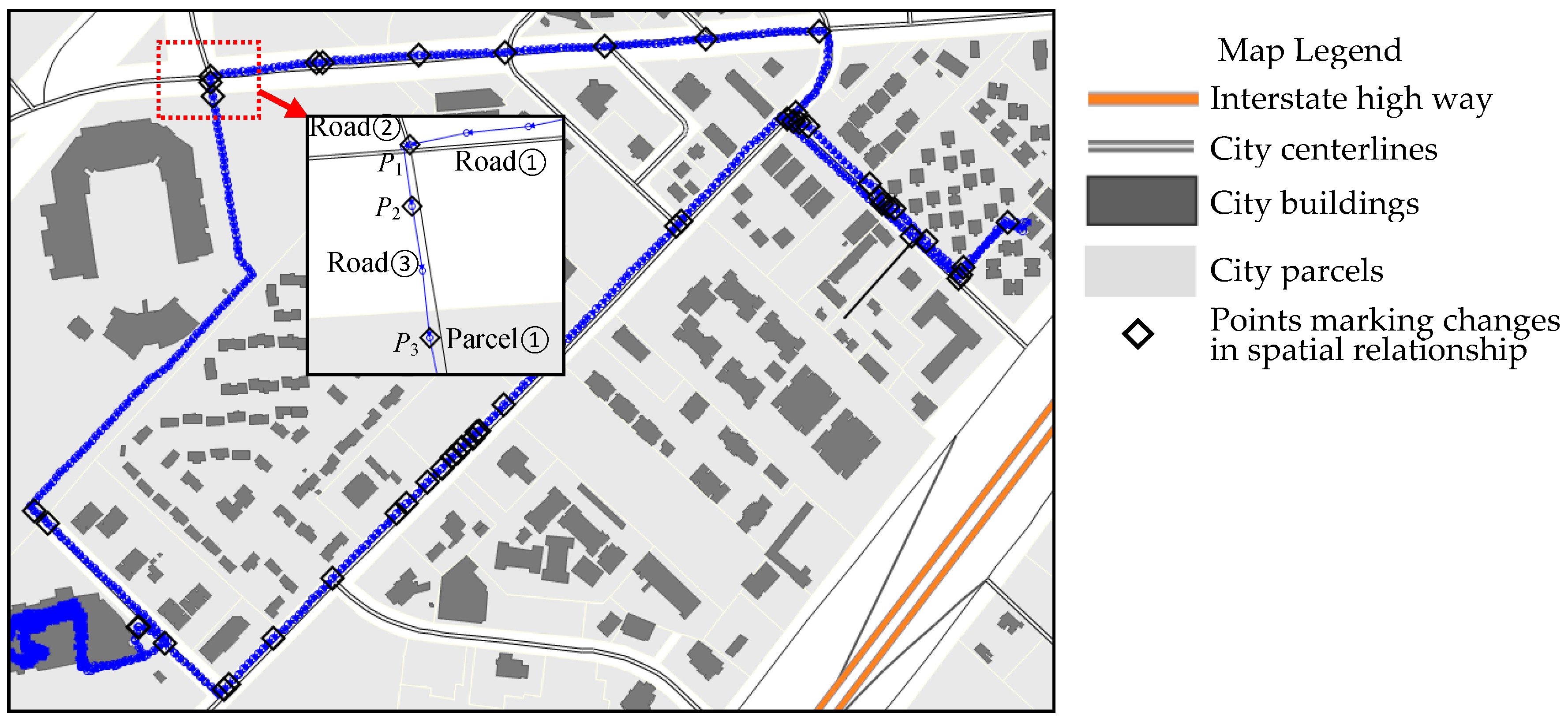
2.3. Constraint of Spatial Relationship
The spatial relationships between GPS trajectory and geography features (including roads and off-road places such as buildings or open markets) are important for understanding human activities. Thus, the GPS points that mark changes of such spatial relationships should be preserved during trajectory simplification.
Points marking changes in spatial relationship: This constraint requires that the points that mark topological changes between a GPS trajectory and geographical features be preserved. Keeping these points where the topological relationship between a trajectory line and geographical features changes are critical for describing not only the geometry of trajectory but also the related spatial-temporal activities of a subject. These points may indicate transition along a journey from one road onto another or from moving to staying activities (e.g., location points P1, P2, and P3, as illustrated in Figure 3). For transition between moving and staying activities, pending on algorithms used, spatial-relationship constraint may be observed together with time constraint, for the points marking topology change may also mark the starting or ending points for a staying activity.
| The relationships of P1, P2 and P3 to other features. | |
| Characteristic Points | Relationships to Others |
| P1 | road ①, road ② |
| P2 | road ③ |
| P3 | road ③, parcel ① |
2.4. Elevation Constraint
Another piece of information from GPS data is elevation, with which we can determine whether the GPS trajectory for moving object underground, on the ground, or flying in the air. Combining elevation with speed information will allow us to better understand the context of spatial-temporal activities as well as moving or transportation mode. Thus, points with distinct value of elevation should be preserved.
Points of extreme elevation: This constraint requires that the GPS points of local highest or lowest elevation values be preserved during GPS trajectory simplification. These points are likely good indicators of actual activities places and travel mode.
2.5. Additional Geometry Constraint
Although traditional DP algorithm considers geometry properties, points with important geometric characteristics may get deleted occasionally. Therefore, additional constraints are necessary to help better preserve geometry properties. For example, partial maximum distance (PMD) method is used for map generalization to preserve a point that is furthest away from its related road segment; geometry shape of a trajectory at a local segment is better preserved this way. Note that PMD is different from DP’s recursive selection of critical points (Figure 1) as PMD seeks to preserve points that are furthest from real-world road segments not from line segments in a graphic representation of a trajectory.
Points of local maximum distance: This constraint requires that a GPS point that is furthest away from its related road segment be preserved.
It is important to note that these ESTCs as discussed above are not meant to exclusively cover all important aspects of GPS trajectory data. By no means any set of ESTCs can include all possible scenarios. Furthermore, a particular GPS trajectory simplification must implement the constraints by considering particular environment context and traveling situation. The parameters for constraints must be defined to reflect the peculiarity of a trajectory. For example, for a ground transportation, an extremely large speed such as 200 miles per hour is more likely a data error than an extreme speed to preserve under “speed constraint”. Similarly, elevation constraint may not apply when simplifying a trajectory that known to occur on a relative flat landscape.
Furthermore, note that GPS data cleaning, such as that described in Schuessler and Axhausen [31], should be performed on raw data before conducting trajectory simplification. For the GPS empirical datasets used in this paper, Lagrange fitting algorithm was applied to correct apparent errors in data before ESTC-EDP was used. Cleaning raw GPS trajectory data will reduce the chances for incorrectly keeping spurious locations as critical points during trajectory simplification.
3. Evaluating the Effectiveness of Trajectory Simplification
In addition to geometry properties, how the locations are connected through time (i.e., speed) is essential for describing a trajectory. Moreover, the change of speed through time describes the dynamics of moving status throughout a trajectory. Hence, together with geometry, speed and the change of speed throughout a trajectory uniquely define a trajectory. We use the term, speed–time profile, to refer to speed and changes of speed throughout a trajectory. An effective GPS trajectory simplification preserves the geometry of a trajectory so that location, orientation, and shape are kept as close to the original data as possible; it also preserves the speed–time profile of a trajectory so that there is minimum difference between pre- and post-simplified trajectory data.
A speed–time graph of a trajectory uses y-axis to show speed and x-axis time to describe speed and its variation through time. A speed–time graph presents a holistic picture about how fast/slow a subject travel at any time during a trajectory (Figure 4a). A trajectory simplification process would drop some points from the original GPS dataset, but the speed–time profile as revealed by a speed–time graph should reveal minimum change for post-simplification data compared to pre-simplification data.
Using the speed–time graph in Figure 4a as an example, the speeds at points P1, P2 and P3 are equivalent. If point P2 is deleted through a trajectory simplification, there will be no speed information loss as the speed at point P2 can be accurately interpolated based on speed data for P1 and P3. However, the situation is different for points P3, P4 and P5. If point P4 is deleted, the original trajectory segment of P3–P4–P5 will be recorded as P3–P5 (Figure 4b). In this case, it will be quite a challenge to interpolate accurately the speed at point P4 based on speed information for P3 and P5. If P'4 is generated through interpolation, the gap between P4 and P'4 indicates an error, and it measures the magnitude of speed information loss, referred to as speed loss in this paper.
When simplifying a complete trajectory, we can calculate speed loss for every point that was dropped. Dividing the total speed loss for all removed points by the total number of points removed will generate average speed loss. Relative average speed loss is the percentage of average speed loss from trajectory simplification to average speed of a trajectory. These indicators can be used to assess the effectiveness of a trajectory simplification algorithm.
4. Applying ESTC-EDP on Experimental Data
4.1. Two Trajectory Data
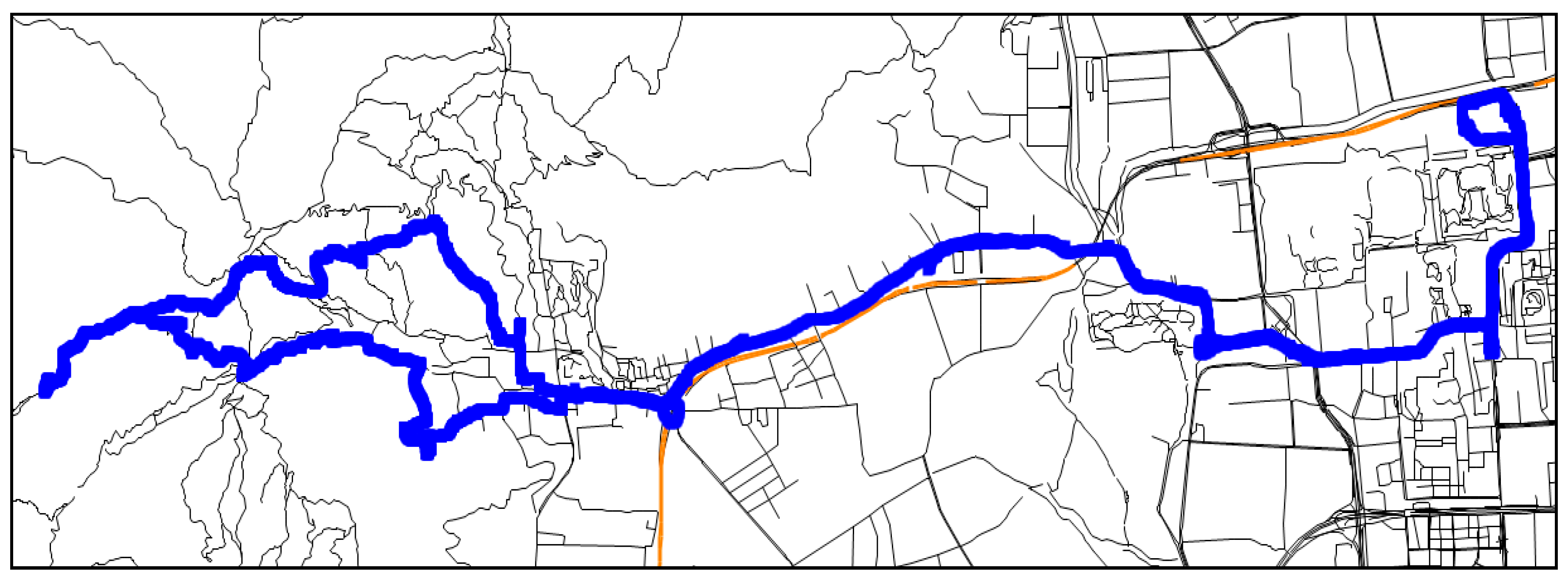
The experimental data involve two GPS trajectories collected in the city of San Marcos, Texas. The first dataset was gathered for walking (Figure 5), and the second dataset was for a mixed transportation consisting of walking and bus riding (Figure 6). The background map was downloaded from San Marcos city website [32]. The total distance for the walking trajectory is about one mile while that for the second trajectory is about eight miles. As can be seen from Figure 5 and Figure 6, the GPS points are too dense to be clearly illustrated on a map. Simplifying the GPS trajectory data will help both map representation and data analysis. Note that before applying trajectory simplification and in order to minimize noise that may be introduced by errors in the original GPS data, Lagrange fitting algorithm was applied to clean and prepare the empirical trajectory data.
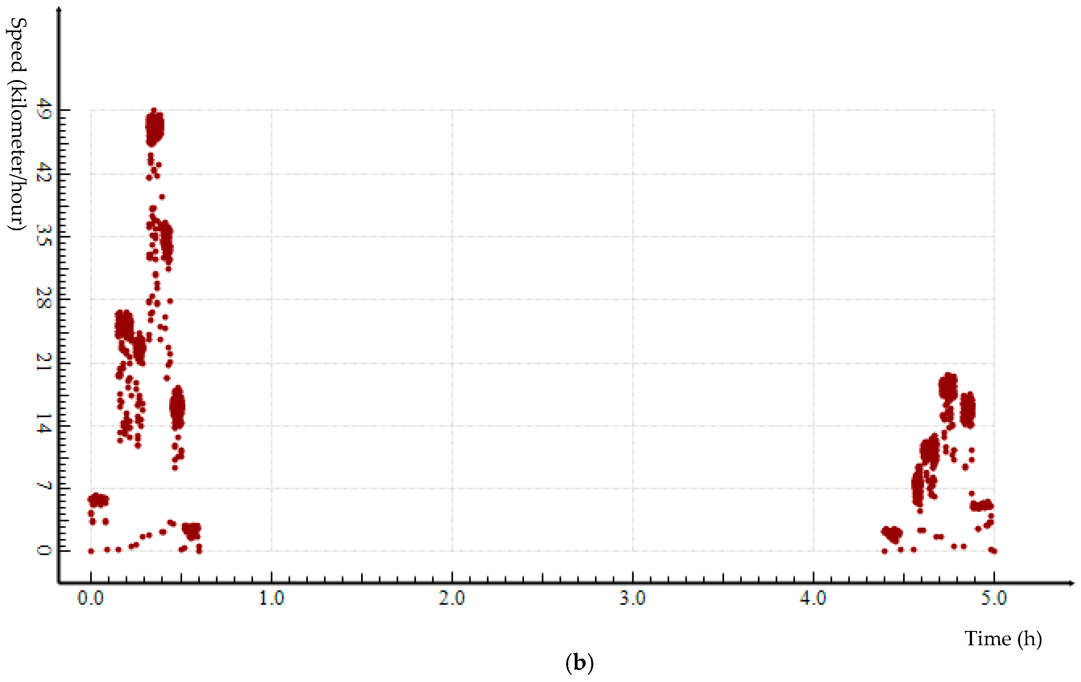
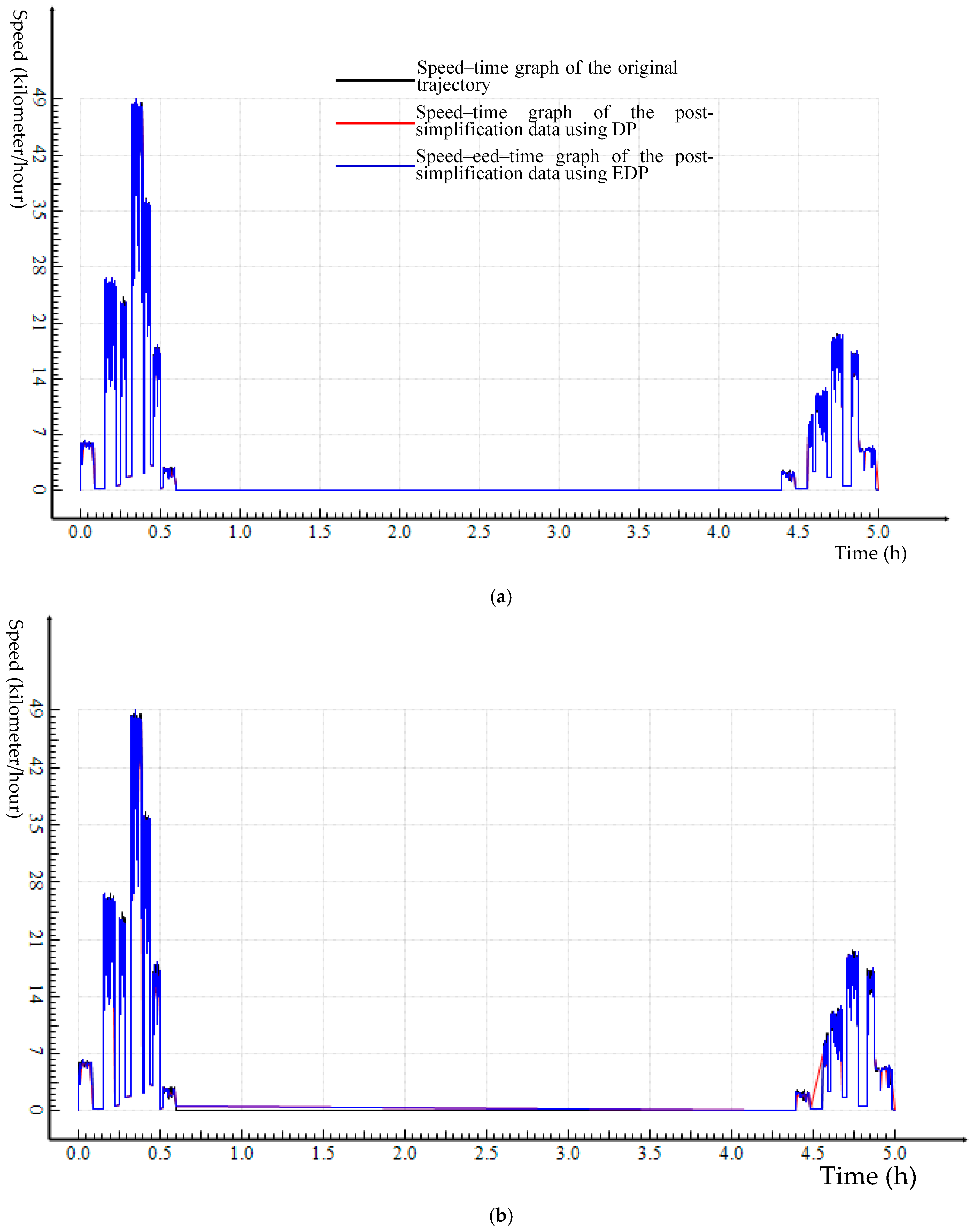
To capture the speed dynamics of Trajectory 1, a speed–time graph is created (see Figure 7a). The X-axis shows time and the Y-axis shows speed. This figure provides a whole picture of the speed–time profile of this trajectory, including maximum and minimum speed, total travel time, and the distribution of speed in time sequence. Figure 7b shows the speed–time graph for Trajectory 2.
4.2. Trajectory Simplification Applied on Trajectory 1
Both DP and ESTC-EDP trajectory simplification were applied to the two trajectory datasets. Note that the EDP simplification preserves geometry properties following traditional DP; it further adopts a set of ESTCs as discussed in Section 2 of the paper to preserve the critical points along a trajectory in order to correctly represent spatial-temporal movement.
Figure 8 highlights the critical points along Trajectory 1. Among the 1141 GPS points in the original dataset, a total of 90 critical points were identified using ESTCs. Table 1 reports on the preservation of GPS points after applying DP and EDP simplification on Trajectory 1 data using different distance thresholds. The distance threshold dx for geometry properties (see Figure 1) was set to increase from 1-m to 100-m. We understand that, for a practical trajectory simplification, the selection of a distance threshold is key for the final results. Abundant research exists that investigates the best strategies for identifying such a threshold. Since the experiments reported here is to compare the simplification results from DP and EDP across a spectrum of thresholds, we focus on examining possible relationship between threshold distance and critical point preservation.
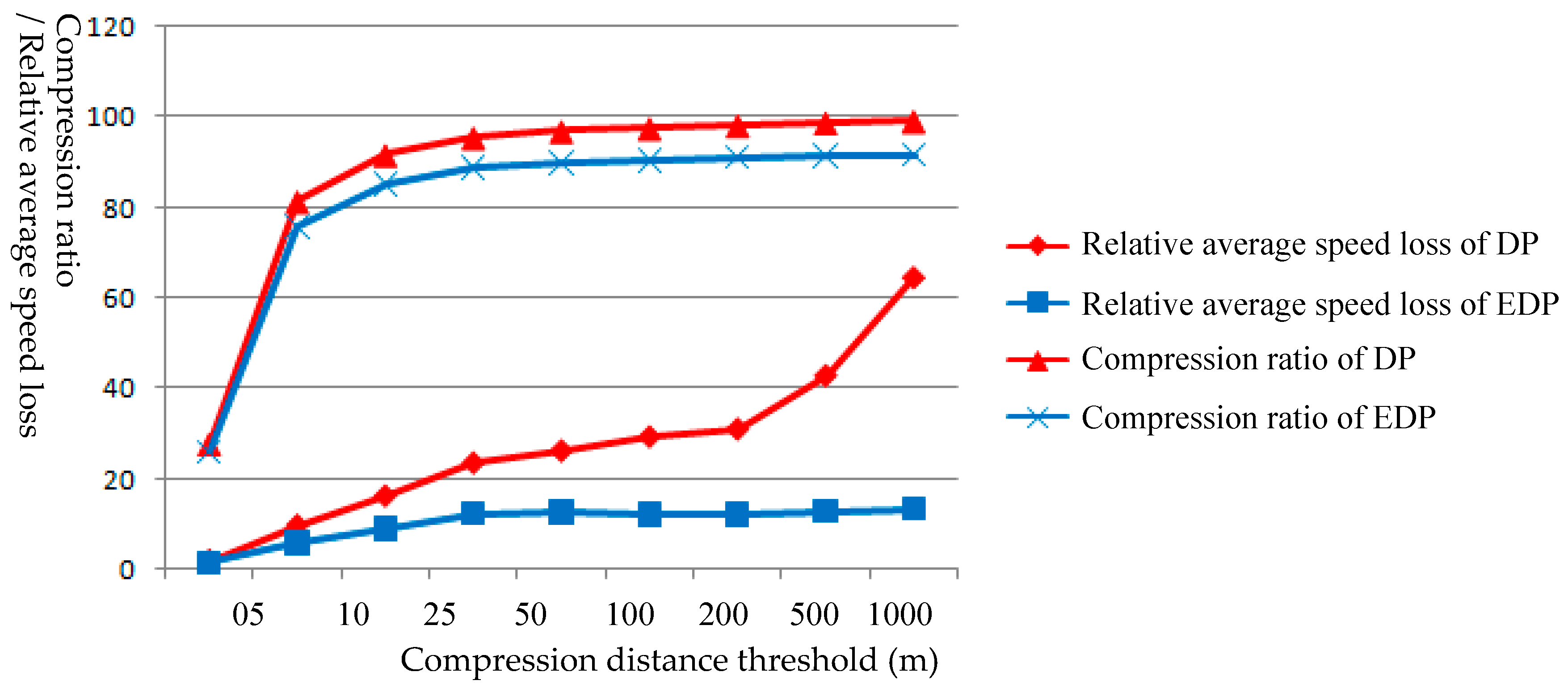
Compression ratio measures the percentage of points deleted through a trajectory simplification. Note that the loss of critical points by DP algorithm as compared to EDP continuously increases with the increase of distance threshold (Table 1). The number of lost critical points by DP and the overall compression ratio for both DP and EDP start to converge at distance threshold of 10-m.
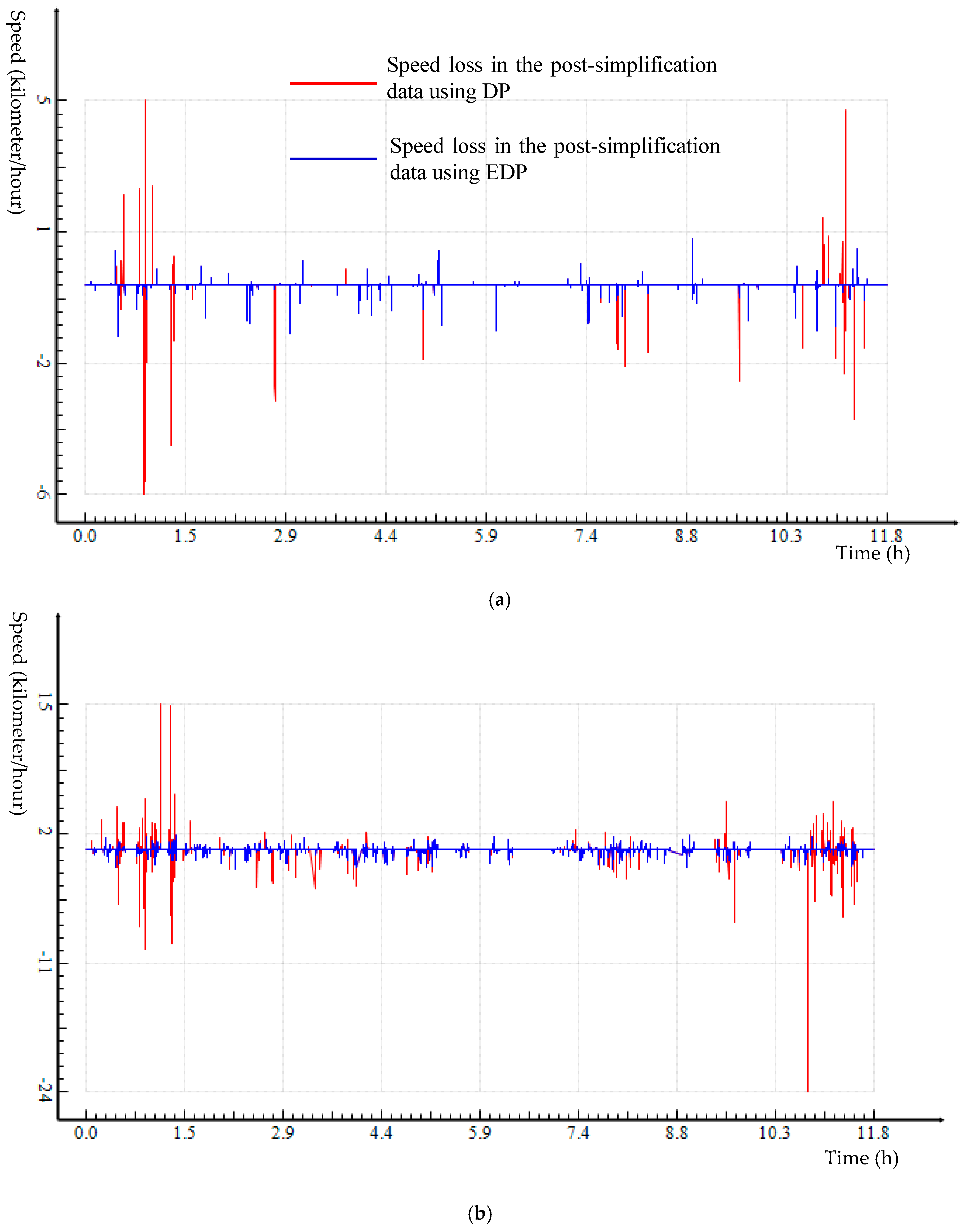
In addition to the preservation of critical points, speed–time graph was used to compare the pre- and post-simplification datasets. Speed loss was also examined. Figure 9 shows speed–time graphs of the post-simplification datasets from DP and EDP as compared to the original Trajectory 1 dataset; the distance threshold increases from of 1-m, to 5-m, 10-m, and 25-m respectively. The panels in Figure 10 show speed loss by the two simplification algorithms for Trajectory 1 data with the same set of thresholds. The graphs in both Figure 9 and Figure 10 clearly show that, as distance threshold increases, EDP outperforms DP more by introducing a narrower gap between the original speed–time graph and the post-simplification counterpart, and by leading to less speed loss.
Table 2 reports on the quantity of speed loss from trajectory simplification by DP and EDP algorithms. It can be seen that EDP proves to have less speed loss compared to DP algorithm; the difference between DP and EDP simplification results becomes more apparent as distance threshold increases. Further, as the distance threshold increases, the average speed loss and relative average speed loss generally increase, but the magnitude of loss tends to converge in the EDP results.
4.3. Trajectory Simplification Applied on Trajectory 2
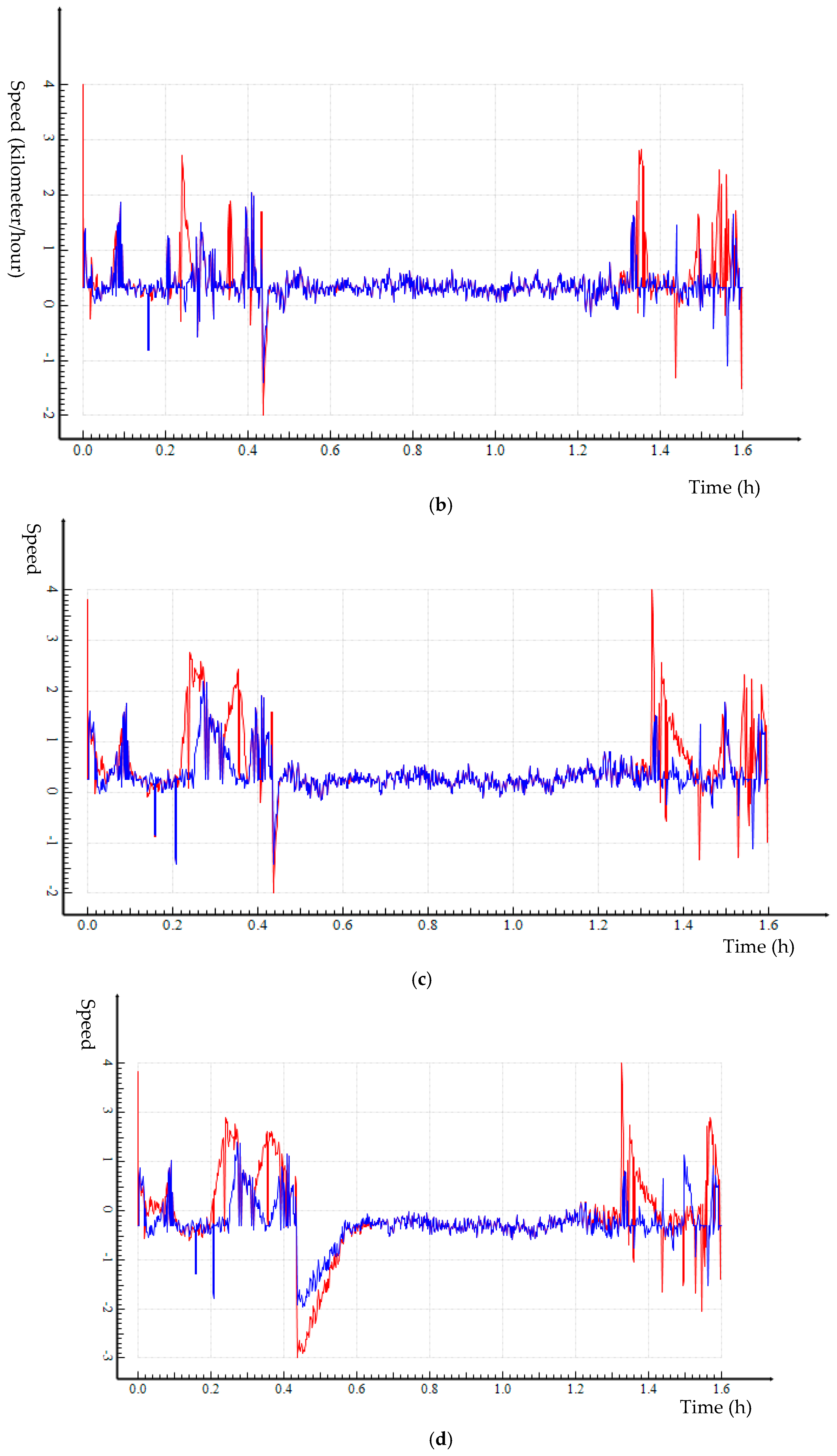
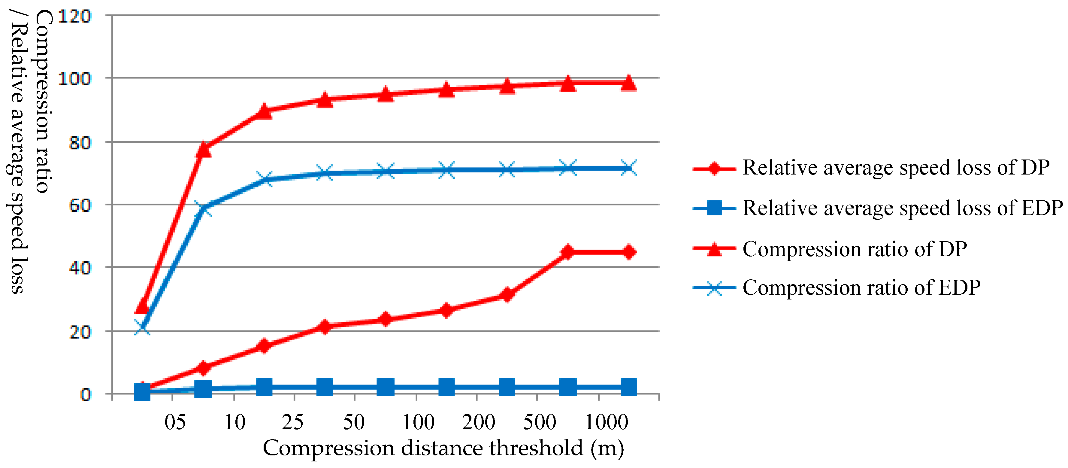
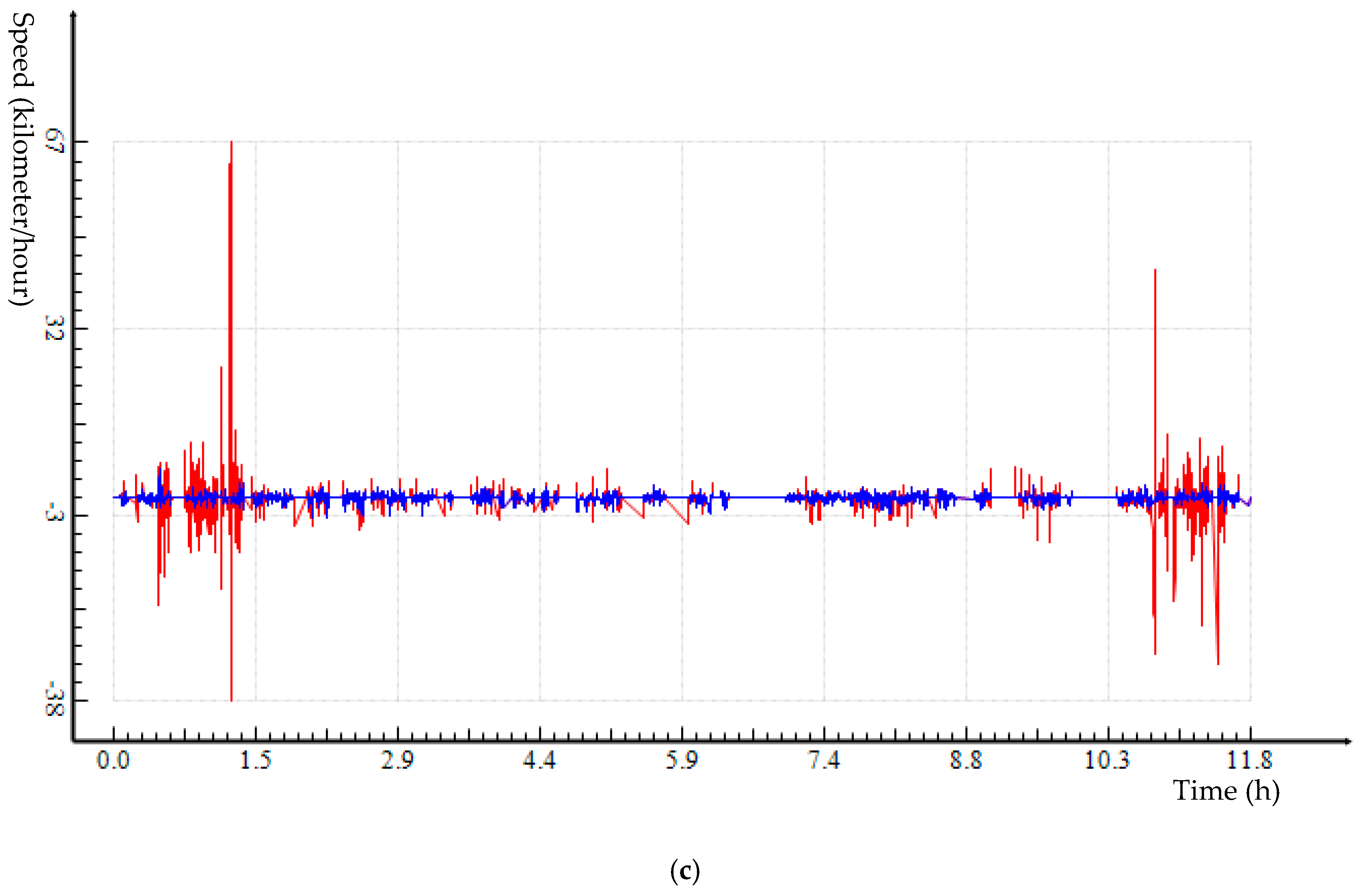
Experiments were done with Dataset 2 using DP and EDP algorithms, respectively. Among the 2010 points, 568 were identified as critical points by ESTCs. Table 3 reports on the numbers of points preserved through simplification and the loss of critical points. Similar to the results for Trajectory 1 dataset, the loss of critical points by DP algorithm continuously increases as distance threshold increases, but the number of lost critical points tends to converge eventually. The graphs in Figure 11 and Figure 12 show speed–time graph and speed loss for the original Trajectory 2 dataset and the post-simplification datasets from DP and EDP as distance threshold was set to be 1-m, 5-m, 10-m, and 25-m. Trajectory 2 contains a segment of a few hours with no spatial movement, which is clearly reflected by the speed–time graphs in Figure 11. Both DP and EDP are relatively accurate when simplifying the staying segment of Trajectory 2. However, similar to the analyses of Trajectory 1 dataset, EDP outperforms DP more as the distance threshold increases. This is more apparent when checking the speed loss graphs (Figure 12).
Table 4 reports on the quantity of speed loss when DP and EDP algorithms were applied to Dataset 2. As distance threshold increases, both average speed loss per point and relative average speed loss increase; however, the magnitude of loss start to converge clearly for EDP results at a distance threshold of 10-m.
5. Conclusions and Discussion
To effectively simplify a very large GPS trajectory dataset, traditional line generalization algorithms can be enhanced by a set of spatial-temporal constraints so that both geometrical and non-geometrical characteristics that are essential for defining and describing spatial-temporal movement and the related travel behavior can be preserved. Considering that variations exist regarding trajectory environment, moving modes, subjects’ behavior, etc., this paper discusses enhanced spatial-temporal constraints (ESTC) from five aspects: speed constraint, time constrain, constraint of spatial relationship, elevation constraint, and additional geometry constraint. The implementation of these constraints for a trajectory must reflect the peculiarity of spatial-temporal and individual activity context.
Both Douglas–Peuker (DP) and Enhanced DP (EDP) algorithms were applied to two empirical trajectory datasets that were collected by the researchers. A range of distance thresholds was used for trajectory simplification. It is clear that, compared to DP, EDP trajectory simplification performs consistently better across the distance thresholds for both trajectory datasets. EDP preserves all critical points through implementing the various ESTCs (Table 1 and Table 3); keeps the speed profile of trajectory closer to the original data (Figure 9 and Figure 11); and controls speed loss better (Table 2 and Table 3, and Figure 10 and Figure 12).
We noticed that literature has started seeing attempts seeking to preserve speed during trajectory simplification. For example Ying and Su [33] proposed an approach for trajectory simplification with velocity preservation. However, their method only ensures that the velocity difference between a simplified trajectory and the original data is below a threshold. They failed to consider other aspects that are important for a trajectory, which can be preserved by our ESTC-EDP method through the five spatial-temporal constraints as explained in Section 2. A simplified trajectory following [32] may fail to catch the movement of a trajectory that enters and/or exists a market or a public park if there is no big speed change in the process; similarly, it may mistakenly delete the elevation peak point along a trajectory. Our ESTC-EDP method enforces the preservation of these critical points along a trajectory.
To further the discussion on comparing the effectiveness of DP and EDP, Figure 13 and Figure 14 are created to show the change of trajectory data compression ratio and relative average speed loss when the distance threshold for simplification increases. For illustration purpose, we have reported in the two graphs very large distance thresholds for the purpose of showing trend; these thresholds are not likely to be used in real cases. We can see that, despite that compression ratio has a converging trend for both DP and EDP algorithms, relative average speed loss of DP and EDP algorithms show different patterns. The relative average speed loss for DP simplification continues to increase as distance threshold increases, while that for EDP simplification starts to stay stable at a relatively small value.
It can also be observed in Figure 13 and Figure 14 that when DP and EDP methods are applied to both trajectory datasets, the compression ratio of both approaches converge to a level after a certain distance threshold, around 25-m for the empirical datasets in the experiments. This threshold may vary across different landscapes as well as GPS data qualities. It is an important parameter to know for deciding on trajectory simplification parameters. Note that the compression ratio from DP algorithm is expected to be larger than that from EDP algorithm, as EDP uses ESTCs to enforce the preservation of critical points in addition to the geometrically essential points along a trajectory. However, the compression ratios from DP and EDP are more similar for Trajectory 1 than those for Trajectory 2. This may indicate that EDP simplification for Trajectory 1 produced results more similar to that from DP, and EDP algorithm is more effective for simplification of Trajectory 2 dataset. This could be due to the fact that travel mode for Trajectory 1 is relative simple with mostly walking and staying while Trajectory 2 contains a lot of bus moving-and-stop and traffic speed variation. It is also important to notice that, with more critical points preserved for Trajectory 2 by EDP, the average speed loss is noticeably smaller for Trajectory 2 simplification than for Trajectory 1. This suggests that EDP simplification have greatly improved the trajectory simplification of Dataset 2, for which critical points are better preserved and average speed loss better controlled.
We recognize that more experiments are needed to test for the effectiveness of the proposed ESTC-EDP simplification method. The two trajectories used for case studies in this paper were collected by the authors in very similar environment settings (i.e., the same city). To further illustrate the effectiveness of ESTC-EDP, we applied it on a secondary trajectory dataset that were collected in a different place. The analyses and results are reported in Appendix A. Similar to the findings reported above, ESTC-EDP is proven to be more effective for trajectory simplification.
Like any other studies, this reported trajectory simplification approach and the empirical analyses are not without limitations. First, the empirical trajectory datasets used here are limited to built environment and are all intra-city movements. Future studies should further investigate how the effectiveness of EDP may be related to the different aspects of trajectories, including topography, land use patterns, traffic variation, transportation modes and mixture of modes, and frequency of staying-moving transition. With ESTC to be designed to reflect the environment for and the spatial-temporal movement variations of a trajectory, EDP is effective in considering the peculiarity of more complexed settings and trajectories. Second, systematic design should be applied to collect trajectory datasets to enable further comparison of EDP and DP simplification at selected context settings. Speed–time graph and relative average speed loss can be used as measures for the effectiveness of a trajectory simplification.
Acknowledgments
The research was conducted when H. Qian was a visiting scholar at Texas State University. Qian’s research was also sponsored by the National Natural Science Foundation of China, No. 41571442 (2016–2019) and No. 41171305 (2012–2015).
Author Contributions
Y.L. conceived and designed the research; H.Q. and Y.L. designed the experiments; H.Q. performed the experiments; H.Q. and Y.L. analyzed the data; and Y.L. and H.Q. wrote the paper.
Conflicts of Interest
The authors declare no conflict of interest. The founding sponsors had no role in the design of the study; in the collection, analyses, or interpretation of data; in the writing of the manuscript, and in the decision to publish the results.
Appendix A: ESTC-EDP Applied on a Secondary GPS Trajectory Dataset
We applied the proposed ESTC-EDP trajectory simplification method to a secondary dataset of GPS trajectory. Microsoft Research Asia’s Geolife project collected a series of GPS trajectory data by 182 individuals in a period of over five years (from April 2007 to August 2012). More information about these data can be found at [34]. We applied DP and ESTC-EDP methods to one of the GPS trajectories (Figure A1), which is identified in the dataset as “001/Trajectory/20081024234405.plt”. This trajectory includes 7076 recorded points (Figure A1). Considering paper length, we report here only the simplification results from three distance thresholds (0.1-m, 1-m, and 10-m) and the corresponding speed–loss figures. Table A1 and Table A2 summarize the results of point preservation by both traditional DP simplification and ESTC-EDP simplification. Speed loss graphs in Figure A2 show that, when the distance threshold of 1-m is applied, speed loss from DP simplification is much larger than that from ESTC-EDP. With a distance threshold of 10-m, the speed loss of EDP algorithm remains low (Figure A2c).
Figure A1.
A GPS trajectory with 7076 points from GeoLife Project dataset of Microsoft Research Asia.
Figure A1.
A GPS trajectory with 7076 points from GeoLife Project dataset of Microsoft Research Asia.


Table A1.
Points and critical points preserved by DP and EDP algorithms.
| Distance Threshold (m) | DP | EDP | Number of Critical Points Deleted by DP Incorrectly | ||
|---|---|---|---|---|---|
| Points Remained | Compression Ratio (%) | Points Remained | Compression Ratio (%) | ||
| 0.1 | 6797 | 3.94 | 6841 | 3.32 | 44 |
| 1 | 5669 | 19.88 | 5942 | 16.03 | 273 |
| 10 | 2407 | 65.98 | 3571 | 49.53 | 1164 |
Table A2.
Speed loss of DP and EDP simplification with different distance thresholds.
| Distance Threshold (m) | DP | EDP | ||||
|---|---|---|---|---|---|---|
| Total Speed Loss (km/h) | Average Speed Loss (km/h) | Relative Average Speed Loss (%) | Total Speed Loss (km/h) | Average Speed Loss (km/h) | Relative Average Speed Loss (%) | |
| 0.1 | 195.096 | 0.028 | 0.296 | 64.648 | 0.0091 | 0.098 |
| 1 | 1055.47 | 0.15 | 1.6 | 419.07 | 0.059 | 0.635 |
| 10 | 7004.67 | 0.989 | 10.63 | 2329.49 | 0.329 | 3.534 |
Figure A2.
Speed loss in the post-simplification data using DP and EDP algorithms with a distance threshold of: 0.1-m (a); 1-m (b); and 10-m (c).
Figure A2.
Speed loss in the post-simplification data using DP and EDP algorithms with a distance threshold of: 0.1-m (a); 1-m (b); and 10-m (c).

References
- Muckell, J.; Olsen, P.W., Jr.; Hwang, J.-H.; Lawson, C.T.; Ravi, S.S. Compression of trajectory data: A comprehensive evaluation and new approach. GeoInformatica 2014, 18, 435–460. [Google Scholar] [CrossRef]
- Long, C.; Wong, R.C.-W.; Jagadish, H.V. Direction-preserving trajectory simplification. Proc. VLDB Endow. 2013, 6, 949–960. [Google Scholar] [CrossRef]
- Givsudan, J.; Abdelguerfi, M.; Shaw, K.B.; Ladner, R.V. The 2-3TR-tree, a trajectory-oriented index structure for fully envolving valid-time spatio-temporal datasets. In Proceedings of the 10th SIGSPATIAL International Conference on Advances in Geographic Information Systems (ACM-GIS), McLean, VA, USA, 8–9 November 2002; pp. 29–34. [Google Scholar]
- Agarwal, P.K.; Guibas, L.J.; Edelsbrunner, H.; Erickson, J.; Isard, M.; Har-Peled, S.; Hershberger, J.; Jensen, C.; Kavraki, L.; Koehl, P.; et al. Algorithmic issues in modeling motion. ACM Comput. Surv. 2002, 34, 550–572. [Google Scholar] [CrossRef]
- Giannotti, F.; Nanni, M.; Pinelli, F.; Pedreschi, P. Trajectory pattern mining. In Proceedings of the 13th International Conference on Knowledge Discovery and Data Mining (ACM-KDD), San Jose, CA, USA, 12–15 August 2007; pp. 330–339. [Google Scholar]
- Prior, J.M. Satellite Communications Systems Buyer’s Guide; British Antarctic Survey: Cambridge, UK, 2008. [Google Scholar]
- Zhu, H.; Su, J.; Ibarra, O.H. Trajectory queries and octagons in moving object databases. In Proceedings of the 11th Conference on Information and Knowledge Management (CIKM), McLean, VA, USA, 4–9 November 2002; pp. 413–421. [Google Scholar]
- Bellman, R. On the approximation of curves by line segments using dynamic programming. Commun. ACM 1961, 4, 284. [Google Scholar] [CrossRef]
- Douglas, D.H.; Peucker, T.K. Algorithms for the reduction of the number of points required to represent a line or its caricature. Can. Cartogr. 1973, 10, 112–122. [Google Scholar] [CrossRef]
- Muller, J. Fractal and automated line generalization. Cartogr. J. 1987, 24, 27–34. [Google Scholar] [CrossRef]
- Wang, Q.; Wu, H. The Fractal Description and Auto-Generalization Research of Map Information; The Publishing House of Wuhan Technical University of Surveying and Mapping: Wuhan, China, 1998; pp. 2–11. [Google Scholar]
- Visvalingam, M.; Whyatt, J. The Douglas-Peucker algorithm for line simplification: reevaluation through visualization. Comput. Graph. Forum 1990, 9, 213–228. [Google Scholar] [CrossRef]
- Li, Z.; Openshaw, S. Algorithms for automated line generalization based on a natural principle of objective generalization. Int. J. Comput. Geom. 1992, 6, 373–390. [Google Scholar]
- Peng, W.; Muller, J.C. A dynamic decision tree structure supporting urban road network automated generalization. Cartogr. J. 1996, 33, 5–10. [Google Scholar] [CrossRef]
- Guo, Q.S. A progressive line simplification algorithm. J. Wuhan Tech. Univ. Surv. Mapp. 1998, 1, 52–56. [Google Scholar]
- Qian, H.Z.; Wu, F.; Chen, B.; Wang, J.-Y. Simplifying line with oblique dividing curve method. Acta Geod. Cartogr. Sin. 2007, 11, 443–456. [Google Scholar]
- Gudmundsson, J.; Katajainen, J.; Merrick, D.; Ong, C.; Wolle, T. Compressing spatio-temporal trajectories. Comput. Geom. 2009, 42, 825–841. [Google Scholar] [CrossRef]
- Potamias, M.; Patroumpas, K.; Sellis, T. Sampling trajectory streams with spatiotemporal criteria. In Proceedings of the IEEE 18th International Conference on Scientific and Statistical Database Management, Washington, DC, USA, 3–5 July 2006; pp. 275–284. [Google Scholar]
- Muckell, J.; Hwang, J.-H.; Patil, V.; Lawson, C.T.; Ping, F.; Ravi, S.S. SQUISH: An online approach for GPS trajectory compression. In Proceedings of the 2nd International Conference on Computing for Geospatial Research & Applications, ACM, Washington, DC, USA, 13–25 May 2011; pp. 1–13. [Google Scholar]
- Chen, M.; Xu, M.; Franti, P. A Fast O(N) Multiresolution Polygonal Approximation Algorithm for GPS Trajectory Simplification. IEEE Trans. Image Process. 2012, 21, 2770–2785. [Google Scholar] [CrossRef] [PubMed]
- Birnbaum, J.; Meng, H.-C.; Hwang, J.-H. Similarity-Based Compression of GPS Trajectory Data. In Proceedings of the Fourth International Conference on IEEE Computing for Geospatial Research and Application (COM. Geo), San Jose, CA, USA, 22–24 July 2013; pp. 92–95. [Google Scholar]
- Nibali, A.; He, Z. Trajic: An Effective Compression System for Trajectory Data. IEEE Trans. Knowl. Data Eng. 2015, 27, 3138–3151. [Google Scholar] [CrossRef]
- Tobler, W.R. Numerical Map Generalization and Notes on the Analysis of Geographical Distributions (Michigan Inter-University Community of Mathematical Geographers, Discussion Paper No. 8); Department of Geography, University of Michigan: Ann Arbor, MI, USA, 1966. [Google Scholar]
- Meratnia, N.; Rolf, A. Spatiotemporal compression techniques for moving point objects. In Advances in Database Technology-EDBT 2004; Springer: Berlin/Heidelberg, Germany, 2004; pp. 765–782. [Google Scholar]
- Sun, P.; Xia, S.; Yuan, G.; Li, D. An Overview of Moving Object Trajectory Compression Algorithms. Math. Probl. Eng. 2016, 2016, 1–13. [Google Scholar] [CrossRef]
- Lu, Y. Detecting Travel Patterns and Deviation from Routine. In Proceedings of the 107th Annual Meeting of Association of American Geographers, Seattle, WA, USA, 12–16 April 2014; pp. 12–16. [Google Scholar]
- Schmid, F.; Richter, K.-F.; Laube, P. Semantic trajectory compression. In Advances in Spatial and Temporal Databases; Springer: Berlin/Heidelberg, Germany, 2009; pp. 411–416. [Google Scholar]
- Chen, Y.; Jiang, K.; Zheng, Y.; Li, C.; Yu, N. Trajectory simplification method for location-based social networking services. In Proceedings of the 2009 International Workshop on Location Based Social Networks, Seattle, WA, USA, 3 November 2009; pp. 33–40. [Google Scholar]
- Gong, H.M.; Chen, C.; Bialostozky, E.; Lawson, C.T. A GPS/GIS method for travel mode detection in New York City. Comput. Environ. Urban Syst. 2012, 36, 131–139. [Google Scholar] [CrossRef]
- Wan, N.; Ge, L. Life-space characterization from cellular telephone collected GPS data. Comput. Environ. Urban Syst. 2013, 39, 63–70. [Google Scholar] [CrossRef]
- Schuessler, N.; Kay, A. Processing raw data from global positioning systems without additional information. Transp. Res. Rec. J. Transportation Res. Board 2009, 2105, 28–36. [Google Scholar] [CrossRef]
- San Marcos Map Library. Available online: http://www.ci.san-marcos.tx.us/800/Map-Library (accessed on 27 October 2017).
- Ying, J.J.C.; Su, J.H. On Velocity-Preserving Trajectory Simplification. In Intelligent Information and Database Systems. ACIIDS 2016. Lecture Notes in Computer Science; Nguyen, N.T., Trawiński, B., Fujita, H., Hong, T.P., Eds.; Springer: Berlin/Heidelberg, Germany, 2016; Volume 9622, pp. 241–250. [Google Scholar]
- GeoLife GPS Trajectories. Available online: https://www.microsoft.com/en-us/download/details.aspx?id=52367 (accessed on 27 October 2017).
Figure 1.
Schematic diagram of DP algorithm.
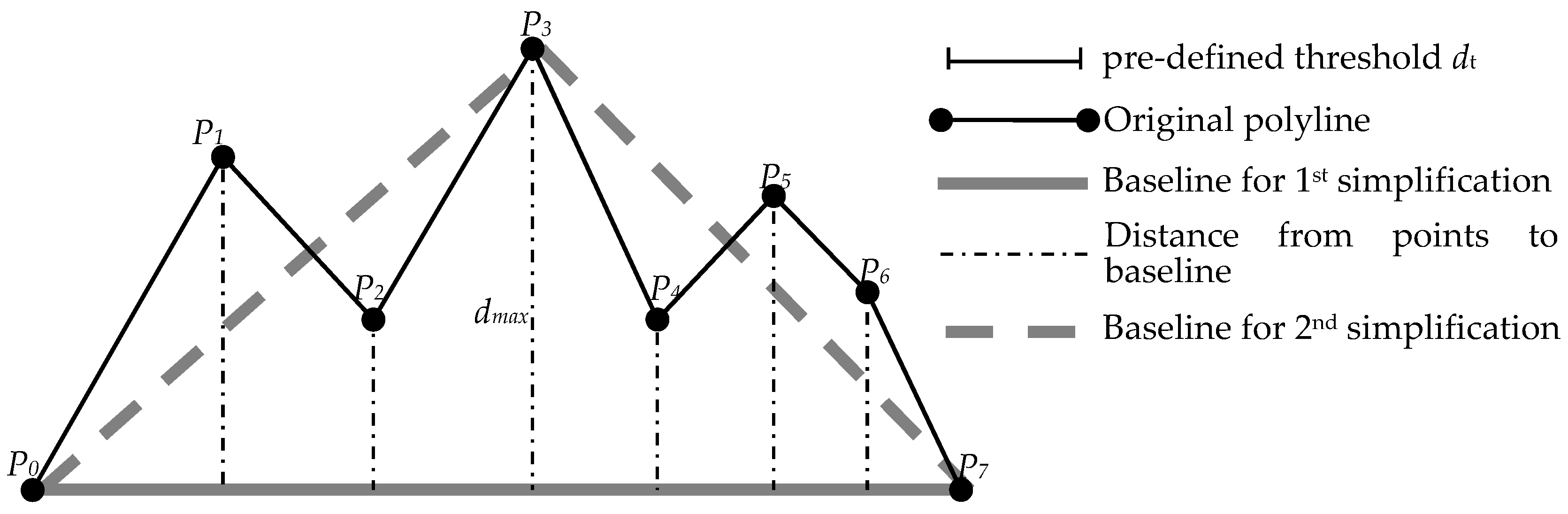
Figure 2.
Time constraint must be applied when separating passing points from stay points.
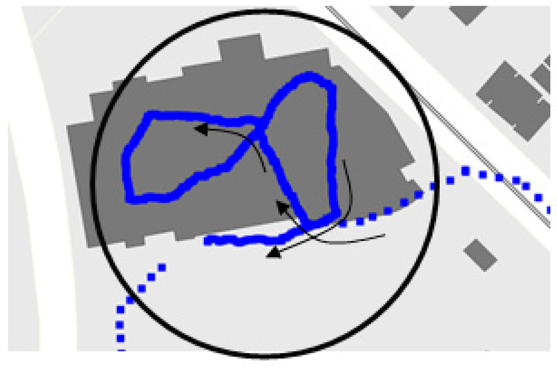
Figure 3.
Critical points marking changes of spatial relationship. Note: The relationships of P1, P2 and P3 to other features are different in the above map, which are summarized in the table below. P1 are spatially related with road and road ②. P2 is only related to road ③. P3 are spatially related to road ③ and parcel ①.

Figure 4.
Speed loss through trajectory simplification: (a) speed–time graph of a trajectory; and (b) speed loss at P4 with incorrect trajectory simplification that fails to preserve P4.
Figure 4.
Speed loss through trajectory simplification: (a) speed–time graph of a trajectory; and (b) speed loss at P4 with incorrect trajectory simplification that fails to preserve P4.
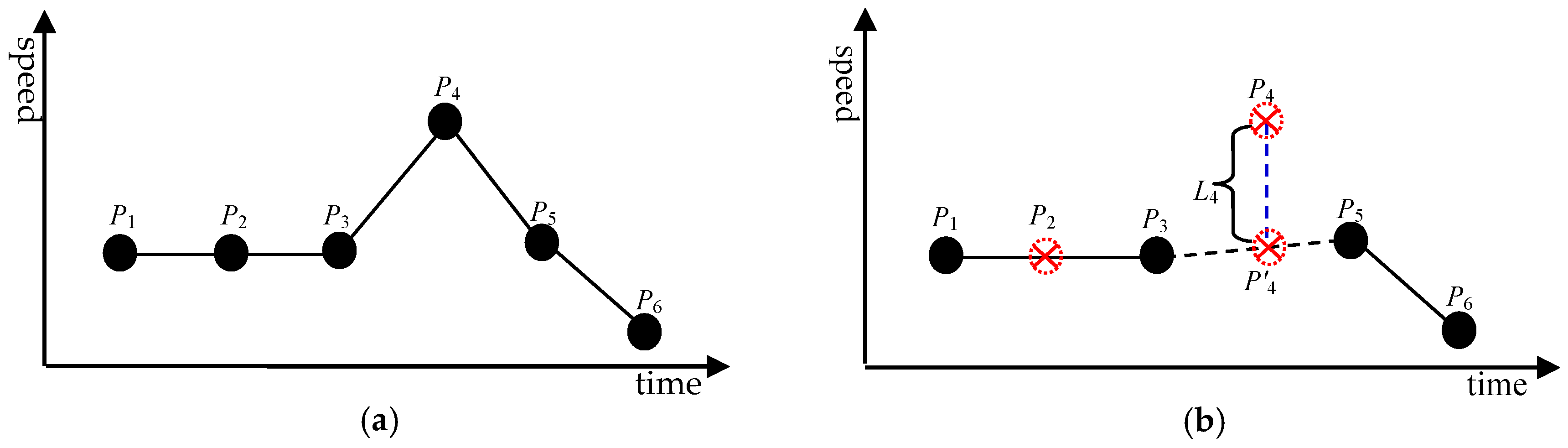
Figure 5.
A GPS trajectory of 1141 points collected for a walking trip. It was a round trip following the arrows, starting from point A, arriving at point B, and back to A by a different route.
Figure 5.
A GPS trajectory of 1141 points collected for a walking trip. It was a round trip following the arrows, starting from point A, arriving at point B, and back to A by a different route.

Figure 6.
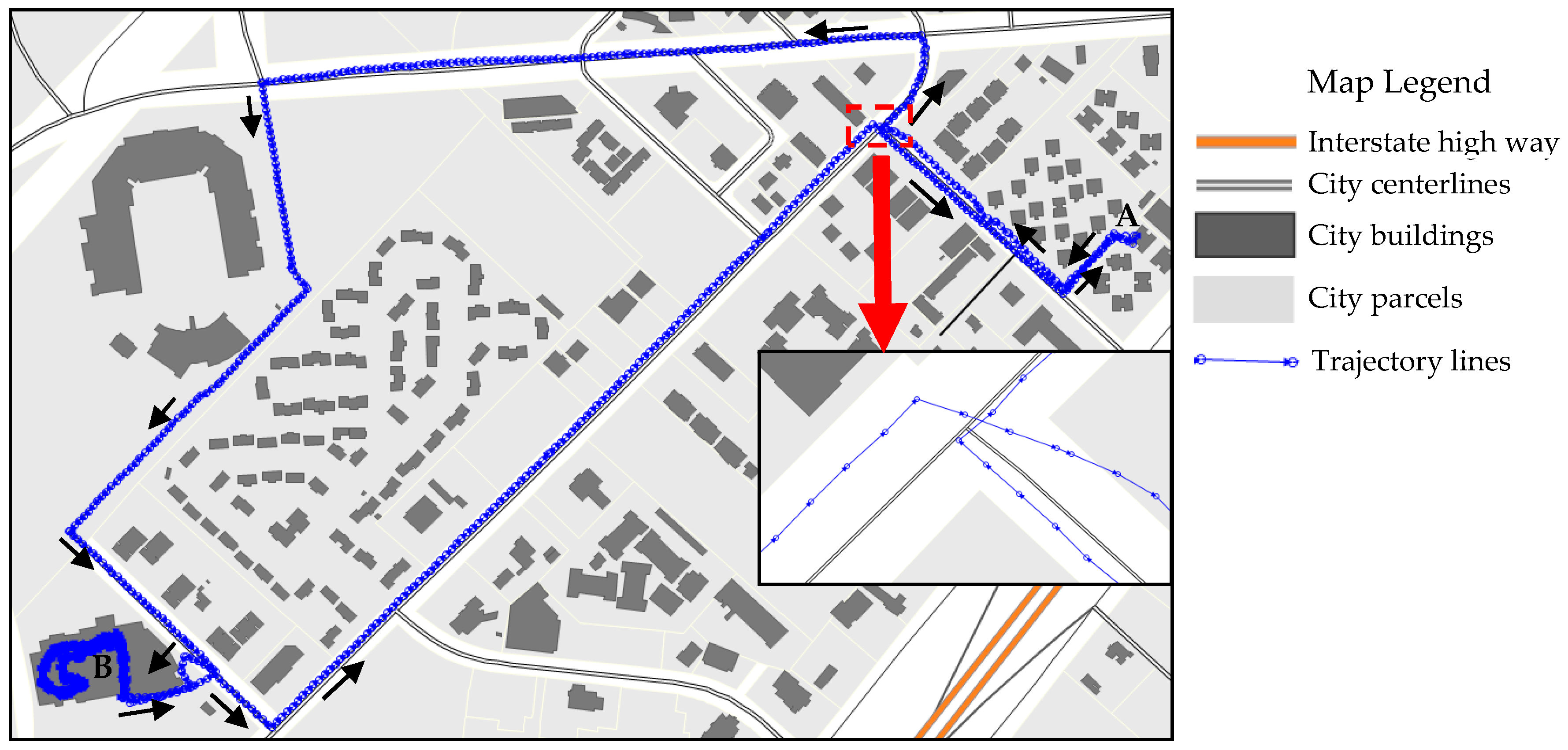
A GPS trajectory of 2010 points with mixed transportation modes. The subject began the trip from point A, walked to point B, and then took a bus traveling along the route of B→D→C→D→E→ F→G→H→I→J→K. The subject got off the bus at point K, walked to point L and back to K, and then took bus along the route of K→M→I→N→G→O→B. The subject got off the bus at point B and walked back to point A. The enlarged window shows the bus station at point B and the nearby GPS trajectory points.
Figure 6.
A GPS trajectory of 2010 points with mixed transportation modes. The subject began the trip from point A, walked to point B, and then took a bus traveling along the route of B→D→C→D→E→ F→G→H→I→J→K. The subject got off the bus at point K, walked to point L and back to K, and then took bus along the route of K→M→I→N→G→O→B. The subject got off the bus at point B and walked back to point A. The enlarged window shows the bus station at point B and the nearby GPS trajectory points.
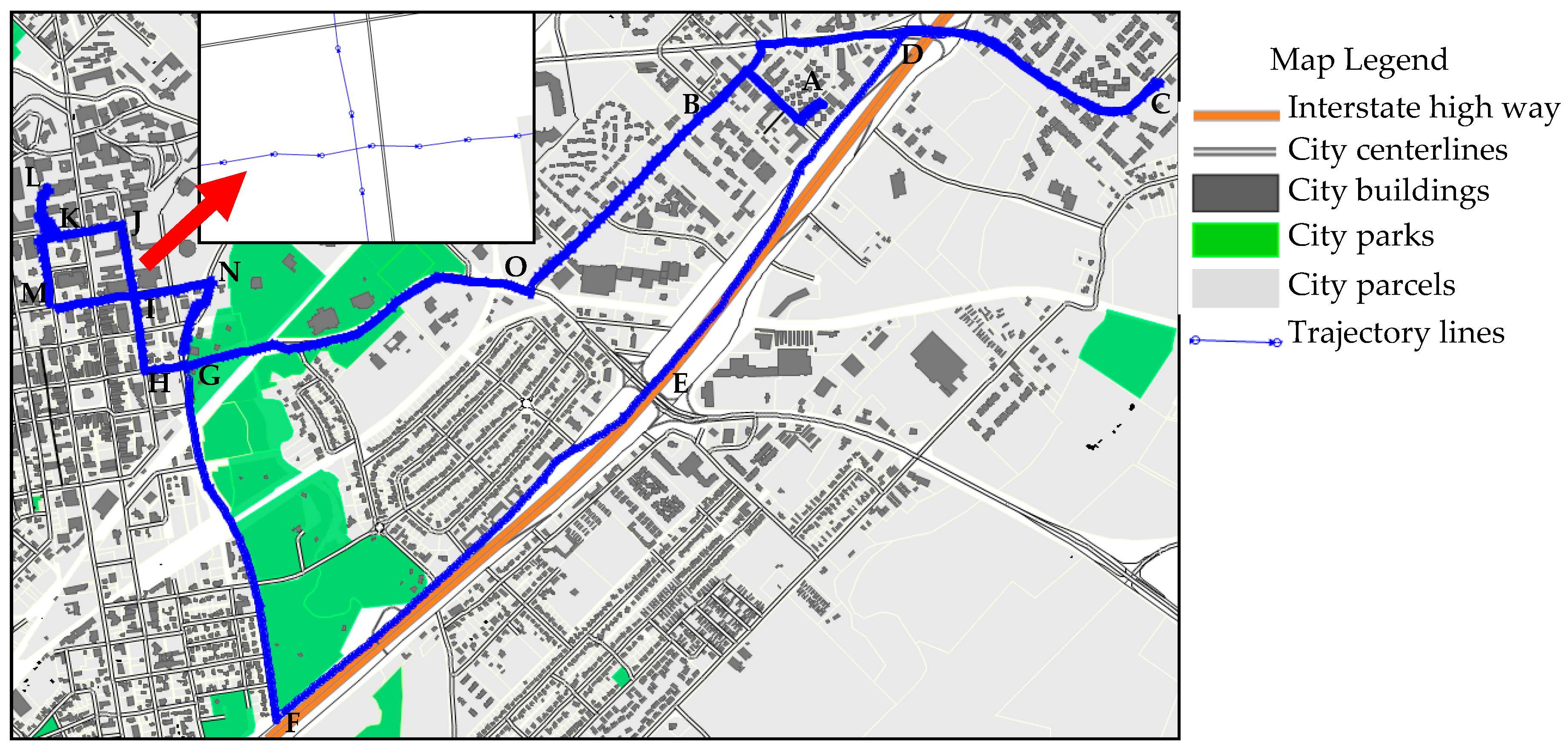
Figure 7.
Speed–time graph for: Trajectory 1 (a); and Trajectory 2 (b).
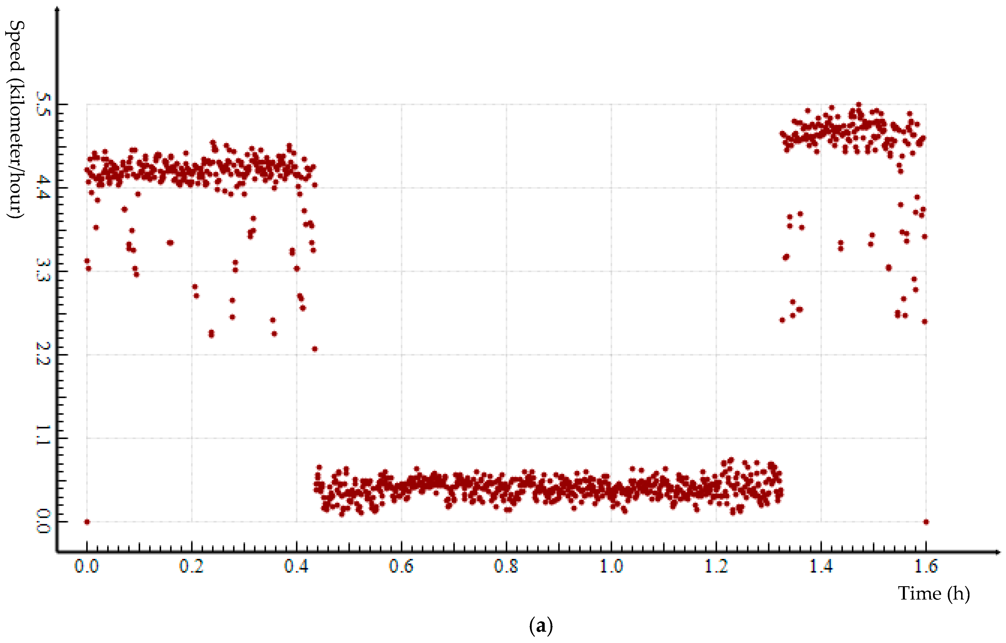

Figure 8.
Critical points identified by applying ESTC to the GPS data of Trajectory 1.
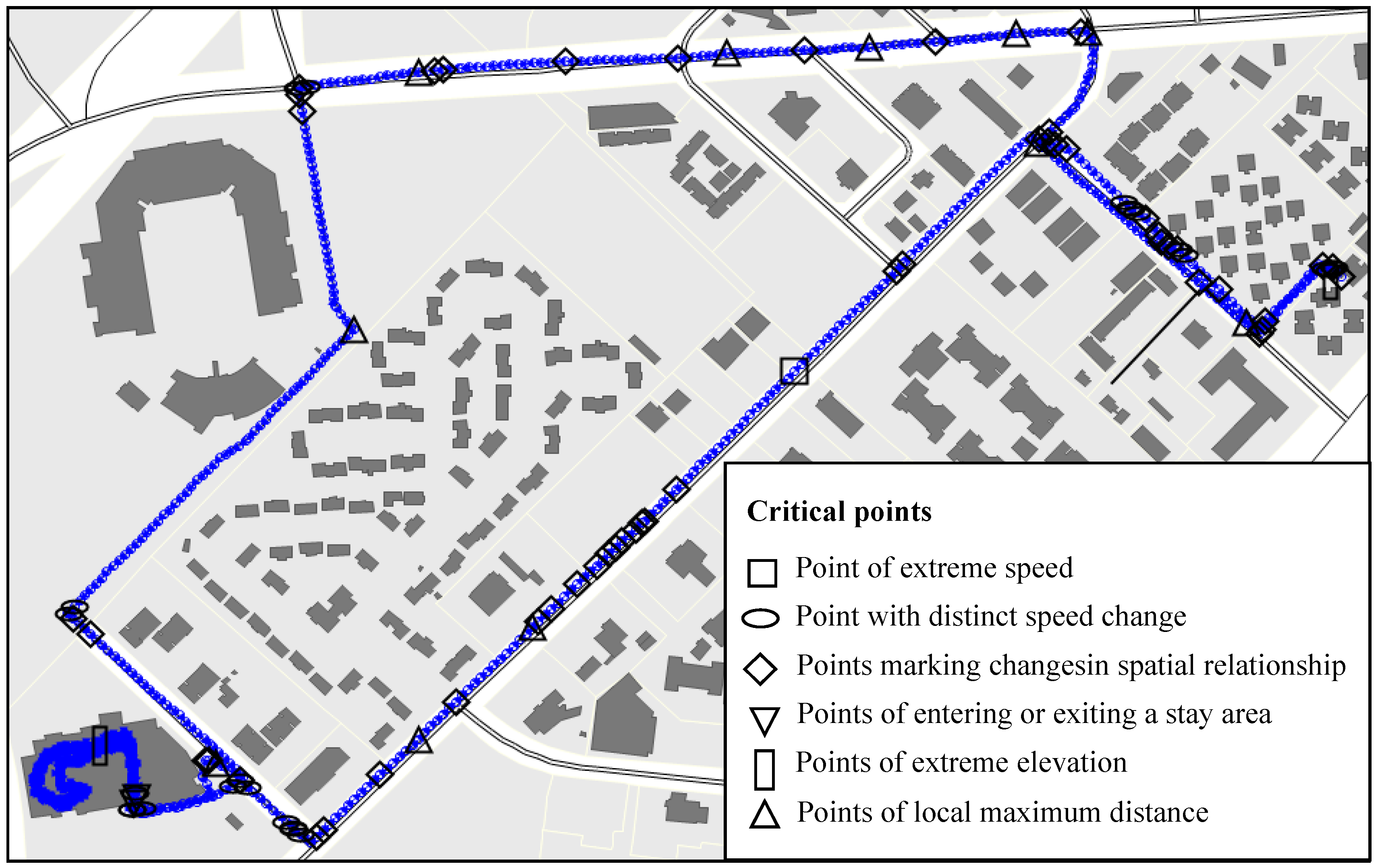
Figure 9.
Speed–time graphs of the original Trajectory 1 data and the simplified trajectory data based on DP and EDP algorithms with a distance threshold of: 1-m (a); 5-m (b); 10-m (c); and 25-m (d).
Figure 9.
Speed–time graphs of the original Trajectory 1 data and the simplified trajectory data based on DP and EDP algorithms with a distance threshold of: 1-m (a); 5-m (b); 10-m (c); and 25-m (d).
Figure 10.
Speed loss in the post-simplification data of Trajectory 1 using DP and EDP algorithms with a distance threshold of: 1-m (a); 5-m (b); 10-m (c); and 25-m (d).
Figure 10.
Speed loss in the post-simplification data of Trajectory 1 using DP and EDP algorithms with a distance threshold of: 1-m (a); 5-m (b); 10-m (c); and 25-m (d).

Figure 11.
Speed–time graphs of the original Trajectory 2 data the simplified trajectory data based on DP and EDP algorithms with a distance threshold of: 1-m (a); 5-m (b); 10-m (c); and 25-m (d).
Figure 11.
Speed–time graphs of the original Trajectory 2 data the simplified trajectory data based on DP and EDP algorithms with a distance threshold of: 1-m (a); 5-m (b); 10-m (c); and 25-m (d).


Figure 12.
Speed loss in the post-simplification data of Trajectory 2 using DP and EDP algorithms with a distance threshold of: 1-m (a); 5-m (b); 10-m (c); and 25-m (d).
Figure 12.
Speed loss in the post-simplification data of Trajectory 2 using DP and EDP algorithms with a distance threshold of: 1-m (a); 5-m (b); 10-m (c); and 25-m (d).
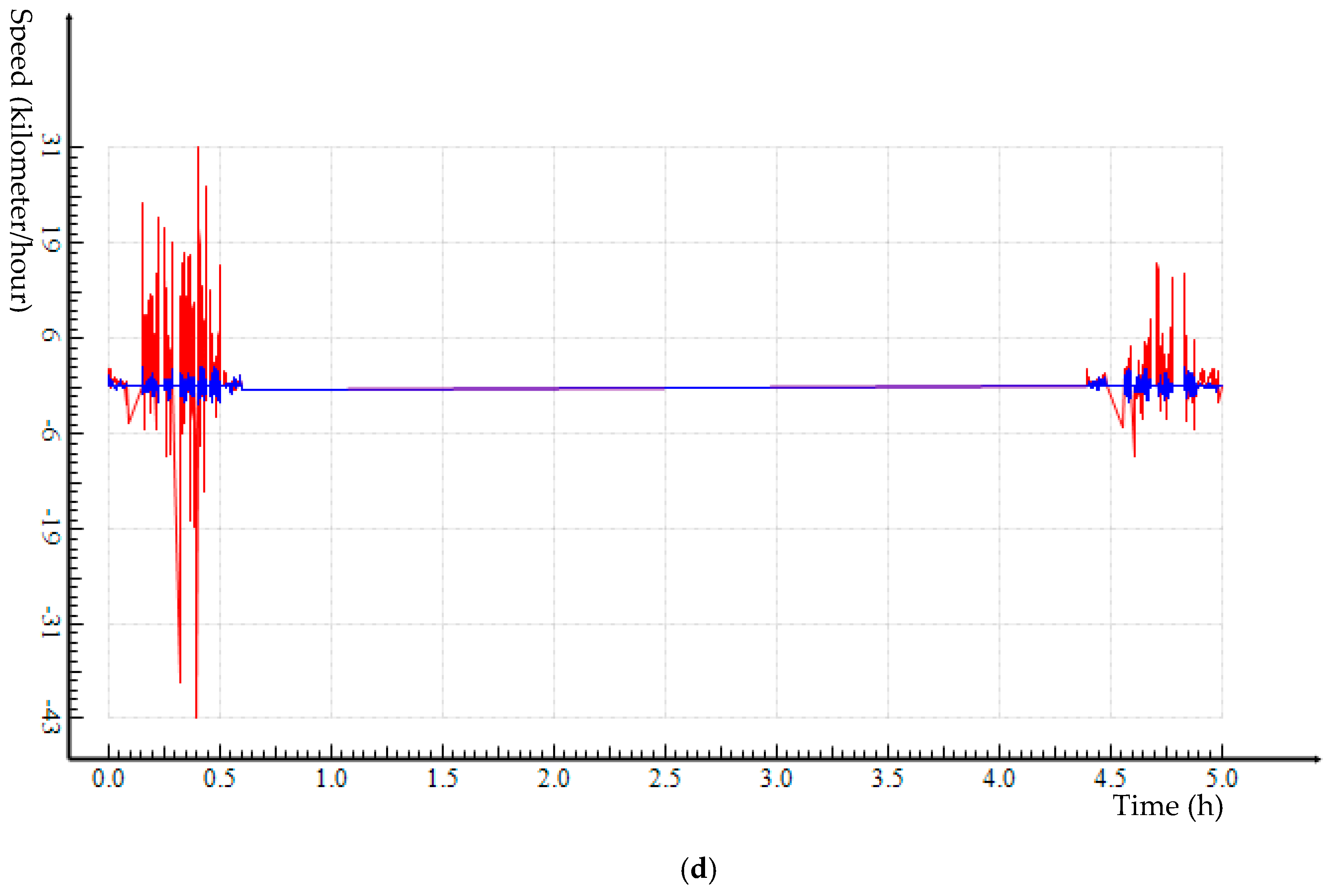
Figure 13.
Relative average speed loss and compression ratio of DP and EDP algorithms in the post-simplification data of Trajectory 1 with different distance thresholds.
Figure 13.
Relative average speed loss and compression ratio of DP and EDP algorithms in the post-simplification data of Trajectory 1 with different distance thresholds.

Figure 14.
Relative average speed loss and compression ratio of DP and EDP algorithms in the post-simplification data of Trajectory 2 with different distance thresholds.
Figure 14.
Relative average speed loss and compression ratio of DP and EDP algorithms in the post-simplification data of Trajectory 2 with different distance thresholds.

Table 1.
Points and critical points preserved by DP and EDP algorithms for Trajectory 1.
| Distance Threshold (m) | DP | EDP | Number of Critical Points Deleted by DP Incorrectly | ||
|---|---|---|---|---|---|
| Points Remained | Compression Ratio (%) | Points Remained | Compression Ratio (%) | ||
| 1 | 825 | 27.7 | 844 | 26.03 | 19 |
| 2 | 534 | 53.2 | 567 | 50.31 | 33 |
| 3 | 369 | 67.66 | 416 | 63.54 | 47 |
| 4 | 280 | 75.46 | 332 | 70.9 | 52 |
| 5 | 213 | 81.33 | 275 | 75.9 | 62 |
| 6 | 178 | 84.4 | 241 | 78.88 | 63 |
| 10 | 96 | 91.59 | 168 | 85.28 | 72 |
| 25 | 52 | 95.44 | 127 | 88.87 | 75 |
| 50 | 36 | 96.84 | 115 | 89.92 | 79 |
| 100 | 28 | 97.55 | 108 | 90.53 | 80 |
Table 2.
Speed loss of DP and EDP simplification on Dataset 1 with different distance thresholds.
| Distance Threshold (m) | DP | EDP Speed Loss (km/h) | ||||
|---|---|---|---|---|---|---|
| Total Speed Loss (km/h) | Average Speed Loss (km/h) | Relative Average Speed Loss (%) | Total Speed Loss (km/h) | Average Speed Loss (km/h) | Relative Average Speed Loss (%) | |
| 1 | 48.12 | 0.042 | 1.84 | 38.45 | 0.034 | 1.47 |
| 5 | 251.46 | 0.22 | 9.63 | 153.13 | 0.134 | 5.86 |
| 10 | 421.9 5 | 0.37 | 16.15 | 230.66 | 0.202 | 8.83 |
| 25 | 614.14 | 0.538 | 23.51 | 321.73 | 0.282 | 12.32 |
| 50 | 683.88 | 0.599 | 26.18 | 325.38 | 0.285 | 12.46 |
| 100 | 765.45 | 0.671 | 29.3 | 314.46 | 0.276 | 12.04 |
Table 3.
Points and critical points preserved by DP and EDP algorithms for Trajectory 2.
| Distance Threshold (m) | DP | EDP | Number of Critical Points Deleted by DP Incorrectly | ||
|---|---|---|---|---|---|
| Points Remained | Compression Ratio (%) | Points Remained | Compression Ratio (%) | ||
| 1 | 1441 | 28.31 | 1582 | 21.29 | 141 |
| 2 | 1053 | 47.61 | 1270 | 36.82 | 217 |
| 3 | 742 | 63.08 | 1050 | 47.76 | 308 |
| 4 | 559 | 72.19 | 908 | 54.83 | 349 |
| 5 | 446 | 77.81 | 828 | 58.81 | 382 |
| 10 | 203 | 89.90 | 642 | 68.06 | 439 |
| 25 | 130 | 93.53 | 602 | 70.05 | 472 |
| 50 | 95 | 95.27 | 592 | 70.55 | 497 |
| 100 | 67 | 96.67 | 582 | 71.04 | 515 |
Table 4.
Speed loss of DP and EDP simplification on Dataset 2 with different distance thresholds.
| Distance Threshold (m) | DP | EDP | ||||
|---|---|---|---|---|---|---|
| Total Speed Loss (km/h) | Average Speed Loss (km/h) | Relative Average Speed Loss (%) | Total Speed Loss (km/h) | Average Speed Loss (km/h) | Relative Average Speed Loss (%) | |
| 1 | 655.38 | 0.326 | 1.69 | 199.65 | 0.099 | 0.51 |
| 5 | 3241.85 | 1.612 | 8.35 | 632.1 | 0.314 | 1.63 |
| 10 | 5984.35 | 2.977 | 15.41 | 798.28 | 0.397 | 2.06 |
| 25 | 8306.99 | 4.133 | 21.39 | 840.3 | 0.418 | 2.16 |
| 50 | 9252.55 | 4.603 | 23.83 | 834.96 | 0.415 | 2.15 |
| 100 | 10305.14 | 5.127 | 26.54 | 840.78 | 0.418 | 2.17 |
© 2017 by the authors. Licensee MDPI, Basel, Switzerland. This article is an open access article distributed under the terms and conditions of the Creative Commons Attribution (CC BY) license (http://creativecommons.org/licenses/by/4.0/).
Share and Cite
MDPI and ACS Style
Qian, H.; Lu, Y. Simplifying GPS Trajectory Data with Enhanced Spatial-Temporal Constraints. ISPRS Int. J. Geo-Inf. 2017, 6, 329. https://doi.org/10.3390/ijgi6110329
AMA Style
Qian H, Lu Y. Simplifying GPS Trajectory Data with Enhanced Spatial-Temporal Constraints. ISPRS International Journal of Geo-Information. 2017; 6(11):329. https://doi.org/10.3390/ijgi6110329
Chicago/Turabian StyleQian, Haizhong, and Yongmei Lu. 2017. "Simplifying GPS Trajectory Data with Enhanced Spatial-Temporal Constraints" ISPRS International Journal of Geo-Information 6, no. 11: 329. https://doi.org/10.3390/ijgi6110329
Note that from the first issue of 2016, this journal uses article numbers instead of page numbers. See further details here.