Aircraft Reconstruction in High-Resolution SAR Images Using Deep Shape Prior

1
Institute of Electronic, Chinese Academy of Sciences, Beijing 100190, China
2
University of Chinese Academy of Sciences, Beijing 100190, China
*
Author to whom correspondence should be addressed.
ISPRS Int. J. Geo-Inf. 2017, 6(11), 330; https://doi.org/10.3390/ijgi6110330
Submission received: 8 September 2017
/
Revised: 9 October 2017
/
Accepted: 24 October 2017
/
Published: 31 October 2017
Abstract
:Contour shapes are important features. An accurate contour shape of a target can provide important prior information for applications, such as target recognition, which can improve the accuracy of target interpretation. In this paper, a synthetic aperture radar (SAR) target reconstruction method is proposed, which can be used to reconstruct the target by using shape priors to perform an accurate extraction of the contour shape feature. The method is divided into two stages. In the deep shape prior extraction stage, a generative deep learning modelling method is used to obtain deep shape priors. In the reconstruction stage, a novel coarse-to-fine pose estimation method combined with an optimization algorithm is proposed, which integrates deep shape priors into the process of reconstruction. Specifically, to address the issue of object rotation, candidate poses are obtained using the coarse pose estimation method, which avoids an exhaustive search of each pose. In addition, an energy function composed of a scattering term and shape term to combine the fine pose estimation, is constructed and optimized via an iterative optimization algorithm to achieve the goal of object reconstruction. To the best of our knowledge, this is the first time shape priors have been used to extract shape features of SAR targets. Experiments are conducted on a data set acquired by TerraSAR-X images and the results demonstrate the high accuracy and robustness of the proposed method.
1. Introduction
Object reconstruction is one of the primary tasks in the field of remote sensing image interpretation. It can obtain useful features with respect to objects, such as the shape and the size, and can thereby improve the accuracy and efficiency of target interpretation. However, according to the special imaging mechanism, geometric features such as double-bounce, layover and multi-bounce, and scattering centre features are the main features of synthetic aperture radar (SAR) images. Objects in SAR images are composed of a series of strong scattering points and are different from objects in natural or optical images. Therefore, it is difficult to utilize features such as texture, etc., for computer-assisted object reconstruction in SAR images.
In low-resolution SAR images, as shown in Figure 1a, strong scattering points are apparently independent and are clearly affected by azimuth, incident angle, and other imaging conditions. However, in high-resolution SAR images, many parts of the target generate strong scattering points, which makes the target more obvious and reduces effects on appearance. Therefore, the contour shape of the target is relatively stable under different imaging angles, as shown in Figure 1b. Traditionally, the contour shape feature can be extracted by computer vision method, such as the graph cut method [1], Chan-Vese segmentation method [2], the shape-based global minimization active contour model (SGACM) method [3] and so on.
However, taking the aircraft as an example, scattered information of oil patches on the ground as well as maintenance vehicles or loading vehicles near the gate position will be taken as parts of the aircraft. Moreover, the scattered information generated from some parts of the aircraft, such as smooth areas of the fuselage and plane areas of wings, is not obvious, which brings about partial deletion. Under the influence of the noise and the partial deletion mentioned above, the shape feature cannot be directly and easily obtained, thus it is difficult to perform accurate object interpretation, such as object detection and recognition. Therefore, accurate extraction of the contour shape feature becomes one of the key steps to achieve accurate object interpretation results in SAR images.
For human beings, the interpretation of an object in SAR images is usually conducted by the prior knowledge. For example, based on the regularities of distribution of strong scattering points, the shape, the size and the other information of the object can be judged according to existing prior knowledge. Then, the type of the object can be recognized in accordance with this information. Therefore, it is crucial to use known prior information for computer-assisted SAR image interpretation.
In previous studies, the prior information used by the researchers mainly included the distribution of strong scattering points, the intensity of scattered points, and the shape of object information, etc. Chen et al. [4] put forward a method of SAR object recognition based on key point detection and a feature matching strategy. Chang et al. [5] and Tang et al. [6] proposed a SAR object recognition method by means of SAR image simulation and scatter information research. Although these methods can achieve certain results, the information of scattering points in SAR images often changes with the imaging conditions, and it is difficult to obtain robust results only by using only the scattering point information. Zhang et al. [7] proposed a top-down SAR image building reconstruction method. This method succeeded in integrating priors of roof shapes into the object reconstruction model and achieving successful results. In SAR images, most of the strong scattering points can be used to reconstruct the shape of the object. By using shape priors, the robustness of object interpretation can be greatly improved as compared with methods only using the scattering point information.
However, how to express the prior knowledge as a reasonable mathematical expression is a difficult problem. Simple shapes, such as building roofs, can be represented with simple mathematical models. However, it is difficult to model shape priors for objects with complex shapes, such as aircrafts. To address the above issue, this paper presents a novel method of aircraft reconstruction in SAR images based on deep shape prior modelling. Innovations and contributions of this paper are summarized as follows:
Firstly, the shape prior is used in SAR aircraft reconstruction. In addition, to address the issue of modelling such complex shapes for aircrafts, we propose training a generative deep Boltzmann machine (DBM) [8] to model global and local structures of shapes as well as shape variations. After training a DBM, deep shape priors are represented by parameters of the DBM, which will be integrated into the underlying energy function to finally achieve the goal of object reconstruction.
Secondly, objects in SAR images are usually found in different poses, which is an obstacle when performing reconstruction. Without processing, the pose solution space is [0, 360). Since searching within the wide pose solution space is time consuming and the result easily trapped into local solutions, leading to low efficiency and accuracy, a pose estimation scheme is proposed which combines a novel coarse pose estimation method and a fine local pose estimation technique in the reconstruction stage. Specifically, the former coarse pose estimation method contains two main steps. In the symmetric transform step, the image is translated to a symmetric form and the pose of the object will be estimated within eight certain poses via using the transform invariant low-rank textures (TILT) method in Zhang et al. [9] to avoid an exhaustive search in the space [0, 360). In the symmetric detection step, a correlation analysis method is conducted to detect the symmetric type and then obtain two candidate poses, which will be used when performing object reconstruction. Moreover, the latter fine local pose estimation technique is integrated into the optimization of the energy function and is detailed in Algorithm 1. In general, the proposed pose estimation scheme can significantly improve the efficiency and the accuracy of object reconstruction.
Thirdly, to address the issue of integrating deep shape priors into the aircraft reconstruction stage, an energy function is defined by integrating a scattering term and a shape term, among which the deep shape prior corresponds to the shape term. Moreover, scattering points and their edge information of the transformed image after coarse pose estimation form the scattering term. Finally, an improved iterative optimization method based on the split Bregman algorithm [10] is introduced to minimize the energy function. To the best of our knowledge, this is the first attempt at reconstructing complex objects and extract information in SAR images using shape priors.
To verify the effectiveness of the proposed method, we have carried out experiments on a TerraSAR-X data set with a resolution of 0.5 m and 1.0 m. Experimental results show that the proposed method can reconstruct the object more robustly. In addition, we compare the proposed method with conventional methods based on contour segmentation. The results show that the use of deep shape priors can assist the object reconstruction, which greatly improves the accuracy of object reconstruction.
2. Data Description and Analysis
2.1. Data Description
In this paper, test slices are collected from TerraSAR-X Spotlight-0.5 m (ST) and ST-1.0 m modes high-resolution images. However, values 0.5 and 1.0 are not exact resolution values. For example, Table 1 shows the mode and the corresponding resolution of two images. As shown in this figure, azimuth and range resolutions are not equal to each other and both have mode values 0.5 and 1.0, respectively. Therefore, for convenience, mode values are used instead of exact resolutions, and are 0.5 m and 1.0 m.
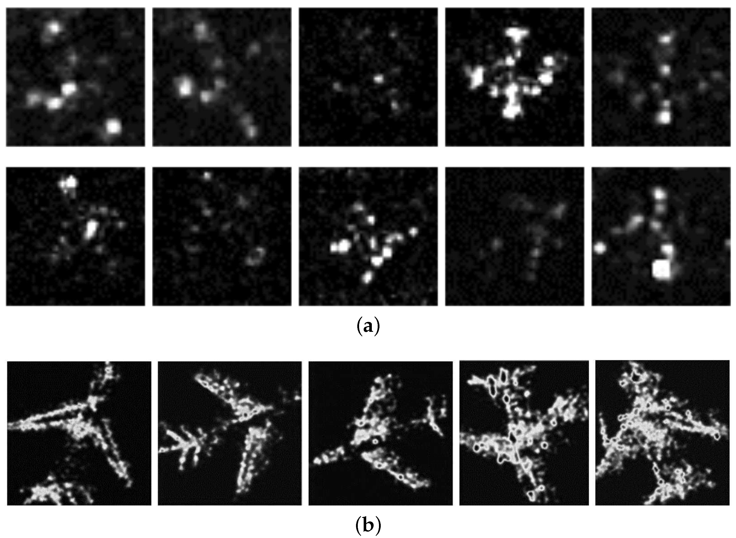
At the airport, aircrafts are parked in variant orientations. Figure 2 shows examples of image slices with resolution of 1.0 m and 0.5 m. They are used as a validation data set. The figure reveals that TerraSAR-X images with a resolution of 1.0 m or a higher resolution of 0.5 m have abundant information. Specifically, the head, wings and tails of the aircraft are relatively distinguishable. This is the basis of accurate aircraft reconstruction. Nevertheless, scattering features in regions of the body, wings and tails have vanished bringing challenges for traditional reconstruction methods without shape priors and requiring integration of shape priors into object reconstruction so as to obtain the full contour information of objects.
In the last section of this paper, to evaluate the reconstruction results quantitatively, the percentage of misclassified pixels (PMP) [11] is used as the evaluation criterion of the reconstruction accuracy. In Function (13), and represent background and foreground pixels of ground truth, respectively. In general, the ground truths are labelled manually. Firstly, the type, the location and the angle of the object in each validation data slice are labelled by the experience of experts, or by comparing optical and SAR images in the same region and the same time. Specifically, the experience of experts is divided into two types. The first type is experience a priori within a particular region including types and locations of all aircrafts that are parked within this region. The second is experience with respect to the characteristic of SAR objects, which can help to distinguish the type and the location of the aircraft in SAR images. Secondly, according to this information, the shape template of labelled type is transformed to obtain the ground truth. For example, Figure 3a is a validation data slice with labelled information, and Figure 3b is the transformed shape template, which is the ground truth of the data slice in Figure 3a.
2.2. Shape Prior Description
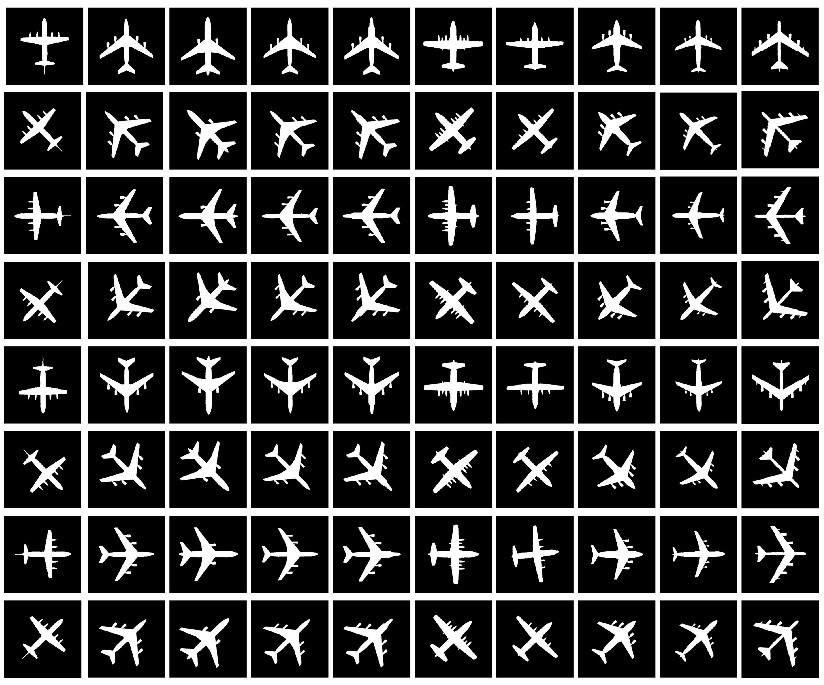
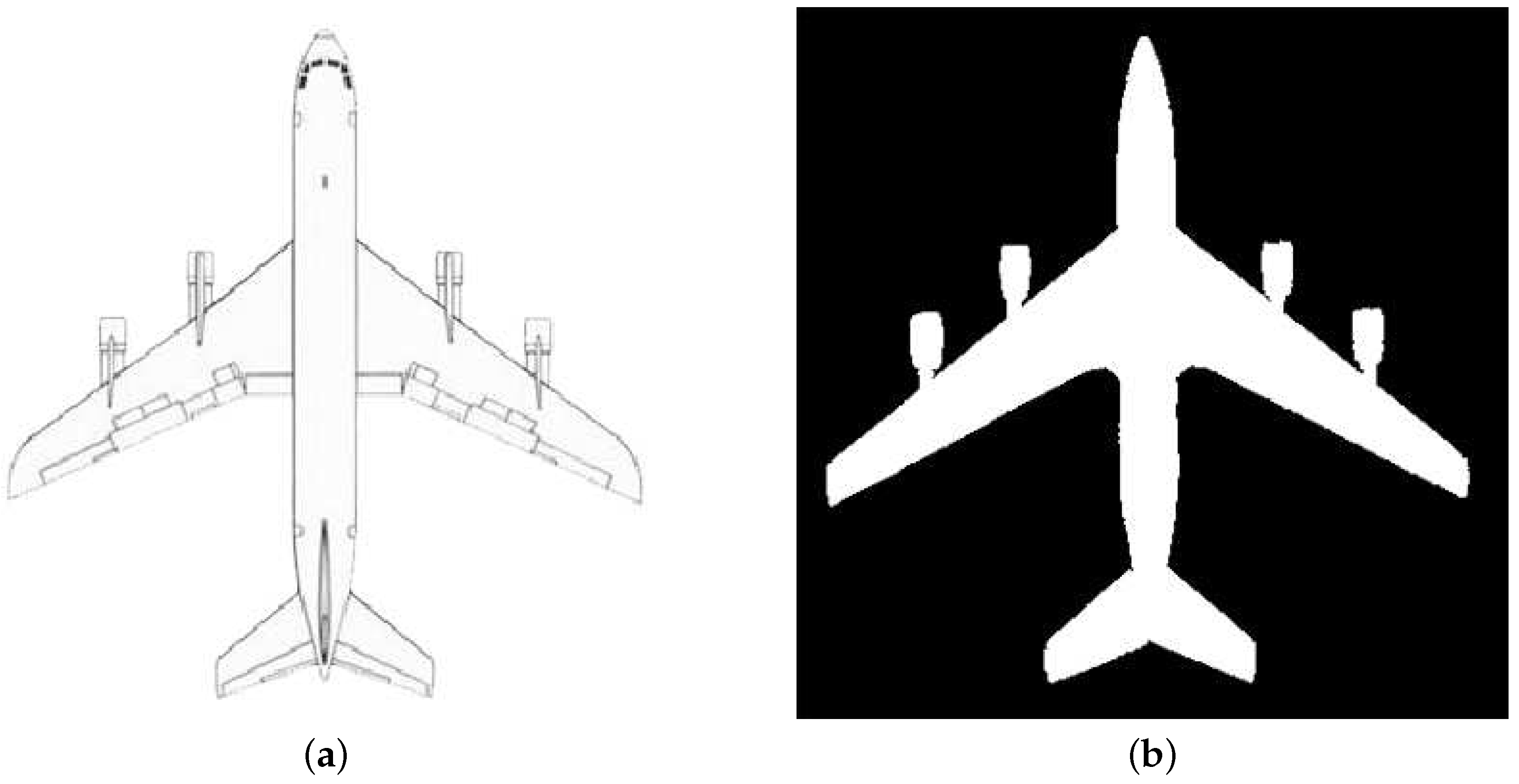
In this paper, shape templates are represented by binary images in Figure 4, including eight sets of binary shape images at 0, 315, 270, 180, 135, 90 and 45 degrees. Among them, each binary shape is the contour of a top-view drawing for a certain type of aircraft, with pixel values of the inner of the aircraft contour being filled with 255 and the outer of the aircraft contour being filled with 0, which can be seen in most of the shape prior-based method [3,12]. For example, Figure 5 shows the top-view drawing of an aircraft’s and the corresponding binary shape. In our experiments, shape templates include 10 types of aircrafts. They are a similar cross structure, and different lengths, widths and appearance of wings, engines and head shapes. The existence of these obvious similarities and differences in structures makes it efficient to model the shapes by using multi-layer neural networks.
In the proposed method, deep shape models are pre-trained for shape representation at each angle to obtain deep shape prior models. Then, after pose estimation, candidate poses are successively used to choose corresponding deep shape prior as the shape term for constructing the energy function.
3. Methods
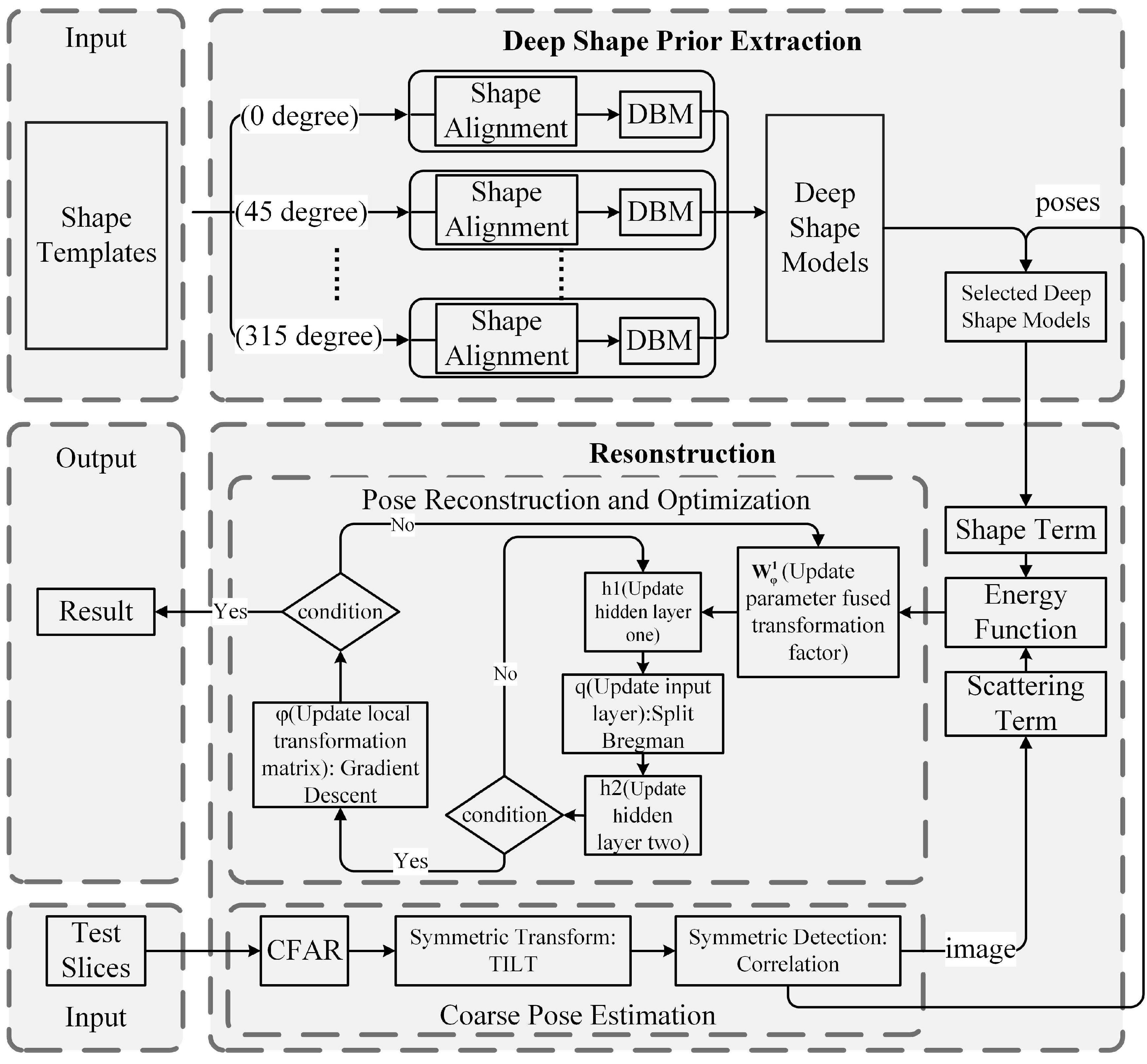
In this section, ideas of the proposed method as well as some implementation details will be described. As shown in Figure 6, the proposed method contains two main stages: the deep shape prior modelling stage and the reconstruction stage. Specifically, the shape models pre-trained in the first stage are used as shape constraints in the second stage. To realize efficient object reconstruction, a coarse pose estimation method is conducted at the beginning of the object reconstruction stage to obtain candidate poses and the processed symmetric image, which makes the proposed method fit for objects in different orientations. Then, the selected shape priors with local transformation parameters and the processed SAR image are used to form the energy function. Finally, an iterative optimization algorithm is carried out to minimize the energy function.
Notably, the input data sets are preprocessed by the constant false alarm rate (CFAR) [13] method to achieve background noise removal and improve the accuracy of coarse pose estimation and object reconstruction. More implementation details are summarized in the following subsections.
3.1. Deep Shape Prior Extraction
3.1.1. Shape Alignment
The shape is a typical feature for objects, which can characterize the distinctive structures of different objects or detailed structures of each object. Since generative deep learning models like DBM have the specific property of generating realistic samples, they can generate samples which are different from shapes in our training set [14]. Since the size of the shape is fixed according to the known resolution, we just need to perform the shape alignment. To this end, the method of Liu et al. [3] is used for the binary shape templates with the centre of gravity being aligned with formula defined as follows:
where is the centroid of the shape template, while the variable S denotes the pixel value of . Then, the scale alignment is defined as follows:
where and represent normalization parameters, which are used to scale each shape template. Figure 7 shows results of the shape alignment. As shown in this figure, shape templates are set to their center of gravity and are regularized to a certain scale, which can be translated to other scale with different resolution directly.
3.1.2. Shape Prior Models
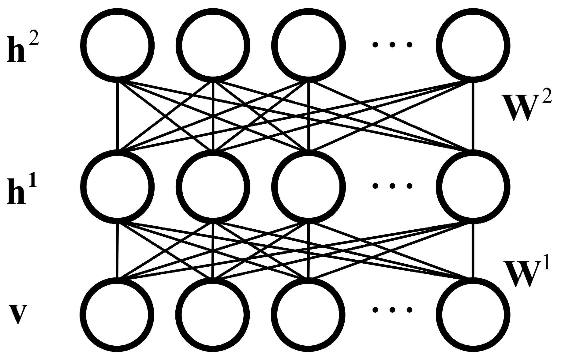
After the shape alignment, a three-layered DBM, which is shown in Figure 8, is used to model the shape priors by maximizing the distribution of the visible layer, which is denoted by . However, the calculation of is difficult. Therefore, approximate inference is used via an efficient Gibbs sampling, which is detailed in [8,12] and is shown in Figure 9. The energy function of the three-layered shape model is defined as:
where variables , and are the first hidden layer, the second hidden layer and the visible layer of DBM, respectively. Parameters in are DBM parameters, which can represent the deep shape prior, in which and are weight metrics between the visible layer and the first hidden layer, and the two hidden layers, respectively. , and are biases of the first hidden layer, the second hidden layer and the visible layer, respectively. Some of these variables and parameters are labelled in Figure 8.
After training the three-layered DBM, the processed image is imported to the network to obtain the shape image via the sampling process, which is shown in Figure 9. Activation functions used are defined as follows:
where is a sigmoid function. Variables listed above are also labelled in Figure 9, in which variables , , and are elements of the visible layer, the first hidden layer, and the second hidden layer of DBM, respectively. Parameters and are elements of and in Function (3). Parameters and and are elements of biases in the first hidden layer, the second hidden layer, and the visible layer, respectively.
In this paper, parameters are chosen as 100 for the first hidden layer and 300 for the second hidden layer with best performance. The parameter , which responds to the input image, is visualized in Figure 10 by a calculation function in [15]. The figure reveals that the cross structure is obvious, which characterizes typical aircraft characteristics.
Owing to the representation of local and global features, the deep shape prior obtained in the former subsection is stable to objects with absent parts, i.e., the second column in Figure 11a. As shown in Figure 11b, the deep shape prior is still complete, although the object has absent parts. In SAR images, due to the special imaging mechanism, some parts of the objects are absent as shown in Figure 2, which brings difficulties to object reconstruction. The deep shape prior can solve this challenge task via its insensitivity to components absence.
Up to this point, the DBM parameters , which are used as shape constraints in the reconstruction stage, can represent local and global features of shape templates.
3.2. Coarse Pose Estimation
Objects in SAR images can be in any pose, which makes deep shape prior extraction be a challenging task. To address this issue, the coarse pose estimation method is described in this subsection. Poses of objects will be constrained into two specific values by means of symmetric transformation and symmetric detection. In this case, zygomorphic, laterally zygomorphic, principal-diagonal symmetry and counter-diagonal symmetry are corresponding to poses of 0 and 180, 90 and 270, 135 and 315, 45 and 225 degrees. This means that one type of symmetry only represents two candidate poses.
In the symmetric transform step, an approximate symmetric image can be translated by the TILT algorithm to obtain image (i.e., X) with approximate symmetric appearance within the above four symmetric styles. By doing so, only eight poses can be confirmed to be candidate poses.
In the symmetric detection step, correlation coefficients of the image matrix are used to determine the kind of symmetry it is, which can be defined as:
where is the correlation coefficient of X and . S and D denote the symmetric type and the translation distance, respectively, while represents the translated image of X with a certain symmetric type and translation distance.
Finally, two candidate poses can be determined according to the maximum value of all correlation coefficients. At the same time, the object in the output image is translated according to parameter D. As shown in Figure 6, outputs of the coarse pose estimation (i.e., image and poses) are used to construct the energy function.
3.3. Pose Reconstruction and Optimization
After the coarse pose estimation and the deep shape prior extraction, an energy function is defined by the combination of the deep shape prior and the processed image. Here, a classical probabilistic shape representation method [12,16] is used as the basic function and is modified via combining the shape term and the scattering term, which is defined as follows:
where represent parameters of the shape prior model. Since researchers have confirmed that the localities and the intensities of strong scattering centres over a certain span of azimuth angles are statistically quasi-invariant [17], the weight is modified as , in which represents the local transformation matrix and is defined as follows:
among which are the locally transformation parameters, i.e., a translation of the first and second dimension, the scale, and the rotation angle, respectively.
For the scattering term, is the contour of the scattering region which is defined as
while distinguishes the scattering region and the background, which is defined as follows:
where and are the contour indicator and the gradient of the scattering region, respectively, with . is the image space. and are the mean intensity of the scattering region and the background region, which are defined as and , respectively. Inside, is the processed image and is the scattering region, which is with a selected threshold.
Reconstruction results are obtained by optimize the energy function with an iterative minimization procedure, in which the approximate inference of DBM [12] is introduced for the calculation of each layer of hidden units, and split Bregman, a traditional algorithm for convex optimization, is used to calculate the shape. Details of the optimization process are summarized in Algorithm 1, while Algorithm 2 is the details of Split Bregman method to solve the problem of minimizing in Algorithm 1 step 2.3.
As shown in Algorithm 1, parameters are initialized in advance. Since the resolution is a known number, the scale h is fixed. For objects that have already been transformed, x, y, and are set to be 0. Specifically, if the object in the slice is not centroid, x, y will be set to be values obtained by the symmetry axis in the coarse pose estimation. For example, if symmetry axis of the object in the slice is or , the initializations of x, y in Algorithm 1 for are set to be , or , . At the same time, the shape is set to be the mean shape of the templates while the hidden units are initialized by . Besides, the set of the learning rate in the gradient descent, which is used to update , is set to be small values for local adaption. The optimization will be continued until the energy difference is less than the threshold or the maximum number of iterations is reached.
After that, reconstruction results with candidate poses are obtained. The one with the minimum energy value is chosen as the final result.
| Algorithm 1 Optimization Algorithm |
| Input: Learned parameters fused by transformation factor , test image slice |
| Initialization: |
| Initialize as mean shape of the data set, set , , , , and maximum numbers of iteration , . |
| Optimization: |
| Repeat 1 to 3 until or the maximum number of iteration is reached. |
| 1. Calculate and let . |
| 2. Repeat 2.1 to 2.5 until or the maximum number of iteration is reached. |
| 2.1 |
| 2.2 |
| 2.3 |
| 2.4 |
| 2.5 Calculate by Function (9). |
| 3. Update using the gradient descent technique. |
| 3.1 Calculate using |
| 3.2 Calculate |
| Output: The latest shape . |
| Algorithm 2 Detailed steps in Algorithm 1 2.3 |
| Input: Parameters , , , . |
| Repeat 1 to 5 until or the maximum number of iterations is reached. |
| 1. Define: |
| 2. |
| 2.1 |
| 2.2 |
| 3. |
| 4. Find |
| 5. Renew |
| Output: The latest shape . |
3.4. Parameter Selection
In this subsection, parameters in Algorithm 1 and Algorithm 2 are described. In practice, these parameters are set mainly based on experience. In our experiments, the convergence parameter is set to . The maximum numbers of iterations , , and are set to be 10, 100, and 50, respectively. To achieve fine tuning, the learning rate of the transformation parameter is set to small numbers. In our experiment, it is set to be . In addition, parameters and are related to each other. Among them, represents the importance of the scattering edge term and is also the coefficient of the first part in Function (9) which is set to be 1.0 by defaults. The other two parameters are set according to . represents the importance of the scattering region term, while represents the importance of the deep shape term. In object reconstruction, the region term is the most important part. The shape term and the edge term are priors. In our experiments, and are set to be 100.0 and 1.0, respectively. In addition, represents the distinguished threshold of inner and outer object which is set to be 0.1 for SAR aircraft reconstruction.
4. Experimental Results and Analysis
In this section, we will describe the protocols to test the performance of the proposed reconstruction method. Experiments are organized into three parts. The first part shows the results of the coarse pose estimation. In the second part, the proposed method will be compared with segmentation based methods without shape priors. In the last part, the proposed method with deep shape priors is compared with traditional shape prior based method.
4.1. Coarse Pose Estimation
In this subsection, results of the proposed coarse pose estimation method are shown in Table 2 and Figure 12.
When performing the coarse pose estimation, the accuracy is low due to the background noise. In this paper, the CFAR detection technique is conducted to realize noise removal. The statistical model of background is modelled and can obtain the object region by setting a constant false alarm rate. Table 2 shows the results of the coarse pose estimation without image preprocessing and with image preprocessing using the traditional histogram threshold method and the CFAR detection technique. The experimental results show that the coarse pose estimation with image preprocessing based on the CFAR detection technique has a higher accuracy.
Figure 12a shows data slices of different types of aircrafts with different poses. After preprocessing by CFAR, the TILT method is used to transform objects in these slices to certain symmetric patterns. As shown in the first column of Figure 12b, the object is transformed to a zygomorphic form. Afterwards, the type of the symmetric pattern is detected in the symmetric detection step by image correlation. As shown in Figure 12b, symmetric patterns are all detected correctly as zygomorphic, counter-diagonal symmetric, zygomorphic, laterally zygomorphic, and laterally zygomorphic from left to right.
In general, each symmetric pattern corresponds to two fixed poses. For example, for the first slice in Figure 12b, the red line indicates the directions of zygomorphic symmetric pattern, which are 0 and 180. As such, the reconstruction procedure is simplified in latter steps, only two sets of deep shape priors at 0 and 180 degrees are chosen as shape terms of the energy function, from which the one with the most minimal energy value is the final result. Results in Table 2 and Table 3 demonstrate that the proposed coarse pose estimation method integrated into the reconstruction procedure can address the issue of object rotation.
4.2. Aircraft Reconstruction
To evaluate reconstruction results quantitatively, we use the percentage of misclassified pixels (PMP) [11] for the measurement of the reconstruction accuracy, which is defined as follows:
where ⋂ and denote the intersection of two regions and the number of pixels of inner region, respectively. and represent background and foreground pixels of the ground truth, respectively. Meanwhile, and are the background and foreground pixels of the reconstruction result, respectively. In general, the lower the value of PMP is, the better the reconstruction result will be.
To validate the effectiveness of the proposed method, the typical segmentation-based methods graph cut [1], Chan-Vese segmentation [2] and SGACM [3], as well as our method without shape priors are chosen for comparison. The reconstruction accuracies of these methods are listed in Table 3.
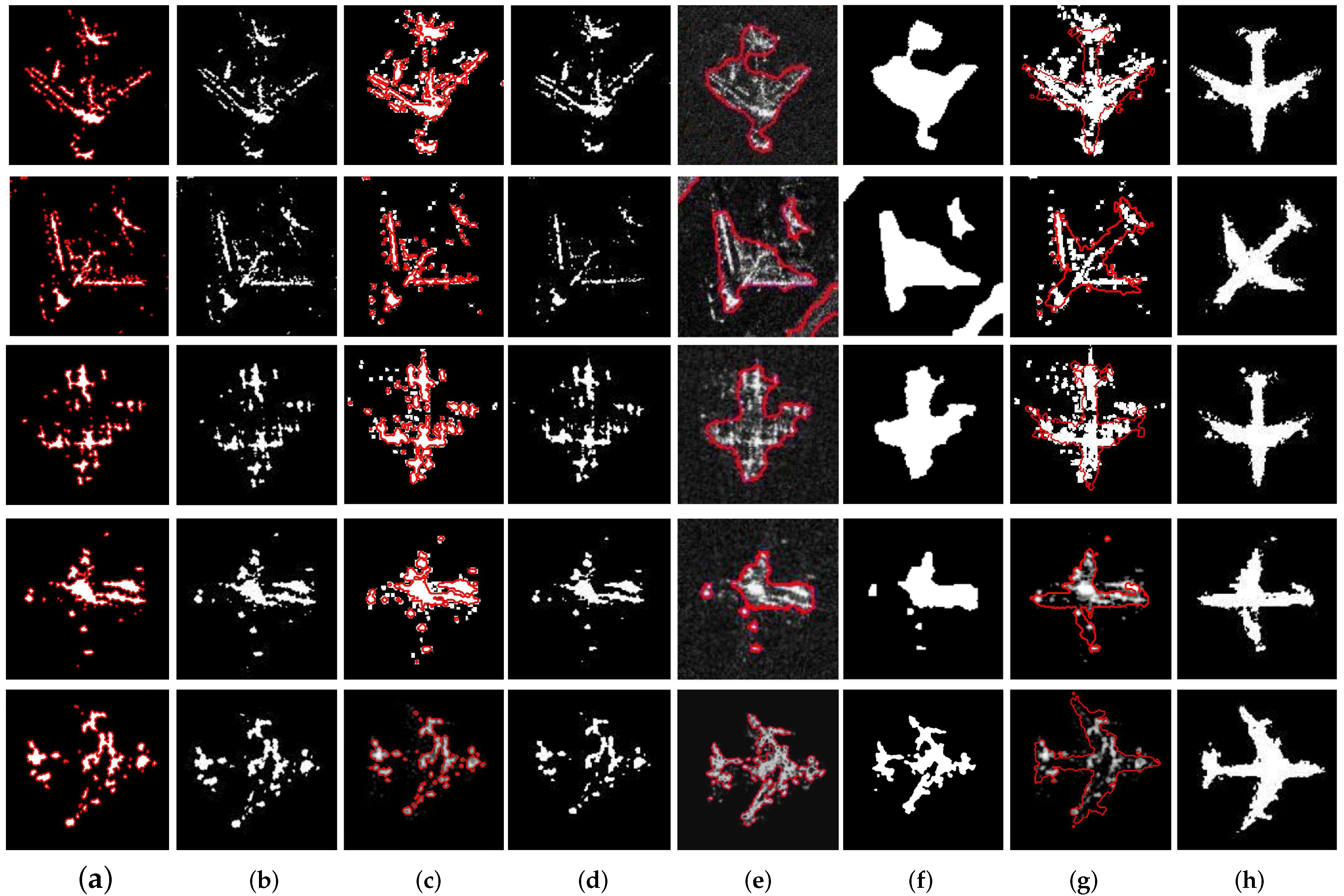
Moreover, graphical reconstruction results are shown in Figure 13, among which the white regions are the reconstructed object regions and the red lines in Figure 13a,c,e,g are shape contours of the reconstructed objects. These results show that the proposed method is the most efficient method, with the highest reconstruction accuracy.
4.2.1. Shape Prior
By analysis of PMPs in Table 3, we found that shape prior-based methods, i.e., SGACM and the proposed method, have approximatly 20–30% lower PMP values than the graph cut method and have 10–20% lower PMP values than the Chan-Vese Segmentation method, which demonstrates that the use of shape priors can improve reconstruction accuracy.
As shown in Figure 13, the contour of the object and the reconstructed object region are visualized. It should be noted that the results of the graph cut method and the Chan-Vese segmentation method are rotated artificially for the comparison between methods. In Figure 13a,b, the segmentation-based graph cut method has difficulties in integrating the scattering points of the object into SAR image. In addition, if the shape prior is not applied, with visualization in Figure 13c,d, the proposed method will obtain similar results to the graph cut method. Similarly, in Figure 13e,f, the Chan-Vese segmentation method has difficulties in reconstructing the absent parts of the object in the data slice, which results in relatively poor reconstruction accuracy. In contrast, the proposed method with shape priors can reconstruct comparatively complete object contours and obtain whole object region with a high accuracy. Thus, the analysis of experimental results demonstrate that shape priors can significantly improve the accuracy of object reconstruction.
4.2.2. Deep Shape Priors
In the previous subsection, experiments were conducted to validate the effectiveness of integrating the shape prior into object reconstruction. In this subsection, the deep shape priors used in this paper are compared with traditional shape priors in SGACM to validate the effectiveness of deep shape priors.
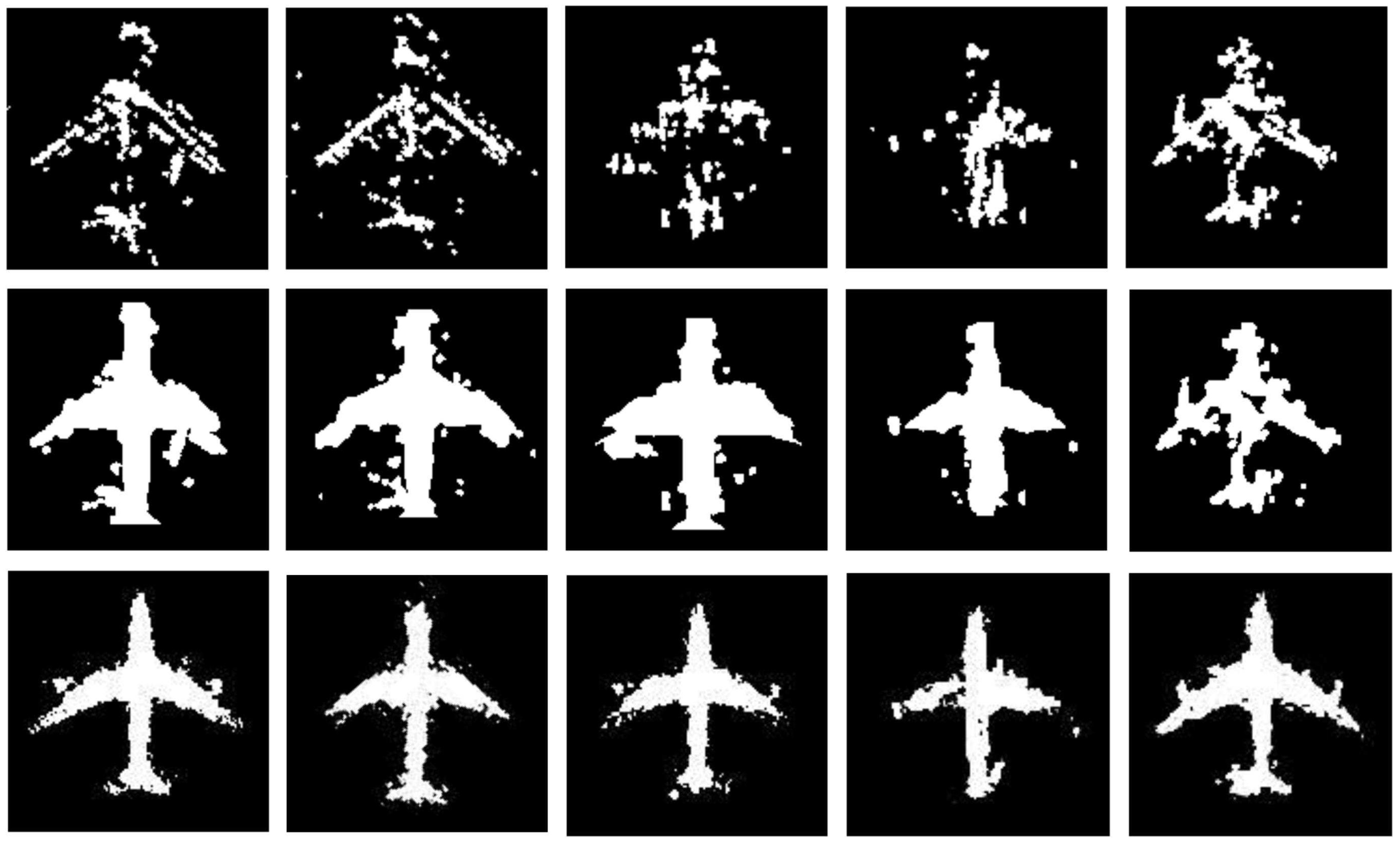
Firstly, it should be emphasized that the SGACM method cannot handle the issue of object rotation. As a result, objects are turned into the same pose manually before using the SGACM method, which is shown in Figure 14. To compare with these two methods, coarse pose estimation is replaced by manual rotation. According to results in Table 3 and Figure 14, although SGACM method also utilizes shape priors, the deep shape prior is more robust. Moreover, as we can see in Figure 12, due to the effectiveness of the coarse pose estimation, the proposed method can be applied to objects at different poses automatically, which addresses the issue of object rotation in SAR images.
In conclusion, the proposed method can effectively reconstruct aircrafts in high-resolution SAR images at any angle.
5. Conclusions
In this paper, we have proposed a novel method to address the issue of aircraft reconstruction in high-resolution SAR images. The method is mainly divided into two stages: the deep shape prior extraction stage and the object reconstruction stage. In the former stage, a generative deep network, DBM, is used to pre-train deep shape priors, while, In the latter stage, a novel two-step framework is proposed to integrate deep shape priors into object reconstruction. Specifically, pose estimation is conducted by symmetric characteristics to address the issue of object rotation. After that, the constructed energy function is minimized by an iterative optimization method based on approximate inference and split Bregman to achieve reconstruction results. Experimental results show that the proposed method can reconstruct objects with high accuracy and can obtain the pose of the object simultaneously, which provides benefits with respect to further applications, e.g., object detection and recognition.
Our future work may focus on the extension of the proposed method to other interesting objects and the end-to-end framework for object reconstruction.
Author Contributions
Fangzheng Dou, Wenhui Diao and Kun Fu conceived and designed the experiments; Fangzheng Dou and Wenhui Diao performed the experiments; Fangzheng Dou, Xian Sun and Yue Zhang analyzed the data; Fangzheng Dou wrote the paper.
Conflicts of Interest
The authors declare no conflict of interest.
References
- Boykov, Y.Y.; Jolly, M.P. Interactive graph cuts for optimal boundary & region segmentation of objects in N-D images. In Proceedings of the Eighth IEEE International Conference on Computer Vision, Vancouver, BC, Canada, 7–14 July 2001; pp. 105–112. [Google Scholar]
- Pascal, G. Chan-Vese Segmentation. Image Process. Line 2012, 2, 214–224. [Google Scholar]
- Liu, G.; Sun, X.; Fu, K.; Wang, H. Interactive geospatial object extraction in high resolution remote sensing images using shape-based global minimization active contour model. Pattern Recognit. Lett. 2013, 34, 1186–1195. [Google Scholar] [CrossRef]
- Chen, J.; Zhang, B.; Wang, C. Backscattering feature analysis and recognition of civilian aircraft in TerraSAR-X images. IEEE Geosci. Remote Sens. Lett. 2015, 12, 796–800. [Google Scholar] [CrossRef]
- Chang, Y.L.; Chiang, C.Y.; Chen, K.S. Sar image simulation with application to target recognition. Prog. Electromagn. Res. 2011, 119, 35–57. [Google Scholar] [CrossRef]
- Tang, K.; Sun, X.; Sun, H.; Wang, H. A geometrical-based simulator for target recognition in high-resolution sar images. IEEE Geosci. Remote Sens. Lett. 2012, 9, 958–962. [Google Scholar] [CrossRef]
- Zhang, Y.; Sun, X.; Thiele, A.; Hinz, S. Stochastic geometrical model and monte carlo optimization methods for building reconstruction from insar data. ISPRS J. Photogram. Remote Sens. 2015, 108, 49–61. [Google Scholar] [CrossRef]
- Salakhutdinov, R.; Hinton, G. Deep boltzmann machines. J. Mach. Learn. Res. 2009, 5, 1967–2006. [Google Scholar]
- Zhang, Z.; Liang, X.; Ganesh, A.; Ma, Y. Transform invariant low-rank textures. In Proceedings of the Asian Conference on Computer Vision, Queenstown, New Zealand, 8 November 2010; pp. 314–328. [Google Scholar]
- Goldstein, T.; Bresson, X.; Osher, S. Geometric applications of the split bregman method: Segmentation and surface reconstruction. J. Sci. Comput. 2010, 45, 272–293. [Google Scholar] [CrossRef]
- Wu, Q.; Diao, W.; Dou, F.; Sun, X.; Zheng, X.; Fu, K.; Zhao, F. Shape-based object extraction in high-resolution remote-sensing images using deep boltzmann machine. Int. J. Remote Sens. 2016, 37, 6012–6022. [Google Scholar] [CrossRef]
- Chen, F.; Yu, H.; Hu, R.; Zeng, X. Deep learning shape priors for object segmentation. In Proceedings of the IEEE Conference Computer Vision Pattern Recognition (CVPR), Portland, OR, USA, 23–28 June 2013; pp. 1870–1877. [Google Scholar]
- Kuttikkad, S.; Chellappa, R. Non-gaussian cfar techniques for target detection in high resolution sar images. IEEE Int. Conf. Image Process. 1994, 911, 910–914. [Google Scholar]
- Eslami, S.M.A.; Heess, N.; Williams, C.K.I.; Winn, J. The shape boltzmann machine: A strong model of object shape. Int. J. Comput. Vision. 2014, 107, 155–176. [Google Scholar] [CrossRef]
- Ng, A.; Ngiam, J.; Foo, C.Y.; Mai, Y.; Suen, C. Ufldl Tutorial. Available online: http://deeplearning. stanford.edu/wiki/index.php/UFLDL_Tutorial/ (accessed on 8 September 2017).
- Cremers, D.; Schmidt, F.R.; Barthel, F. Shape priors in variational image segmentation: Convexity, lipschitz continuity and globally optimal solutions. In Proceedings of the IEEE Conference on Computer Vision and Pattern Recognition (CVPR 2008), Anchorage, AK, USA, 23–28 June 2008; pp. 1–6. [Google Scholar]
- Iii, G.J.; Bhanu, B. Recognizing articulated objects in sar images. Pattern Recognit. 2001, 34, 469–485. [Google Scholar] [CrossRef]
Figure 1.
Examples of TerraSAR-X aircraft data slices with different resolutions: (a) Aircraft data slice with a resolution of 3.0 m, and (b) Aircraft data slice with a resolution of 1.0 m.
Figure 1.
Examples of TerraSAR-X aircraft data slices with different resolutions: (a) Aircraft data slice with a resolution of 3.0 m, and (b) Aircraft data slice with a resolution of 1.0 m.

Figure 2.
TerraSAR-X image slices. (a) 1.0 m resolution images of the same type of aircraft; (b) 0.5 m resolution images of different types of aircrafts.
Figure 2.
TerraSAR-X image slices. (a) 1.0 m resolution images of the same type of aircraft; (b) 0.5 m resolution images of different types of aircrafts.
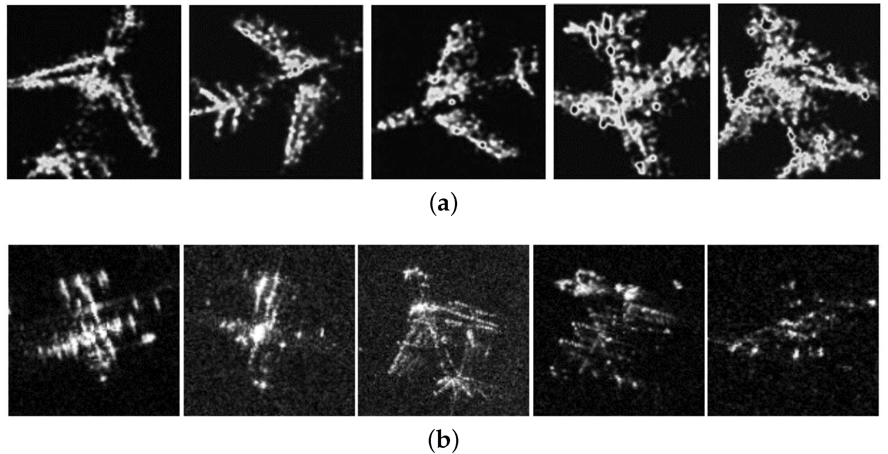
Figure 3.
Example of the ground truth of the validation data slice: (a) labelled location (the red cross) and angle (the green text), and (b) the ground truth of data slice in (a).
Figure 3.
Example of the ground truth of the validation data slice: (a) labelled location (the red cross) and angle (the green text), and (b) the ground truth of data slice in (a).
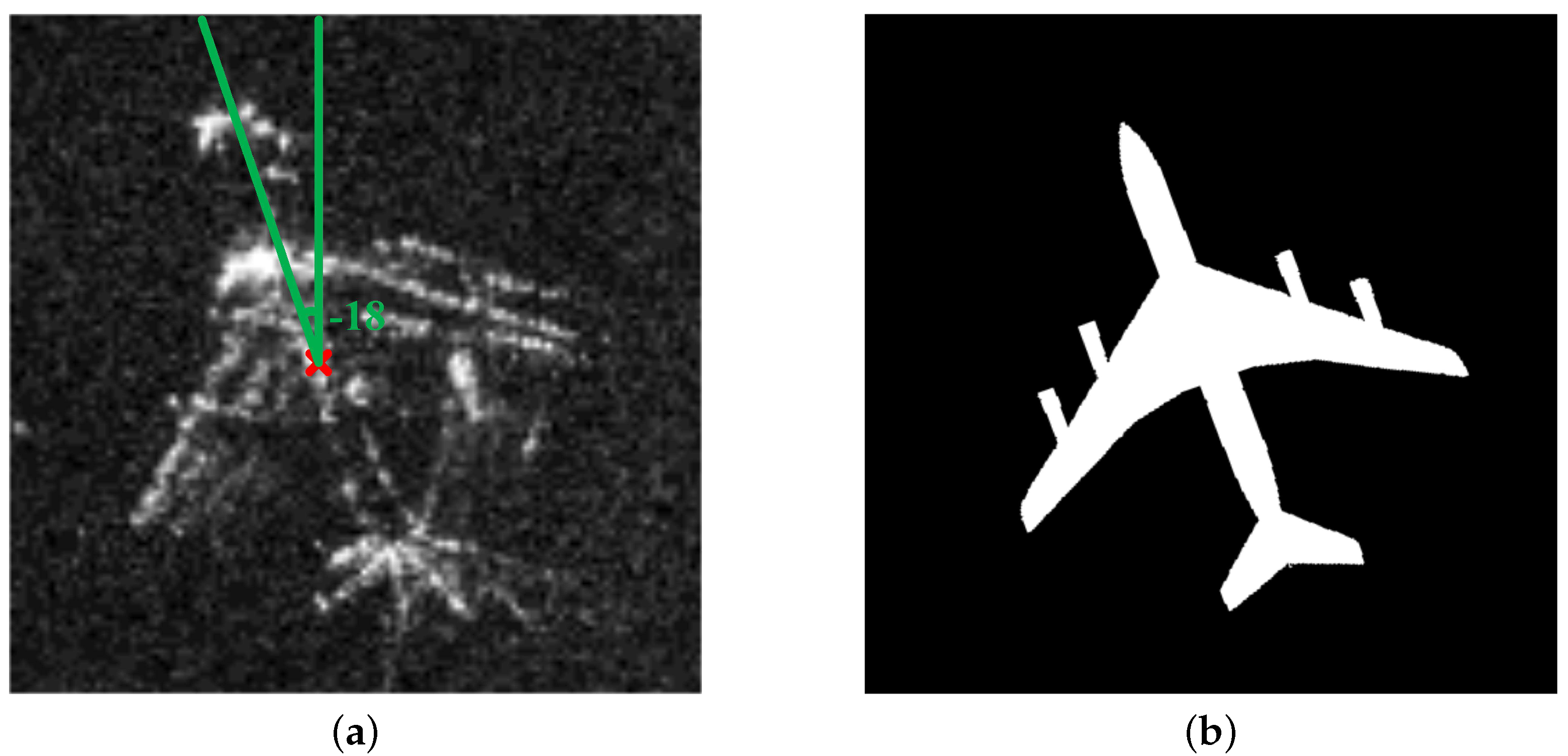
Figure 4.
Original shape templates of ten types of aircrafts in different poses.

Figure 5.
The top-view drawing of an aircraft and its binary shape: (a) Top-view drawing of an aircraft, and (b) Binary shape of the aircraft in (a).
Figure 5.
The top-view drawing of an aircraft and its binary shape: (a) Top-view drawing of an aircraft, and (b) Binary shape of the aircraft in (a).

Figure 6.
The workflow of the proposed aircraft reconstruction. , , and q represent the first hidden layer, the second hidden layer of DBM, and the shape of the object, respectively. DBM: deep Boltzmann machine; CFAR: constant false alarm rate; TILT: transform-invariant low-rank textures.
Figure 6.
The workflow of the proposed aircraft reconstruction. , , and q represent the first hidden layer, the second hidden layer of DBM, and the shape of the object, respectively. DBM: deep Boltzmann machine; CFAR: constant false alarm rate; TILT: transform-invariant low-rank textures.

Figure 7.
Examples of shape alignment. The first and second row represent the original templates and the results of shape alignment, respectively.
Figure 7.
Examples of shape alignment. The first and second row represent the original templates and the results of shape alignment, respectively.
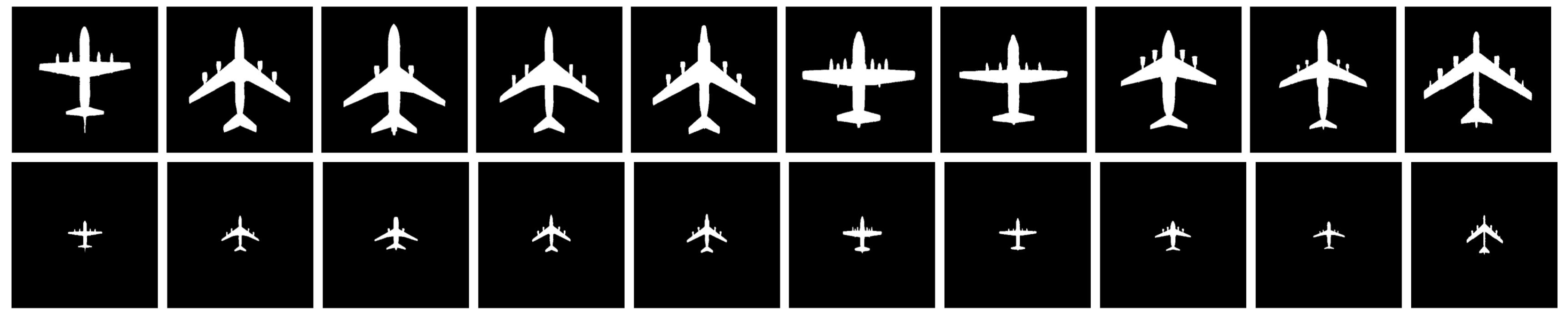
Figure 8.
The three-layered Deep Boltzmann Machine used for shape prior modelling.

Figure 9.
Approximate inference for visible and the first hidden layer in deep Boltzmann machine (DBM) training by Gibbs sampling.
Figure 9.
Approximate inference for visible and the first hidden layer in deep Boltzmann machine (DBM) training by Gibbs sampling.
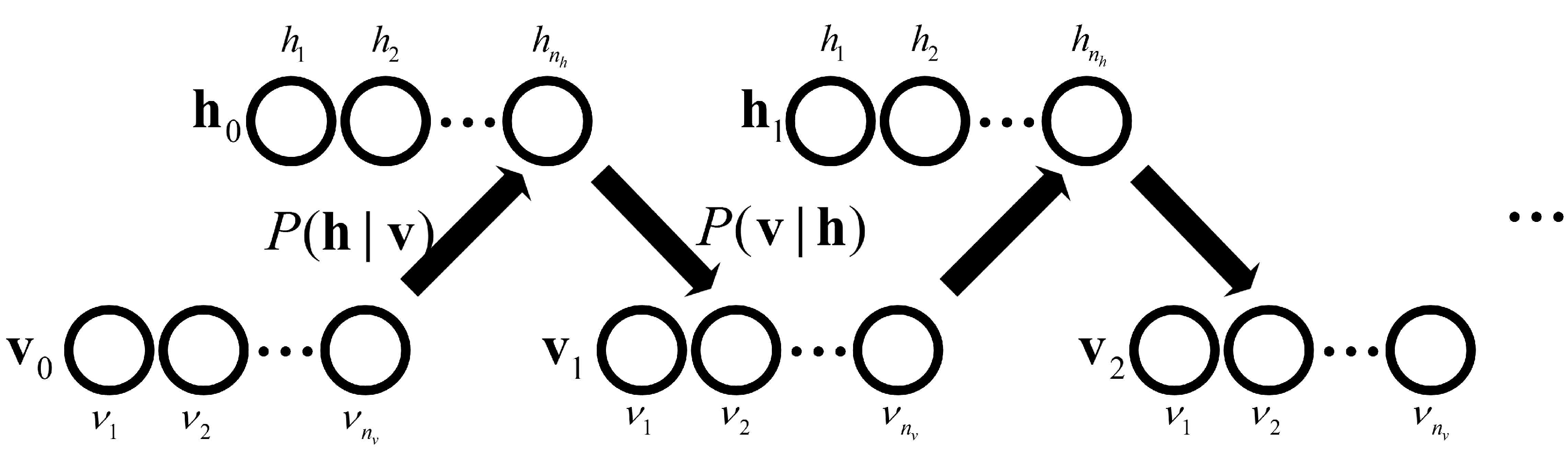
Figure 10.
Visualization of response intensity of units in the first hidden layer of the input image.
Figure 10.
Visualization of response intensity of units in the first hidden layer of the input image.
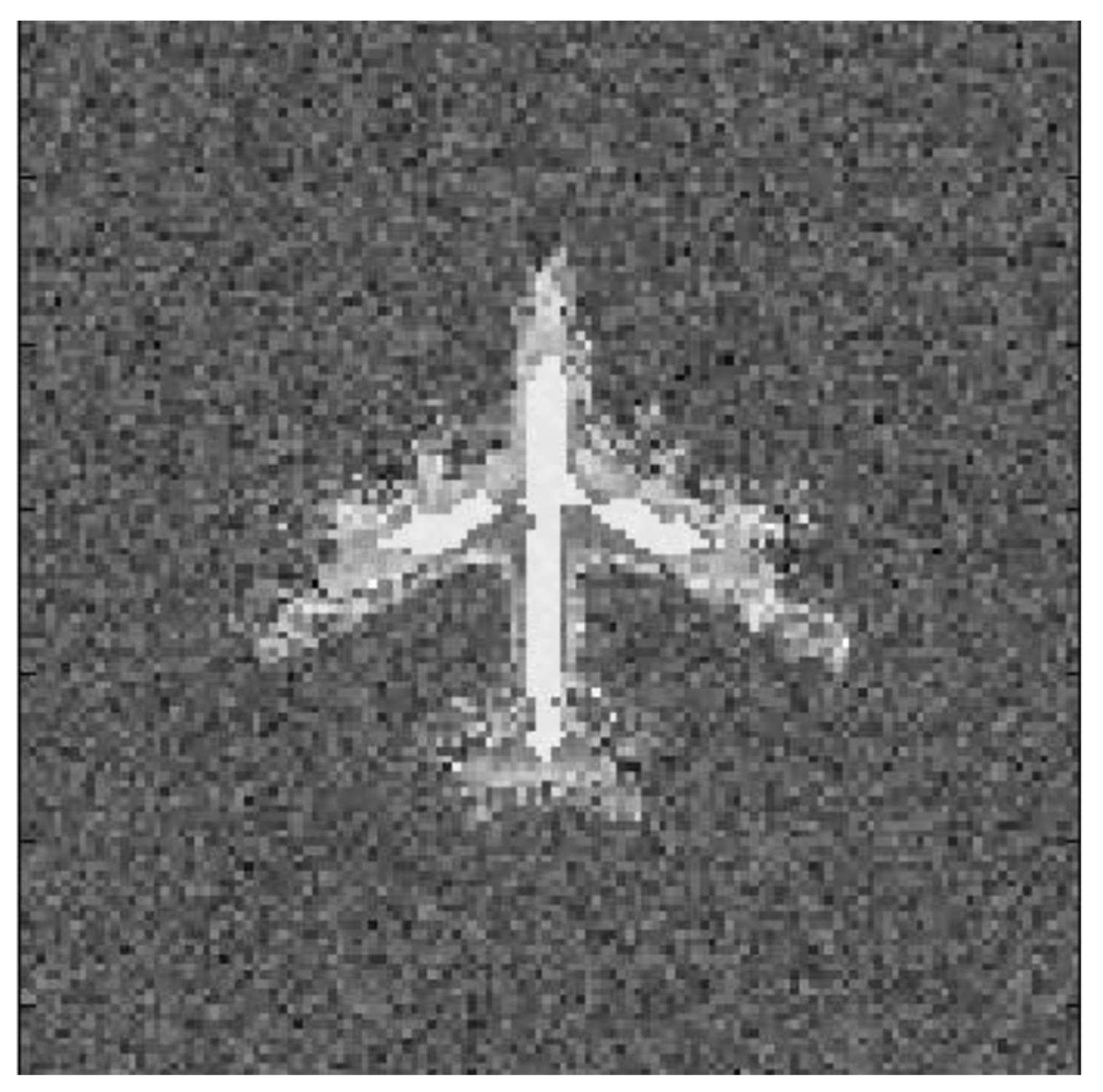
Figure 11.
Results of shape prior modelling for objects without and with absent parts. (a) Input image; (b) Deep shape prior.
Figure 11.
Results of shape prior modelling for objects without and with absent parts. (a) Input image; (b) Deep shape prior.
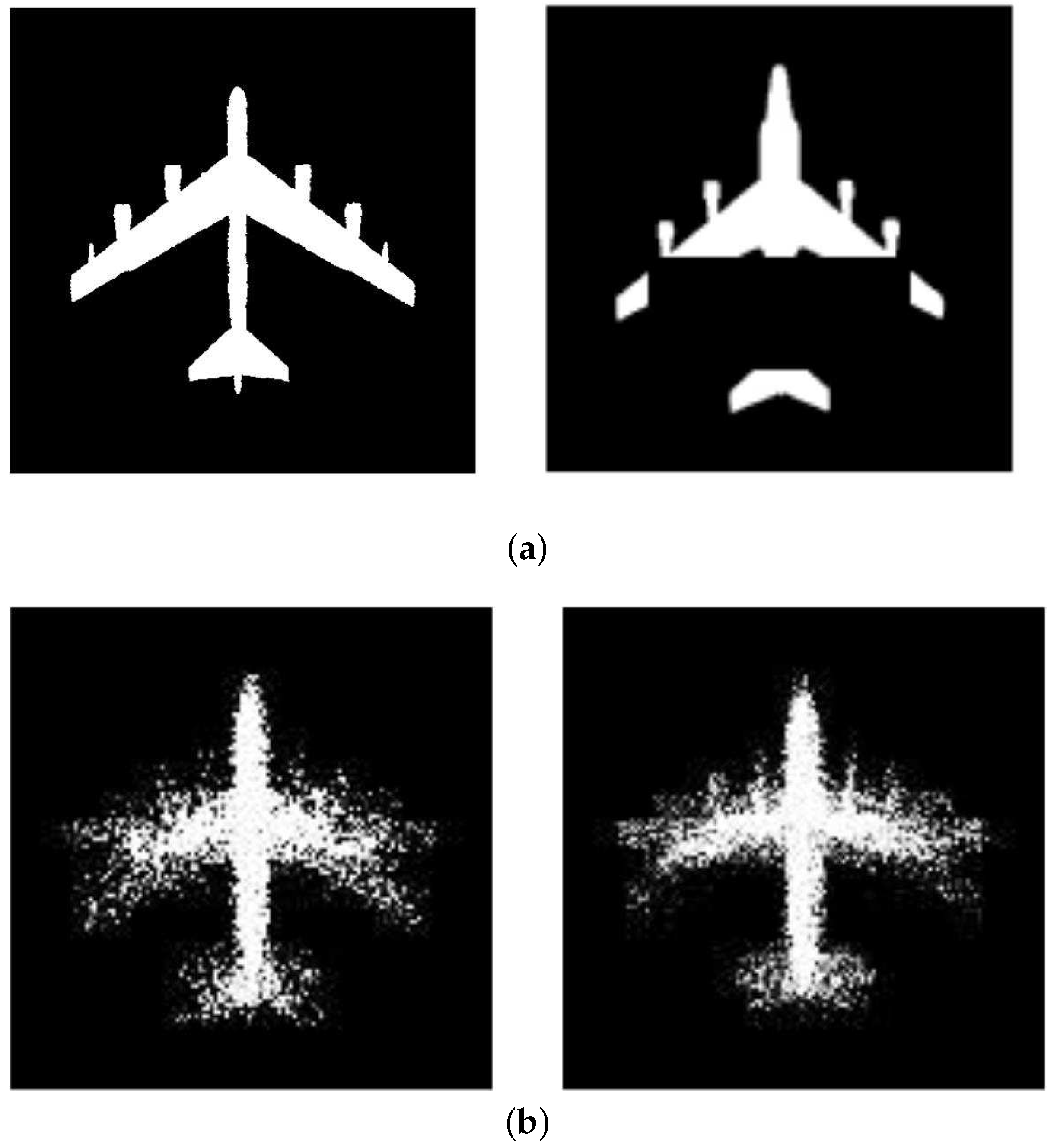
Figure 12.
Results of the pose estimation before reconstruction stage; (a) Original image slices. (b) Results after the pose estimation.
Figure 12.
Results of the pose estimation before reconstruction stage; (a) Original image slices. (b) Results after the pose estimation.
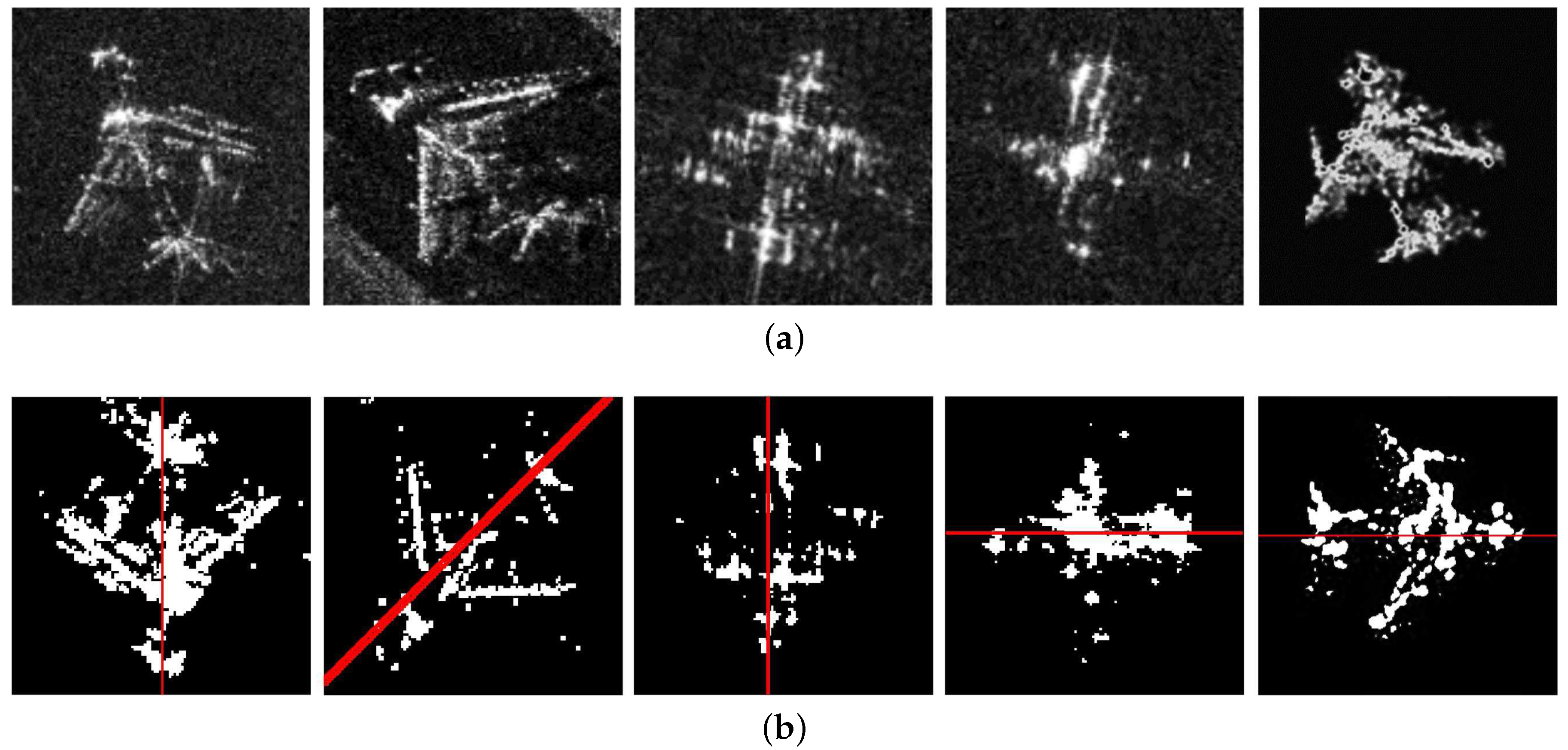
Figure 13.
Comparison of reconstruction results of different methods. (a,b) Reconstruction results of the graph cut method; (c,d) Reconstruction results of our method without the shape term. (e,f) Reconstruction results of Chan-Vese segmentation method. (g,h) Reconstruction results of our method.
Figure 13.
Comparison of reconstruction results of different methods. (a,b) Reconstruction results of the graph cut method; (c,d) Reconstruction results of our method without the shape term. (e,f) Reconstruction results of Chan-Vese segmentation method. (g,h) Reconstruction results of our method.

Figure 14.
Reconstruction results. Top row: Test data after turning the aircraft into the same pose. Middle row: Reconstruction results of SGACM. Bottom row: Reconstruction results of our method.
Figure 14.
Reconstruction results. Top row: Test data after turning the aircraft into the same pose. Middle row: Reconstruction results of SGACM. Bottom row: Reconstruction results of our method.


Table 1.
Examples of the image resolution. ST: Spotlight.
| Images | Mode | Resolution |
|---|---|---|
| Image I | ST-0.5 m | 0.230 m × 0.856 m |
| Image II | ST-1.0 m | 1.000 m × 1.123 m |
Table 2.
The accuracy of the coarse pose estimation with different preprocessing method. CFAR: constant false alarm rate.
Table 2.
The accuracy of the coarse pose estimation with different preprocessing method. CFAR: constant false alarm rate.
| Method | Accuracy (%) |
|---|---|
| No process | 72.0 |
| Histogram thresholding | 80.0 |
| CFAR | 95.0 |
Table 3.
Performance of different methods. PMP: percentage of misclassified pixels. SGACM: shape-based global minimization active contour model.
© 2017 by the authors. Licensee MDPI, Basel, Switzerland. This article is an open access article distributed under the terms and conditions of the Creative Commons Attribution (CC BY) license (http://creativecommons.org/licenses/by/4.0/).
Share and Cite
MDPI and ACS Style
Dou, F.; Diao, W.; Sun, X.; Zhang, Y.; Fu, K. Aircraft Reconstruction in High-Resolution SAR Images Using Deep Shape Prior. ISPRS Int. J. Geo-Inf. 2017, 6, 330. https://doi.org/10.3390/ijgi6110330
AMA Style
Dou F, Diao W, Sun X, Zhang Y, Fu K. Aircraft Reconstruction in High-Resolution SAR Images Using Deep Shape Prior. ISPRS International Journal of Geo-Information. 2017; 6(11):330. https://doi.org/10.3390/ijgi6110330
Chicago/Turabian StyleDou, Fangzheng, Wenhui Diao, Xian Sun, Yue Zhang, and Kun Fu. 2017. "Aircraft Reconstruction in High-Resolution SAR Images Using Deep Shape Prior" ISPRS International Journal of Geo-Information 6, no. 11: 330. https://doi.org/10.3390/ijgi6110330
Note that from the first issue of 2016, this journal uses article numbers instead of page numbers. See further details here.