A Post-Rectification Approach of Depth Images of Kinect v2 for 3D Reconstruction of Indoor Scenes


1
School of Electronic Engineering, Beijing University of Posts and Telecommunications, Beijing 100876, China
2
China State Construction Engineering Corporation Ltd. (CSCEC), Beijing 100876, China
*
Author to whom correspondence should be addressed.
ISPRS Int. J. Geo-Inf. 2017, 6(11), 349; https://doi.org/10.3390/ijgi6110349
Submission received: 22 August 2017
/
Revised: 17 October 2017
/
Accepted: 2 November 2017
/
Published: 13 November 2017
(This article belongs to the Special Issue 3D Indoor Modelling and Navigation)
Abstract
:3D reconstruction of indoor scenes is a hot research topic in computer vision. Reconstructing fast, low-cost, and accurate dense 3D maps of indoor scenes have applications in indoor robot positioning, navigation, and semantic mapping. In other studies, the Microsoft Kinect for Windows v2 (Kinect v2) is utilized to complete this task, however, the accuracy and precision of depth information and the accuracy of correspondence between the RGB and depth (RGB-D) images still remain to be improved. In this paper, we propose a post-rectification approach of the depth images to improve the accuracy and precision of depth information. Firstly, we calibrate the Kinect v2 with a planar checkerboard pattern. Secondly, we propose a post-rectification approach of the depth images according to the reflectivity-related depth error. Finally, we conduct tests to evaluate this post-rectification approach from the perspectives of accuracy and precision. In order to validate the effect of our post-rectification approach, we apply it to RGB-D simultaneous localization and mapping (SLAM) in an indoor environment. Experimental results show that once our post-rectification approach is employed, the RGB-D SLAM system can perform a more accurate and better visual effect 3D reconstruction of indoor scenes than other state-of-the-art methods.
1. Introduction
Indoor robot positioning, navigation, and semantic mapping depend on an accurate and robust 3D reconstruction of indoor scenes. A variety of techniques for 3D reconstruction of indoor and outdoor scenes have been developed, such as light detection and ranging (LiDAR) [1], stereo cameras [2], RGB and depth (RGB-D) cameras [3], and so on. Although a three-dimensional LiDAR could satisfy accuracy and robustness, such a system is very costly. Furthermore, the result is short of the important color information [1]. Stereo cameras can be utilized for 3D reconstruction of indoor scenes with low accuracy and a complex processing procedure [4]. Recently, the RGB-D camera has become a better alternative for 3D reconstruction of indoor scenes [5,6,7]. RGB-D cameras are novel sensing devices that capture RGB images along with corresponding depth images.
RGB-D cameras are sensing systems that capture RGB images along with per-pixel depth information. RGB-D cameras rely on either active stereo [8,9] or time-of-flight (ToF) sensing [10,11] to generate depth estimates at a large number of pixels. Kinect v2 (released in July 2014) has been more and more popular among the RGB-D cameras with properties of low-cost, accuracy, and robustness [3,12].
In addition to capturing high-quality color images, Kinect v2 employs a ToF technology to provide depth images. With the Kinect v2, many researchers have carried out related studies for 3D reconstruction in order to improve the accuracy, precision, and robustness [13,14,15,16]. In order to achieve that goal, the calibration of Kinect v2 plays an important role, but there are few off-the-shelf calibration methods for the Kinect v2 to take account of the reflectivity-related depth error, which is a key factor in influencing the accuracy and precision in 3D indoor scenarios [13,17,18]. Our contribution in this paper is to propose a post-rectification approach of the depth images according to the reflectivity-related depth error, which results in an improvement of the depth accuracy and precision shown in Section 5 and Section 6 in detail. Therefore, a better visual effect 3D reconstruction of indoor scenes is achieved than previous methods.
This paper is organized as follows: Section 2 discusses the related work on properties of Kinect v2 and using Kinect v2 for 3D reconstruction. Then we make a comprehensive analysis of the Kinect v2’s characteristics, including intrinsic parameters, extrinsic parameters, and lens distortions in Section 3. In Section 4, we propose the post-rectification approach of the depth images in detail. Furthermore, we carry out experiments and present the final results in Section 5. Finally, conclusions are offered in Section 6.
2. Related Work
Until now many studies on the Kinect v2 and its various applications have been carried out, such as a comparison between the two generations of Microsoft sensors—Kinect v1 and v2 [17,19,20], 3D reconstruction [3,7,13,21], and mobile robot navigation [14]. Within this section, the work related to the above is overviewed.
Sarbolandi et al. [19] present an in-depth comparison between the two versions of the Kinect range sensor. While the Kinect v1 employs the structured-light method on its depth sensor, the Kinect v2 uses time-of-flight technology to obtain the depth information. They make a comprehensive and detailed analysis of error sources with two Kinect sensors, including the intensity-related distance error, i.e., reflectivity-related depth error, only for the Kinect v2. By contrasting experiments, the Kinect v2 shows a lower systematic distance error and greater insensitivity to the ambient background light.
Through a large number of accuracy and precision experiments, Gonzalez-Jorge et al. [22] obtain a conclusion that within a 2 m range, the Kinect v2 keeps all result values below 8 mm in precision, with values always lower than 5 mm in accuracy. However, the precision should be further improved for 3D indoor scenario re-construction. Moreover, the accuracy should also be improved for creating a better point cloud map.
Lindner et al. [23,24] make an in-depth study on the reflectivity-related depth error for a ToF camera. A planar checkerboard pattern with different levels of reflectivity is used to calibrate a single ToF camera.
The Kinect v2 uses time-of-flight technology for measuring distances [20]. From the physical and mathematical point of view, Valgma et al. [20] analyze the depth-measuring principle in detail. The pinhole camera model, camera lens’ radial distortion, and alignment of the depth and color sensors are individually discussed. Afterward, they state six important factors that can cause errors in depth measurements in real operation.
Rodríguez-Gonzálvez et al. [25] first developed a radiometric calibration equation for the depth sensor for the Kinect v2 based on reflectance to convert the recorded digital levels into physical values. The results confirm that the quality of the method is valid for exploiting the radiometric possibilities of this low-cost depth sensor to agricultural and forest resource evaluation. However, they have not investigated the specific accuracy and precision with the Kinect v2 in the application of indoor environments.
Therefore, in this paper, we propose a new post-rectification approach that is inspired by [17,19,25]. The main contribution of our proposed algorithm is based on the reflectivity-related depth error with Kinect v2, which is newly-applied in improving 3D reconstruction accuracy in indoor environments.
3. Kinect v2 Sensor Presentation
3.1. Characteristics of the Kinect v2
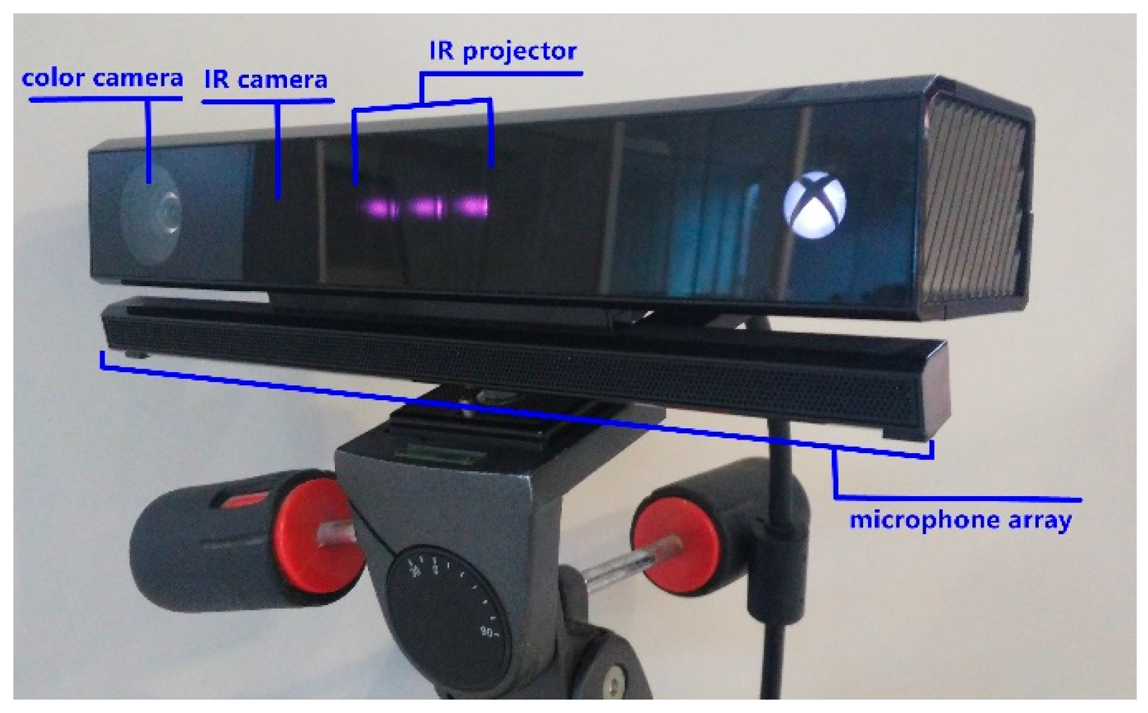
As an RGB-D sensor, the Kinect v2 is the second-generation Kinect by Microsoft, released in July 2014. Equipped with a color camera, depth sensor (including infrared (IR) camera and IR projector) and a microphone array, the Kinect v2 can be used to sense color images, depth images, IR images and audio information. The hardware structure is shown in Figure 1. The detailed technical specifications are summarized in Table 1 [17,22,25].
3.2. Pinhole Camera Model
A color camera and IR camera are respectively regarded with the pinhole camera model. In this model, there are four coordinate systems—the world coordinate system, camera coordinate system, image physics coordinate system, and image pixel coordinate system. The pinhole camera model implies that points in a 3D world are mapped onto the image plane of the camera [21]. To put it another way, it is to transport a point in the 3D world coordinate system to the 2D image pixel coordinate system (Figure 2).
Let P(X,Y,Z) be a 3D point in the world coordinate system. While Pc(Xc,Yc,Zc) is its corresponding point in the camera coordinate system, P′(X′,Y′) is the corresponding image physics coordinate, and the corresponding image pixel coordinate is p(u,v).
According to the pinhole camera model [21], we can obtain the following formula:
Equation (1) describes the projection relation from world coordinate P(X,Y,Z) to image pixel coordinate p(u,v). K is the camera intrinsic matrix, and fx, fy, u0, and v0 are intrinsic camera parameters. R and t are camera extrinsic parameters.
3.3. Distortion Model of Camera Lens
There are two different kinds of distortions of the camera lens in the process of camera imaging [21]. One is a radial distortion caused by shape distortion of a lens. The other is where the lens is not completely parallel to the imaging plane, forming tangential distortion.
Regarding the above two distortions, we use the following formulas to correct distortion, respectively:
In Equation (2), (x,y) is the uncorrected point coordinate, r2 is equal to x2 + y2. (xrad,yrad) is the coordinate after correcting radial distortion, (xtan,ytan) is the coordinate after correcting tangential distortion, and (xcorrected,ycorrected) is the coordinate after correcting above two kinds of distortions. The k1, k2, k3, p1, and p2 are the distortion coefficients which are referred to in Table 2.
3.4. Depth Sensor
There are several error sources influencing the depth sensor of the Kinect v2. Table 3 shows the error sources for depth sensor of the Kinect v1 and Kinect v2 [7,19,20].
Among the error sources, except the intensity-related distance error, also called reflectivity-related error and flying pixel, the others influence not only the Kinect v1, but also the Kinect v2, on depth sensing. In the next section, a post-rectification approach of the depth images is raised, aiming at reducing the reflectivity-related effect for the Kinect v2 on the depth measurement.
4. Method
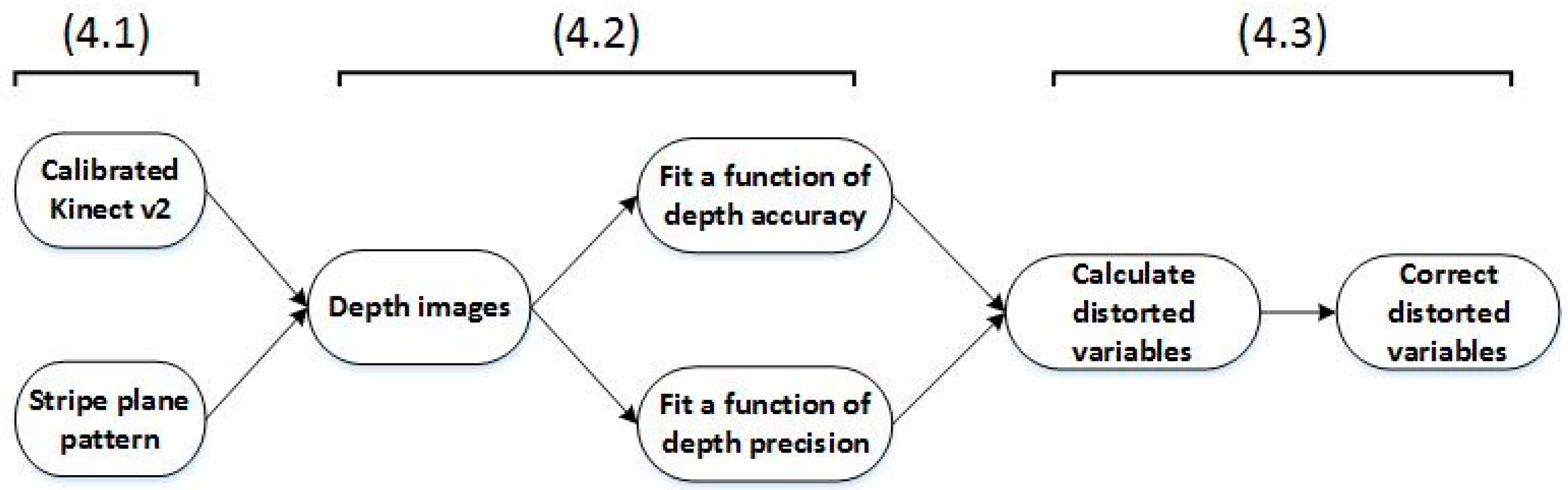
In this section, we propose the post rectification approach in detail. An overview is illustrated in Figure 3.
4.1. Calibrate the Kinect v2 and Prepare the Stripe Plane Pattern
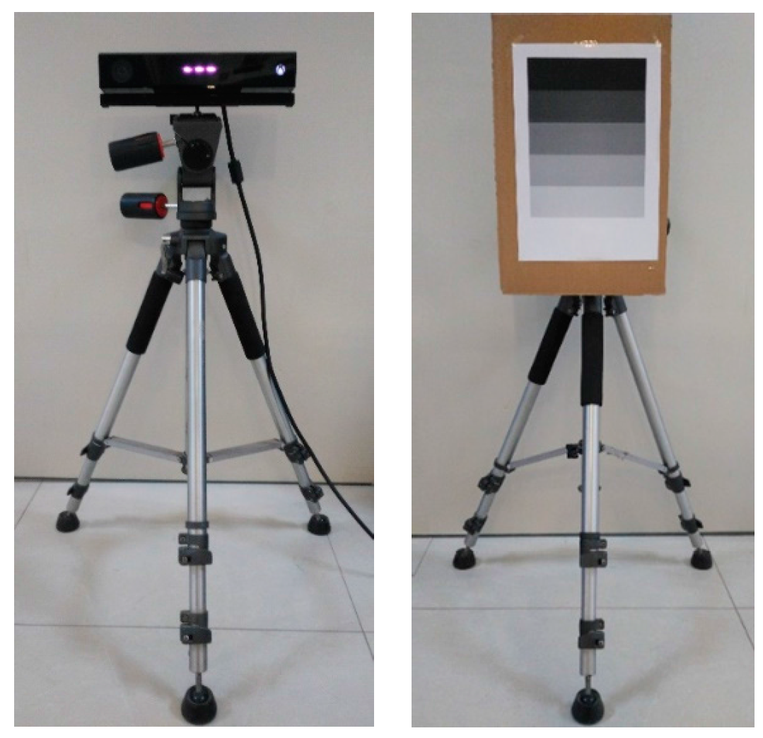
In this paper, we equipped our computer with the Ubuntu 14.04 operating system and libfreenect2 [26], which is the driver for the Kinect v2. Then we printed a chessboard calibration pattern (5 × 7 × 0.03) [18] on A4 paper. Additionally, we used two tripods, one for holding the calibration pattern, and another one for holding the Kinect v2 sensor to calibrate the color, infrared, sync, and depth successively at two distances: 0.9 m and 1.8 m. It is noted that the pinhole camera model is used to explain the corresponding parameters of calibrating the Kinect v2 under different reflectivity.
Actually, there is a possible geo-referencing problem in our post-rectification method. However, in a short distance, the camera can be conducted perfectly orthogonally. Even in the worst condition there is an incidence angle of approximately 8° in its frame edges, which is equivalent to an error of 0.13% for the reflectance value. Therefore, the performance of our proposed algorithm is not affected.
We firstly designed and utilized a stripe plane pattern with different grayscales to investigate the relationship of reflectivity and measured depth. The squared panel divided the gray values into six levels of 100% black, 80% black, 60% black, 40% black, 20% black, and 0% black (white). In the stripe plane pattern, the top strip is printed with 0.0013, decreasing in five steps to 0.9911 (white) from top to bottom with the same size (Figure 4a). This approach is inspired by the Ringelmann card that is usually used in the reflectance calibration. It is noted that the panel is calibrated for wavelengths of 827 nm to 849 nm. These wavelengths are the expected range for the Kinect 2. As we know, the reflectivity is related to the wavelength, so we chose a mean value as the estimated reflectance factor when the wavelength is 838 nm, which is shown in Table 3.
4.2. Capture Depth Images and Fit Functions of Depth Accuracy and Precision, Respectively
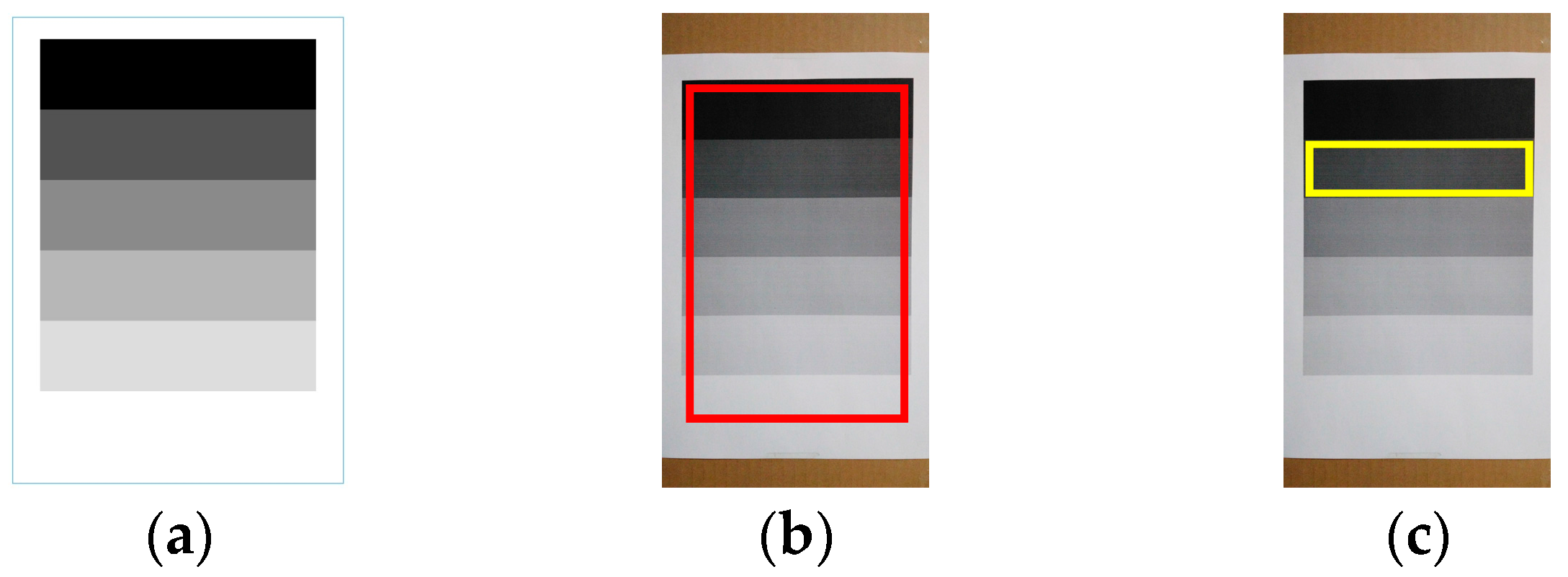
At the same reflectivity, we took the grayscale of 80% black at different distances in the operative measuring range as an example. The region to be studied is presented in Figure 4c with a yellow box.
We fixed the calibrated Kinect v2 sensor to a stable tripod, and mounted the stripe plane pattern to the other tripod. As shown in Figure 5, the front panel of the Kinect v2 sensor and the stripe plane pattern are always maintained in parallel, both perpendicular to the ground, using a large triangular rule to guarantee alignment. The stripe plane pattern is progressively moved away from the Kinect v2 sensor in the operative measuring range with a step length of x meters (less than 0.20 m). Therefore, L sets of depth images of the yellow box region are captured. One set contains N (no less than 1) depth images.
Step 1: we calculate a mean depth image and an offset matrix of each set of depth images:
where L is the quantity of the depth image sets of the yellow box region captured, i is the sequence number of sets, and N is the quantity of depth images that each set contains, j the sequence number of depth images of each set. Mij is every depth image of each set, and Mi is the calculated mean depth image of each set. The ground truth matrix is expressed as Mgi (measured by the flexible ruler). Then we obtain an offset matrix Moi for each distance.
Step 2: we average pixel values of each offset matrix Moi:
where R is the number of rows of each yellow box region of each offset matrix Moi that varies with different distances, p the sequence number of the rows, and C is the number of columns of each yellow box region of each offset matrix Moi, q the sequence number of the columns. In the offset matrix Moi, each pixel value offset to the ground truth in the yellow box is represented as mpq. mi is the expectation of each offset matrix Moi.
Step 3: based on Equations (4) and (5), we compute the standard deviation si of the offset matrix Moi for each distance:
Step 4: we utilize a fitting function three-term sum of sine (Equation (7)) to model the expectation of the offset matrix Moi (Figure 8a) and a linear polynomial (Equation (8)) to model the standard deviation of the offset matrix Moi (Figure 8b), which is dependent on the above analysis:
where d is the distance, md is the offset expectation corresponding to the distance, sd is the offset standard deviation corresponding to the distance. a1, a2, a3, b1, b2, b3, c1, c2, and c3 are coefficients to be determined in Equation (7). t1 and t2 are coefficients to be determined in Equation (8).
4.3. Correct Depth Images
For different distances, we correct the depth image based on Equation (7). The corrected yellow box region depth image is:
where Md is the depth image corresponding to the distance. Then, based on Equations (4)–(6), we can calculate mcorr and scorr. mcorr represents the corrected expectation of the offset matrix and scorr represents the standard deviation. The depth accuracy of the Kinect v2 is evaluated by the expectation of an offset matrix of the depth image, and the depth precision is evaluated by the standard deviation [20,22]. In the next section, we apply the post-rectification approach to RGB-D SLAM [6] in an indoor environment to prove its real effect.
5. Experiments and Results
We conducted experiments in an office room with essentially constant ambient background light. It is noted that we spent 40 min to pre-heat the Kinect v2 sensor, for the sake of eliminating the temperature drift effect [13,20].
Since both the accuracy and the precision will decrease with the increasing measuring range [17], and indoor environments are usually small, like our office room environment, the operative measuring range in this paper is no more than 2 m. The tripod with stripe plane pattern is progressively moved away from the Kinect v2 sensor, from 0.45 m to 2.10 m, with a 0.15 m step width. Therefore, 10 sets of depth images of the yellow box region are captured. One set contains five depth images.
We obtain three depth images successively at the first three distance: 0.45 m, 0.60 m, and 0.75 m. By analyzing the same region of the stripe plane pattern (red box in Figure 4b) at these three distances, three visualized depth images of the red box region are illustrated in the Figure 6a–c. It is noted that the color-bar indicates the pixel values of the depth image. We reveal that at a short distance, an invalid null value (pixel value 0) is easy to obtain in high-reflectivity regions at the bottom of the red box, as shown in Figure 6a,b. Summarized, the minimum operative measuring distance is located between 0.60 m and 0.75 m in our indoor environment, which is larger than the official given value of 0.5 m.
In order to avoid the effect of invalid null value and carry out reliable studies, the distance is adjusted from 0.75 m to 2.10 m, with the same 0.15 m step width in the following experiments.
5.1. Same Distance, but Different Reflectivity
At the same distance, six kinds of different reflectivity in the red box on the stripe plane pattern (Figure 4b) affect the measured distance obviously. As shown in the top of Figure 7, with the reflectivity increases (row axis from small to large in Figure 7, or rows of the red box, top to bottom in Figure 4b), the measured distance becomes smaller at a distance of 0.75 m. Figure 6c also illustrates the fact for a distance of 0.75 m in the front view. Furthermore, it is presented clearly in the side view at a distance of 0.75 m in the bottom of Figure 7.
5.2. Same Reflectivity, but Different Distances
Based on Section 4, we carry out experiments with the post-rectification approach to investigate the relationship between the measured depth and six kinds of reflectivity on the stripe plane pattern (Figure 8), respectively. The experimental results are shown in Table 4, where mcorr is the standard deviation of the depth information difference between the corrected and the ground-truth, Scorr is the expectation of mcorr, m is the standard deviation of the depth information difference between the un-corrected values and the ground-truth, and s is the expectation of m. It should be noted that m is achieved by using the post-rectification that was proposed by [23].
It is noted that in a short distance, the camera can be conducted perfectly orthogonal. Even in the worst condition, an incidence angle approximately 8° in its frame edges, which is equivalent to an error of 0.13% for the reflectance value. Therefore, the performance of our proposed algorithm is not affected.
As bold data show in Table 4, for the depth accuracy, we obtain the best experimental results below 1 mm at a grayscale of 40% from a distance 0.75 m to 2.10 m. Correspondingly, at a high reflectivity at a grayscale of 0%, the depth accuracy is below 3 mm, which is the whole depth accuracy. It is noted that our accuracy is better than the result (its accuracy is 5 mm) which is indicated in [22]. Moreover, the experimental results in [22] were achieved by a classic rectification measurement. Furthermore, for the depth precision, we obtain the best experimental results below 3 mm at a grayscale of 60% from a distance 0.75 m to 2.10 m. At a low reflectivity at a grayscale of 100%, the depth precision is below 6 mm, which is the whole depth precision.
Furthermore, after analyzing Figure 7b and Table 4, we can indicate that our proposed post-rectification algorithm is a linear model, as we stated in the previous section. This is because Scorr is the same with s.
There are two possible explanations for intensity-related effect for Kinect v2. One assumption is a specific variant of a multi-path effect, and the other one puts this effect down to the nonlinear pixel response for low amounts of incident intensity.
Finally, following the instructions proposed in Section 4.2, we complete the calibration of the Kinect v2 and acquire a series of parameters that the Kinect v2 needs in Table 5.
5.3. Application for RGB-D SLAM System
In the sake of proving the effect of the post-rectification approach, we apply it to RGB-D SLAM [6] in an indoor environment. Our indoor scene under experiment is around 1.4 m away from the Kinect sensor, so we calculate the expectation of offset of six kinds of reflectivity according to Section 4 at a distance 1.4 m. The results are shown in Table 6.
As shown in Table 6, with the decrease of reflectivity (an increase of the grayscale level), the expectation of offset is progressively rising. Then we average those six values of expectation to be the deviation of this indoor scene. After correction, an average of 118 mm deviation is eliminated. Via the offline RGB-D SLAM method, Figure 9 presents two kinds of point clouds magnified by the same multiples before and after correction by using our proposed method. Therefore, it is obvious that, after correction, the scene is closer to the Kinect v2 sensor than before in the point cloud, which indicates that the depth accuracy of the point cloud is improved. Moreover, an excellent visual effect point cloud of this indoor scene is displayed in Figure 10. The line in the middle of the top overall view is the trajectory of Kinect v2. The bottom is a side view at the red point position of the trajectory in the top overall view.
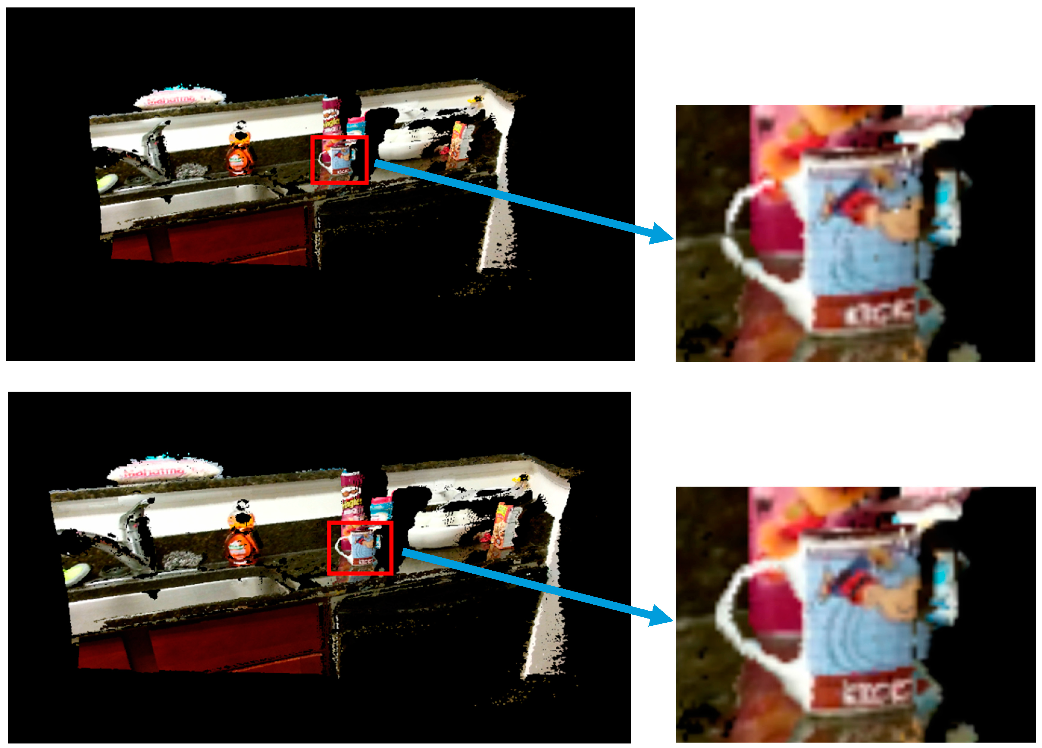
Furthermore, we apply the post rectification approach to the George Mason University (GMU) Kitchen Dataset [27], which is captured by a Kinect v2. Figure 11 shows the point cloud before and after correction by using our proposed method. According to the two red rectangles of Figure 11, we can find that the bottle is larger after using our post-rectification, while losing little information, which can support more useful scene information than without post-rectification. This is due to using precision depth data.
6. Conclusions
Within this work, we analyze the relationship between the measured distance of the depth image and reflectivity of the indoor scene for the Kinect v2 depth sensor in detail. Based on the analysis of reflectivity-related depth error, this paper proposes a post-rectification methodology to correct the depth images. We utilize a calibrated Kinect v2 and a stripe plane pattern to capture depth images of the indoor environment. Then, the functions of depth accuracy and precision are fitted respectively with the depth images. Finally, according to the fitting functions, we can correct the dataset’s depth images to obtain more accurate and precise depth images so as to generate a point cloud. As the experimental results show, the accuracy is below 3 mm from a distance of 0.75 m to 2.10 m, which is 2 mm lower than that in [22]. Moreover, the precision is below 6 mm, which is 2 mm lower than that in [22]. Therefore, our proposed post-rectification approach outperforms the previous work, which will be useful for high-precision 3D mapping of the indoor environments, as well as subsequent semantic segmentation and semantic understanding.
Further studies will consider applying the post rectification approach to 3D reconstruction of indoor scenes in real-time with the Kinect v2 sensor.
Acknowledgments
The project sponsored by the National Key Research and Development Program (no. 2016YFB0502002), the National Natural Science Foundation of China (no. 61401040), and the Beijing University of Posts and Telecommunications Young Special Scientific Research Innovation Plan (2016RCGD11).
Author Contributions
Jichao Jiao and Zhongliang Deng conceived and designed the experiments; Libin Yuan performed the experiments; Weihua Tang analyzed the data; Qi Wu contributed analysis tools; Jichao Jiao wrote the paper.
Conflicts of Interest
The authors declare no conflict of interest.
References
- Wu, B.; Yu, B.; Wu, Q.; Yao, S.; Zhao, F.; Mao, W. A graph-based approach for 3D building model reconstruction from airborne LiDAR point clouds. Remote Sens. 2017, 9, 92. [Google Scholar] [CrossRef]
- Kuhnert, K.-D.; Stommel, M. Fusion of stereo-camera and pmd-camera data for real-time suited precise 3d environment reconstruction. In Proceedings of the 2006 IEEE/RSJ International Conference on Intelligent Robots and Systems, Beijing, China, 9–15 October 2006; pp. 4780–4785. [Google Scholar]
- Lachat, E.; Macher, H.; Mittet, M.; Landes, T.; Grussenmeyer, P. First experiences with Kinect v2 sensor for close range 3D modelling. Int. Arch. Photogramm. Remote Sens. Spat. Inf. Sci. 2015, 40. [Google Scholar] [CrossRef]
- Lee, D. Optimizing Point Cloud Production from Stereo Photos by Tuning the Block Matcher. Available online: https://erget.wordpress.com/2014/05/02/producing-3d-point-clouds-from-stereo-photos-tuning-the-block-matcher-for-best-results/ (accessed on 20 August 2017).
- Henry, P.; Krainin, M.; Herbst, E.; Ren, X.; Fox, D. RGB-D mapping: Using Kinect-style depth cameras for dense 3D modeling of indoor environments. Int. J. Robot. Res. 2012, 31, 647–663. [Google Scholar] [CrossRef]
- Endres, F.; Hess, J.; Sturm, J.; Cremers, D.; Burgard, W. 3-D mapping with an RGB-D camera. IEEE Trans. Robot. 2014, 30, 177–187. [Google Scholar] [CrossRef]
- Valgma, L. 3d Reconstruction Using Kinect v2 Camera. Bachelor’s Thesis, University of Tartu, Tartu, Estonia, 2016. [Google Scholar]
- Konolige, K. Projected texture stereo. In Proceedings of the 2010 IEEE International Conference on Robotics and Automation (ICRA), Anchorage, AK, USA, 3–8 May 2010; pp. 148–155. [Google Scholar]
- PrimeSense. Light Coding Technology. Available online: https://en.wikipedia.org/wiki/PrimeSense (accessed on 20 March 2016).
- Canesta. Time-of-Flight Technology. Available online: https://en.wikipedia.org/wiki/Canesta (accessed on 17 January 2017).
- MESA Imaging. ToF (Time-of-Flight). Available online: https://en.wikipedia.org/wiki/MESA_Imaging (accessed on 20 August 2017).
- Butkiewicz, T. Low-cost coastal mapping using Kinect v2 time-of-flight cameras. Oceans-St. John’s 2014, 2014, 1–9. [Google Scholar]
- Lachat, E.; Macher, H.; Landes, T.; Grussenmeyer, P. Assessment and calibration of a RGB-D camera (kinect v2 sensor) towards a potential use for close-range 3D modeling. Remote Sens. 2015, 7, 13070–13097. [Google Scholar] [CrossRef]
- Fankhauser, P.; Bloesch, M.; Rodriguez, D.; Kaestner, R.; Hutter, M.; Siegwart, R. Kinect v2 for mobile robot navigation: Evaluation and modeling. In Proceedings of the 2015 International Conference on Advanced Robotics (ICAR), Istanbul, Turkey, 27–31 July 2015; pp. 388–394. [Google Scholar]
- Choi, S.; Zhou, Q.-Y.; Koltun, V. Robust reconstruction of indoor scenes. In Proceedings of the IEEE Conference on Computer Vision and Pattern Recognition, Boston, MA, USA, 7–12 June 2015; pp. 5556–5565. [Google Scholar]
- Wasenmüller, O.; Meyer, M.; Stricker, D. Augmented reality 3d discrepancy check in industrial applications. In Proceedings of the 2016 IEEE International Symposium on Mixed and Augmented Reality (ISMAR), Merida, Mexico, 19–23 September 2016; pp. 125–134. [Google Scholar]
- Pagliari, D.; Pinto, L. Calibration of kinect for xbox one and comparison between the two generations of Microsoft sensors. Sensors 2015, 15, 27569–27589. [Google Scholar] [CrossRef] [PubMed] [Green Version]
- Wiedemeyer, T. Tools for Using the Kinect One (Kinect v2) in ROS. Available online: https://github.com/code-iai/iai_kinect2 (accessed on 20 August 2017).
- Sarbolandi, H.; Lefloch, D.; Kolb, A. Kinect range sensing: Structured-light versus time-of-flight kinect. Comput. Vis. Image Underst. 2015, 139, 1–20. [Google Scholar] [CrossRef]
- Wasenmüller, O.; Stricker, D. Comparison of Kinect v1 and v2 Depth Images in Terms of Accuracy and Precision. In Proceedings of the Asian Conference on Computer Vision Workshop (ACCV workshop), Taipei, Taiwan, 20–24 November 2016; Springer: Cham, Switzerland, 2016. [Google Scholar]
- Lawin, F.J. Depth Data Processing and 3D Reconstruction Using the Kinect v2. Master’s Thesis, Linköping University, Linköping, Sweden, 2015. [Google Scholar]
- Gonzalez-Jorge, H.; Rodríguez-Gonzálvez, P.; Martínez-Sánchez, J.; González-Aguilera, D.; Arias, P.; Gesto, M. Metrological comparison between Kinect I and Kinect II sensors. Measurement 2015, 70, 21–26. [Google Scholar] [CrossRef]
- Lindner, M.; Kolb, A. Calibration of the intensity-related distance error of the PMD ToF-camera. Opt. East 2007, 2007, 67640W:1–67640W:8. [Google Scholar]
- Lindner, M.; Schiller, I.; Kolb, A.; Koch, R. Time-of-flight sensor calibration for accurate range sensing. Comput. Vis. Image Underst. 2010, 114, 1318–1328. [Google Scholar] [CrossRef]
- Rodríguez-Gonzálvez, P.; González-Aguilera, D.; González-Jorge, H.; Hernández-López, D. Low-Cost Reflectance-Based Method for the Radiometric Calibration of Kinect 2. IEEE Sens. J. 2016, 16, 1975–1985. [Google Scholar] [CrossRef]
- Blake, J.; Echtler, F.; Kerl, C. Open Source Drivers for the Kinect for Windows v2 Device. Available online: https://github.com/OpenKinect/libfreenect2 (accessed on 20 August 2017).
- Georgakis, G. Multiview RGB-D Dataset for Object Instance Detection. Available online: http://cs.gmu.edu/~robot/gmu-kitchens.html (accessed on 20 August 2017).
Figure 1.
Kinect v2 sensor working on a photographic tripod.

Figure 2.
Pinhole camera model.
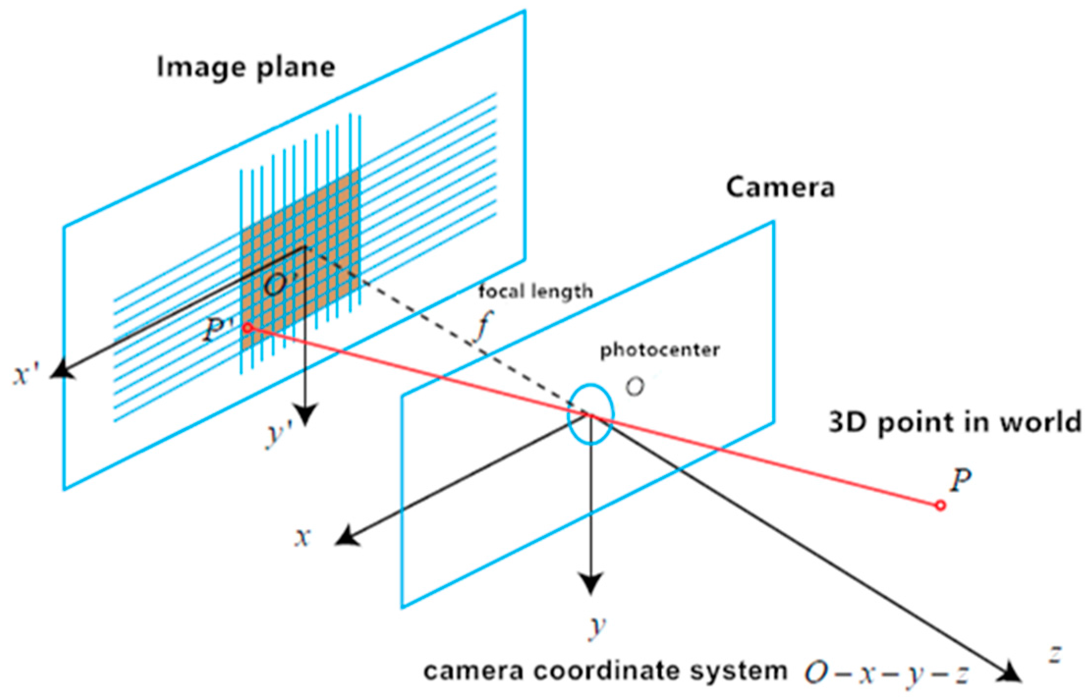
Figure 3.
The post-rectification approach overview.

Figure 4.
Stripe plane pattern with different grayscales printed on A4 paper: (a) stripe plane pattern on A4 paper; (b) red box region; and (c) yellow box region.
Figure 4.
Stripe plane pattern with different grayscales printed on A4 paper: (a) stripe plane pattern on A4 paper; (b) red box region; and (c) yellow box region.

Figure 5.
Setup of the method: Kinect v2 (left); stripe plane pattern (right).

Figure 6.
Visualized depth images of the red box region at different distances (front view): (a) 0.45 m; (b) 0.60 m; and (c) 0.75 m.
Figure 6.
Visualized depth images of the red box region at different distances (front view): (a) 0.45 m; (b) 0.60 m; and (c) 0.75 m.
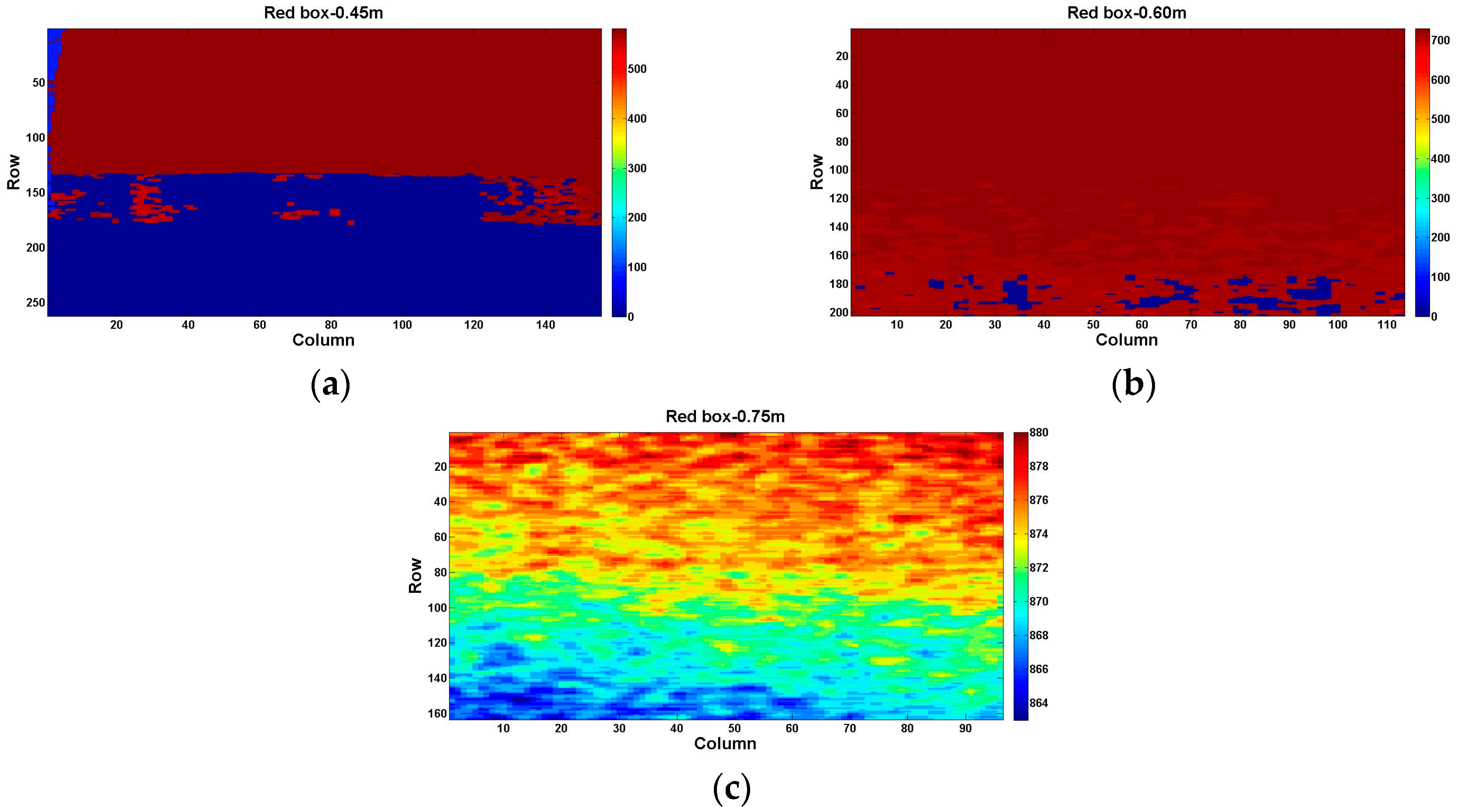
Figure 7.
Red box region at distance 0.75 m: 3D view (top); side view (bottom).

Figure 8.
Expectation (a) and standard deviation (b) of offset matrix Moi under the same reflectivity and different distances.
Figure 8.
Expectation (a) and standard deviation (b) of offset matrix Moi under the same reflectivity and different distances.
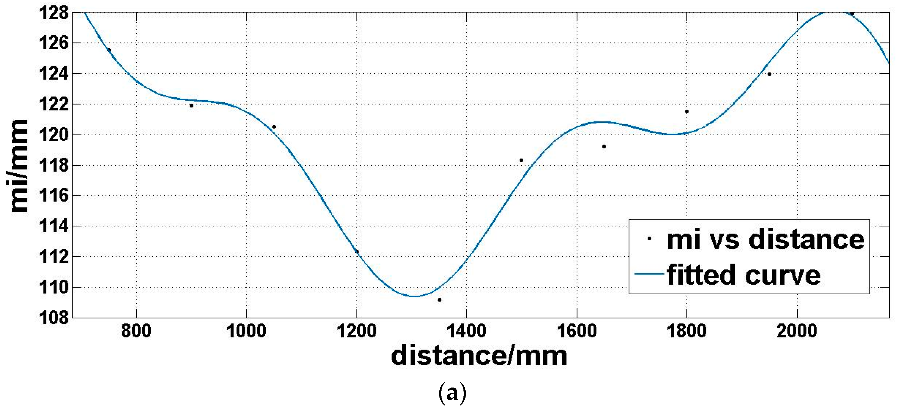
Figure 9.
Point cloud of an indoor scene before (top) and after (bottom) correction using the post-rectification approach.
Figure 9.
Point cloud of an indoor scene before (top) and after (bottom) correction using the post-rectification approach.
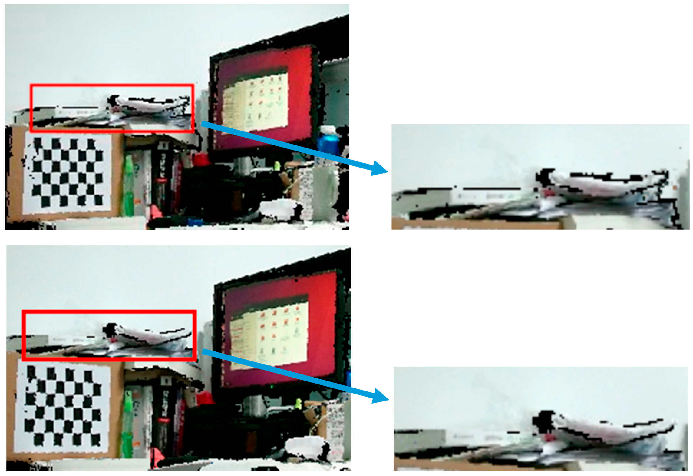
Figure 10.
Point cloud of this indoor scene: overall view (top); a side view at the red point position in the overall view (bottom).
Figure 10.
Point cloud of this indoor scene: overall view (top); a side view at the red point position in the overall view (bottom).
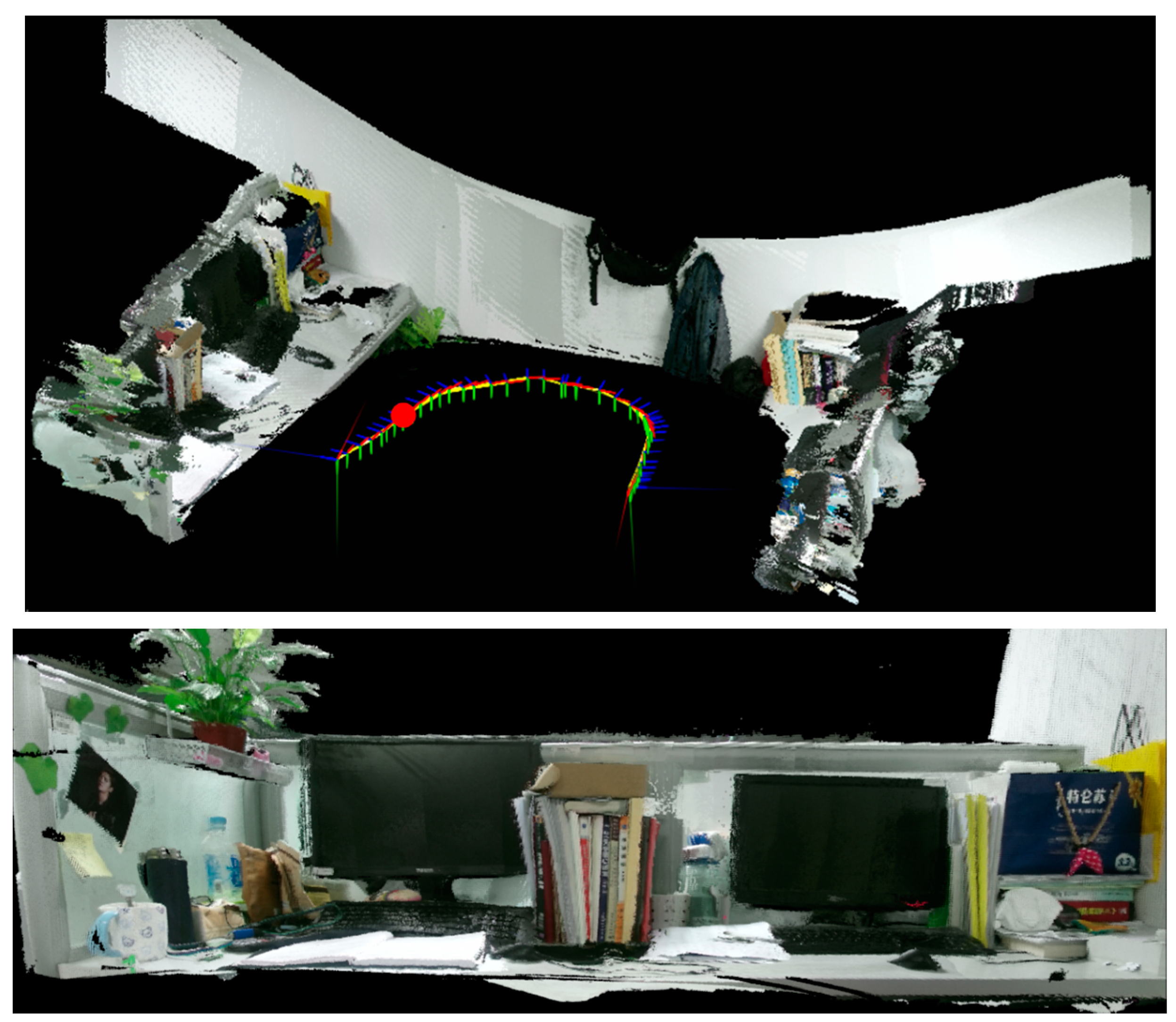
Figure 11.
A point cloud of the GMU Kitchen Dataset before (top) and after (bottom) correction using the post-rectification approach.
Figure 11.
A point cloud of the GMU Kitchen Dataset before (top) and after (bottom) correction using the post-rectification approach.


Table 1.
Technical specifications of the Kinect v2.
| Color | Camera Resolution | 1920 × 1080 pixels |
| Framerate | 30 frames per second | |
| Depth | Camera Resolution | 512 × 424 pixels |
| Framerate | 30 frames per second | |
| Field of VIEW (depth) | Horizontal | 70 degrees |
| Vertical | 60 degrees | |
| Operative Measuring Range | from 0.5 m to 4.5 m | |
| Depth Technology | Time-of-flight (ToF) | |
| Tilt Motor | No | |
| USB Standard | 3.0 | |
Table 2.
The expectation of offset of six kinds of reflectivity at distance 1.4 m.
| Panel Level | Reflectivity |
|---|---|
| 0% | 0.9913 |
| 20% | 0.7981 |
| 40% | 0.6019 |
| 60% | 0.4125 |
| 80% | 0.1994 |
| 100% | 0.0011 |
Table 3.
Error sources for depth sensor of the Kinect v1 and Kinect v2 (√ represents yes, and × represents no).
Table 3.
Error sources for depth sensor of the Kinect v1 and Kinect v2 (√ represents yes, and × represents no).
| Depth Sensor | Kinect v1 | Kinect v2 | |
|---|---|---|---|
| Error Source | |||
| Ambient Background Light [7] | √ | √ | |
| Temperature Drift [19] | √ | √ | |
| Systematic Distance Error [19] | √ | √ | |
| Depth Inhomogeneity [7] | √ | √ | |
| Multi-Path Effects [20] | √ | √ | |
| Intensity-Related Distance Error [7] | × | √ | |
| Semitransparent and Scattering Media [20] | √ | √ | |
| Dynamic Scenery [20] | √ | √ | |
| Flying Pixel [7] | × | √ | |
Table 4.
Expectation and standard deviation of correction and uncorrection at different reflectivity.
Table 4.
Expectation and standard deviation of correction and uncorrection at different reflectivity.
| Distance (m) | 0.75 | 0.90 | 1.05 | 1.20 | 1.35 | 1.50 | 1.65 | 1.80 | 1.95 | 2.10 | ||
|---|---|---|---|---|---|---|---|---|---|---|---|---|
| Value (mm) | ||||||||||||
| Item | ||||||||||||
| 100% black | ||||||||||||
| mcorr | 0.1607 | −0.4710 | 0.6894 | −0.2793 | −0.5033 | 1.0029 | −1.5421 | 1.1476 | −0.7082 | −0.0217 | ||
| Scorr | 2.0669 | 2.3116 | 2.4457 | 2.4295 | 3.2557 | 3.1760 | 3.9849 | 3.6780 | 5.1154 | 4.4273 | ||
| m | 127.6166 | 123.7936 | 122.8260 | 114.3370 | 111.3207 | 119.5455 | 121.4907 | 123.1732 | 124.5892 | 129.7157 | ||
| s | 2.0669 | 2.3116 | 2.4457 | 2.4295 | 3.2557 | 3.1760 | 3.9849 | 3.6780 | 5.1154 | 4.4273 | ||
| 80% black | ||||||||||||
| mcorr | 0.0873 | −0.3563 | 0.4352 | −0.0085 | −0.7791 | 1.2867 | −1.5841 | 1.4674 | −0.6622 | 0.2705 | ||
| Scorr | 1.0963 | 1.3948 | 1.3684 | 1.5997 | 1.9776 | 2.3625 | 2.1146 | 1.8148 | 2.0750 | 3.4419 | ||
| m | 125.5293 | 121.8862 | 120.5257 | 112.3133 | 109.1780 | 118.3241 | 119.2202 | 121.5227 | 123.9722 | 127.9327 | ||
| s | 1.0963 | 1.3948 | 1.3684 | 1.5997 | 1.9776 | 2.3625 | 2.1146 | 1.8148 | 2.0750 | 3.4419 | ||
| 60% black | ||||||||||||
| mcorr | 0.3129 | −0.6364 | 1.1514 | −0.6131 | −0.3607 | 1.0400 | −1.9007 | 1.4719 | −1.0410 | −0.0744 | ||
| Scorr | 1.2006 | 1.3411 | 1.4766 | 1.1424 | 1.4639 | 1.7628 | 1.9563 | 1.6953 | 1.7913 | 2.2094 | ||
| m | 124.6040 | 121.4815 | 120.6797 | 111.3145 | 109.1095 | 116.9787 | 118.4527 | 121.9892 | 123.6846 | 128.0617 | ||
| s | 1.2006 | 1.3411 | 1.4766 | 1.1424 | 1.4639 | 1.7628 | 1.9563 | 1.6953 | 1.7913 | 2.2094 | ||
| 40% black | ||||||||||||
| mcorr | 0.0478 | −0.0596 | 0.1218 | 0.0904 | −0.4571 | 0.6311 | −0.8309 | 0.6094 | −0.4894 | −0.0280 | ||
| Scorr | 1.4408 | 1.7909 | 1.4628 | 1.4888 | 1.2835 | 1.5967 | 1.2283 | 1.3882 | 2.8126 | 1.6514 | ||
| m | 122.3192 | 120.1545 | 117.1464 | 109.2976 | 107.1321 | 114.7480 | 116.7984 | 119.2528 | 123.7405 | 125.8464 | ||
| s | 1.4408 | 1.7909 | 1.4628 | 1.4888 | 1.2835 | 1.5967 | 1.2283 | 1.3882 | 2.8126 | 1.6514 | ||
| 20% black | ||||||||||||
| mcorr | 0.1038 | −0.7496 | 0.9256 | −0.5031 | −0.2778 | 1.0179 | −1.3685 | 1.6489 | −0.4917 | 0.4327 | ||
| Scorr | 1.3713 | 1.6607 | 1.6392 | 1.4375 | 1.5381 | 1.8762 | 1.4057 | 1.2839 | 1.4366 | 2.5210 | ||
| m | 120.0186 | 116.1750 | 116.2189 | 108.1833 | 106.1495 | 113.9487 | 115.8037 | 118.9490 | 121.4179 | 125.7333 | ||
| s | 1.3713 | 1.6607 | 1.6392 | 1.4375 | 1.5381 | 1.8762 | 1.4057 | 1.2839 | 1.4366 | 2.5210 | ||
| 0% black (100% white) | ||||||||||||
| mcorr | 0.6980 | 0.0054 | 1.3 | 0.3592 | −0.0831 | 1.8191 | −1.0919 | 2.2539 | −0.2420 | 0.7992 | ||
| Scorr | 1.6839 | 1.8881 | 1.7393 | 1.6467 | 1.7178 | 2.0895 | 1.3940 | 1.1620 | 1.4396 | 2.6236 | ||
| m | 117.5105 | 113.7644 | 113.7520 | 105.6693 | 103.2963 | 112.9783 | 114.3643 | 117.4583 | 120.2713 | 124.4468 | ||
| s | 1.6839 | 1.8881 | 1.7393 | 1.6467 | 1.7178 | 2.0895 | 1.3940 | 1.1620 | 1.4396 | 2.6236 | ||
Table 5.
Parameters from the calibration of the Kinect v2 (by rounding).
| Camera | Intrinsic Parameters | ||||
| fx (mm) | fy (mm) | u0 (pixel) | v0 (pixel) | ||
| Color | 1144.361 | 1147.337 | 966.359 | 548.038 | |
| IR | 388.198 | 389.033 | 253.270 | 213.934 | |
| Camera | Distortion Coefficients | ||||
| k1 | k2 | k3 | p1 | p2 | |
| Color | 0.108 | −0.125 | 0.062 | −0.001 | −0.003 |
| IR | 0.126 | −0.329 | 0.111 | −0.001 | −0.002 |
| DepthShift (mm) | |||||
| IR | 60.358 | ||||
| Rotation Matrix | Translation Vector | ||||
| Color and IR | |||||
Table 6.
The expectation of offset of six kinds of reflectivity at distance 1.4 m.
| Reflectivity | 0.9913 | 0.7981 | 0.6019 | 0.4125 | 0.1994 | 0.0011 | |
| Expectation (mm) | |||||||
| m | 107.3987 | 109.0536 | 109.8727 | 112.3605 | 113.0718 | 115.2330 | |
© 2017 by the authors. Licensee MDPI, Basel, Switzerland. This article is an open access article distributed under the terms and conditions of the Creative Commons Attribution (CC BY) license (http://creativecommons.org/licenses/by/4.0/).
Share and Cite
MDPI and ACS Style
Jiao, J.; Yuan, L.; Tang, W.; Deng, Z.; Wu, Q. A Post-Rectification Approach of Depth Images of Kinect v2 for 3D Reconstruction of Indoor Scenes. ISPRS Int. J. Geo-Inf. 2017, 6, 349. https://doi.org/10.3390/ijgi6110349
AMA Style
Jiao J, Yuan L, Tang W, Deng Z, Wu Q. A Post-Rectification Approach of Depth Images of Kinect v2 for 3D Reconstruction of Indoor Scenes. ISPRS International Journal of Geo-Information. 2017; 6(11):349. https://doi.org/10.3390/ijgi6110349
Chicago/Turabian StyleJiao, Jichao, Libin Yuan, Weihua Tang, Zhongliang Deng, and Qi Wu. 2017. "A Post-Rectification Approach of Depth Images of Kinect v2 for 3D Reconstruction of Indoor Scenes" ISPRS International Journal of Geo-Information 6, no. 11: 349. https://doi.org/10.3390/ijgi6110349
Note that from the first issue of 2016, this journal uses article numbers instead of page numbers. See further details here.