Article

Relationship between MRPV Model Parameters from MISRL2 Land Surface Product and Land Covers: A Case Study within Mainland Spain

by
Patricia Arrogante-Funes
1,*,
Carlos J. Novillo
1,
Raúl Romero-Calcerrada
2,
René Vázquez-Jiménez
1,3 and
Rocío N. Ramos-Bernal
1,3
1
Departamento de Tecnología Química y Energética, Tecnología Química y Ambiental y Tecnología Mecánica, Universidad Rey Juan Carlos, C/Tulipán s/n, 28933 Móstoles, Madrid, Spain
2
Geography Group, Departamento de Ciencias de la Educación, Lenguaje, Cultura y Artes, Ciencias Histórica-Jurídicas y Humanísticas y Lenguas Modernas, Facultad de Ciencias Jurídicas y Sociales, Universidad Rey Juan Carlos, Paseo de los Artilleros s/n, 28032 Vicálvaro, Madrid, Spain
3
Cuerpo Académico UAGro CA-93 Riesgos Naturales y Geotecnología, Universidad Autónoma de Guerrero, Av/Lázaro Cárdenas s/n, CU, Chilpancingo 39070, Guerrero, Mexico
*
Author to whom correspondence should be addressed.
ISPRS Int. J. Geo-Inf. 2017, 6(11), 353; https://doi.org/10.3390/ijgi6110353
Submission received: 4 September 2017 / Revised: 2 November 2017 / Accepted: 4 November 2017 / Published: 10 November 2017

Abstract

:
In this study, we showed that the multi-angle satellite remote sensing product, MISR L2 Land Surface (MIL2ASLS), which has a scale of 1.1 km, could be suitable for improving land-cover studies. Using seven images from this product, captured by the multi-angle imaging spectroradiometer sensor (MISR), we explored the values reached by the three parameters (ρ0, Θ, and k) of the Rahman–Pinty–Verstraete model, which was modified by Martonchick (MRPV). Thereafter, we compared the values and behaviors shown in seven Co-ordination of Information on the Environment (CORINE) land cover categories, in the red and near infrared (NIR) bands, over the seven MISR orbits captured in 2006 for Mainland Spain. Furthermore, we used Normalized Difference Vegetation Index (NDVI), Leaf Area Index (LAI), and Fraction of Photosynthetically Active Radiation (FPAR) ancillary data and the illumination angles from the same pixels, which made up the images. These ancillary data were also provided by the MISR products. An inferential statistic test was performed to evaluate the relationship between each parameter–band combination, and the land cover in every MISR orbit used. The results suggested that the ρ0 parameters of this product seemed to be the most related to photosynthetic activity, and it should be comparable with the widely-used NDVI. On the other hand, the k and Θ parameter values were not related, or at least not entirely related, to the phenology of land coverage. These seemed to be more influenced by the anisotropy behavior of the studied land cover pixels. Additionally, we observed, by constructing analysis of variance, how the mean of each MRPV parameter–band differed statistically (p < 0.01) by land covers and orbits. This study suggested that the MISR MRPV model parameter data product has great potential to be used to improve land cover applications.

1. Introduction

For many years now, there has been a need to retrieve both spatial and vertical structural information from remote sensing in order to provide critical inputs for ecosystem and process models [1]. Descriptions of canopy structure are vital to obtain accurate radiative transfer modeling joined to water and energy balances, which are usually a poorly-modeled element of global ecosystem models [2]. Currently, remote sensing is the only realistic way to quickly obtain land surface information across wide regions and with a broad range of temporal scenes. Traditionally, sources of remote sensing that have been used the most have been multispectral signatures. However, non-photosynthetic canopy elements represent major biomass components, and the vertical distribution and structural density can vary extensively under canopies with similar multispectral signatures [3].
Quantitative description of vegetation structure has been proposed as one of the key requirements for a significant improvement in modeling the carbon cycle and global land characterizations [4]. The use of multi-spectral data, acquired during the growing season, is the most commonly-used approach for mapping vegetation and land cover. However, this method is usually limited, as it is only capable of indirectly capturing canopy height [4]. Therefore, active remote sensing technology, such is airborne Light Detection and Ranging (LiDAR) sensors , or the Geoscience Laser Altimeter System (GLAS) in satellite platforms are nowadays popular techniques for examining the structure of vegetation canopies. In this sense, there are several studies based on these techniques, and on different areas around the Earth, and within various fields of work. For instance, there exist studies that prove the utility of LiDAR metrics for modeling biomass and improving forest inventories [5,6,7], or their use to estimate urban tree damage in an individual tree estimation approach [8], or even to study plant phenotyping in the agricultural field [9]. There are also examples where researchers have fused LiDAR acquisitions with radar or spectral images. One of these is described in Reference [10], where the authors mapped and estimated forest area and aboveground biomass in the “Miombo Woodlands” in Tanzania using data from airborne laser scanning (ALS), interferometric synthetic aperture radar (InSAR) derived from TanDEM-X, RapidEye optical imagery, and global forest map products derived from Landsat and ALOS PALSAR L-band radar imagery, which yielded improvements in terms of precision in the estimations. However, the high cost of airborne LiDAR data collection over large areas ensures that much of the terrestrial Earth surface will not be covered by airborne acquisitions in the near future, and also makes it difficult for easy regular updates. Although LiDAR in a satellite platform could be a solution, it still cannot provide comprehensive spatially-contiguous LiDAR datasets. Some studies have demonstrated the utility of multiangular reflectance data for mapping vegetation structural characteristics [4,11,12,13]. The multiangular approach could provide potential in forest height mapping over large regions at a lower cost than LiDAR technologies, thereby allowing for more regular updates.
From the first data obtained by a satellite in the 1970s, it was possible to evaluate the fact that the reflectance of different land covers was dependent on observation and illumination angles. That dependence implied that land covers were not isotropic; that is, they did not reflect the same amount of energy in all directions. Therefore, the source of noise must be corrected [14]. In those years, the Bidirectional Reflectance Function (BRDF) was defined as a variable that explained that reflectance was dependent on both the observation and illumination angles, as well as the wavelength of reflected radiation [5]. However, it was also possible to verify how magnitude and contour of this function expressed land cover composition, shape, and geometric structure where the incident energy was reflected [5].
Next, the anisotropy that the different terrestrial surfaces presented were considered as the noise to correct, or as an opportunity to explore land surface 3D characteristics. For the study of the land covers anisotropy, the launch of satellites with onboard sensors was promoted. These sensors allowed the study of different directional behaviors when a target reflected solar radiation. Out of these sensors, it is important to name the POlarization and Directionality of the Earth’s Reflectances instrument (POL-DER), the Multi-angle Imaging SpectroRadiometer (MISR), and the Compact High-Resolution Imaging Spectrometer (CHRIS Proba). The latter two have the ability to capture images of almost the same location (pixel) from several different angles during the same flight path [15]. In this sense, it was easy to find several studies where MISR products were used. Recently, different authors (e.g., References [15,16,17,18,19,20,21]) have proven the MISR utility for characterizing vegetal canopy, and for mapping vegetation and land cover at medium- and large-spatial scales.
The effects of the anisotropic behavior of the different targets can be observed in all remote sensing data, but the magnitude of these effects changes with object reflection properties. Different radiative transfer models (RTM) have been developed to try and model BRDF effects of surfaces, depending on their features. Vegetation RTM describes the interaction of light and vegetal canopy by combining different view and illumination conditions with their structural and biochemical properties. Today, there are several RTM models, including the Rahman–Pinty–Verstraete model (RPV) [22]. MISR level 2 land product (MI2ASLS) provides the parameters for the modified RPV model (MRPV). It is a semi-empirical, multiplicative, three-parameter model that returns Bidirectional Reflectance Factor (BRF) values for an arbitrary geophysical medium [23,24]. Furthermore, the MRPV model parameters have been directly related to the density of trees, proportions of shadow and bright surfaces, anisotropic scattering, and solar zenith angles from the scenes taken [19,22,25,26,27,28,29,30].
Against this background, our objective was to study the values taken by three MRPV MISR L2 land surface parameters in the most representative seven agrarian and forest Co-ordination of Information on the Environment (CORINE) land cover categories in Mainland Spain (non-irrigated arable land, permanently irrigated band, agroforestry areas, broad-leaved forest, coniferous forest natural grasslands, and transitional woodland shrub) in the red and near infrared (NIR) spectral bands, and in various MISR schemes, captured in 2006 from Mainland Spain. Thereby, we sought to assess the relationship between the parameter values and land covers. This aim is considered crucial for future research, based on land cover studies in Mainland Spain through the use of the not-widely-studied product, MIL2ASLS, and its MRPV parameters.

2. Materials and Methods

2.1. Study Site

The study area for this research was the intersection of MISR path 200, 201, and Mainland Spain. This area starts in Block 56 and ends in Block 61 of MISR (see Figure 1). Mainland Spain has a wide range of different natural surfaces and is an example of the Mediterranean zone.

2.2. Co-Ordination of Information on the Environment Land Cover 2006

The CORINE (Co-ordination of Information on the Environment) Land Cover (CLC) consists of a set of maps of the European environmental landscape, based on photo-interpretation of satellite images (SPOT, Landsat TM, and The Multispectral Scanner System or better known MSS). Ancillary data (aerial photographs, topographic or vegetation maps, statistics, and local knowledge) were used to refine the interpretation and the assignment of the territory into the categories of CORINE Land Cover nomenclature. The smallest surfaces mapped were 25 hectares. Linear features less than 100 m in width were not considered [31].
The CORINE program provides comparable digital maps of land cover (and partly land use) for each country, and much of Europe. These maps shows 44 different land cover categories organized hierarchically in three levels [22].
We used a map from Spain that consisted of a 1:100,000 vectorial layer, from 2006. On that layer, seven CORINE land covers were studied (see Table 1). We selected these natural land cover categories, as we considered them, to be the most representative of our study area. Furthermore, they also represented different 3D structures and phenological characteristics, which are very important when considering if the three MRPV parameters from the MISR L2 land surface were somehow related to these land cover properties, as some authors have noted [10,13,16,17,18,19,20,21].

2.3. MISR and MISR Data Used

The Multi-angle Imaging Spectroradiometer (MISR) was launched on 18 December 1999, and has a sensor with a 705 km sun-synchronous Earth orbit, which is onboard the Earth Observing System (EOS) Terra spacecraft. The MISR instrument has nine push cameras that view the Earth’s surface from different angles (nominal and design values); 0° (An), 26.1° (Af, Aa), 45.6° (Bf, Ba), 60.0° (Cf, Ca), and 70.5° (Df, Da), relative to nadir. In both, (f) corresponds to forward and (a) is relative to afterward, along the direction of the flight. This sensor gathers Earth information in four spectral bands, positioned at 446, 558, 672, and 866 nm, with a temporal resolution from 2 to 9 days, and a spatial resolution of 1100 or 275 m [32].
The MISR team provides several elaborate data products, including MIL2ASLS. This product provides bi-hemispherical reflectance (BHR), hemispherical directional reflectance factor (HDRF), directional-hemispherical reflectance (DHR), bi-hemispherical reflectance (BHR), and the bidirectional reflectance factor (BRF). MIL2ASLS product also includes parameters for reflectance factors based on a semi-empirical modified MRPV model (ρ0, Θ, and k), Leaf Area Index (LAI), fraction of photosynthetically-active radiation (FPAR), and the normalized difference vegetation index (NDVI) [32]. MIL2ASLS shows a 1.1-km spatial resolution, and is provided without data in some locations. These no-data zones are a consequence of glitter contamination, topographical accidents, or the presence of clouds [33].
As mentioned in the Introduction, we worked with the three parameters (ρ0, Θ, and k) of the RPV model, which were modified by Martonchik et al. [29] (MRPV). In addition to these parameters, we used some ancillary data, also provided by the MIL2ASLS product. These auxiliary data consisted of NDVI, FPAR, LAI, and zenith and azimuth illumination angle measurements from the same MISR orbits as the MRPV parameters. The MISR dataset was from 2006, as the CORINE land cover map used here was for that year. We used seven MISR images, as we wanted to maximize the number of pixels without errors and clouds; moreover, these pixels must be the same along the dates. We also needed to ensure that at least one MISR image from every season was included in the dataset (see the MIL2ASLS MISR orbits used in Table 2 and Figure 1).

2.4. Rahman–Pinty–Verstraete Modified (MRPV) Model

Rahman et al. [22] introduced a nonlinear, empirical, three-parameter model for vegetation canopy, which is abbreviated as the RPV (Rahman–Pinty–Verstraete) model. The RPV model splits a BRF field into an amplitude component (ρ0). The BRF field is represented by the product of three separate functions, accounting for both the viewing and illumination directions. The RPV model formulates the BRF of a surface as:
ρsfc (z0, Ω0, → Ω; ρ0, ρc, Θ, k) = ρ0 MI0, θ; k) FHG (g; Θ) H (ρc; G),
where
M I   ( θ 0 ,   θ ;   k )   =   cos k 1 θ 0 cos k 1 θ ( cos θ 0 + cos θ ) 1 k ,
F HG   ( g :   Θ )   =   1 Θ 2 ( 1 + 2 Θ cos g + Θ 2 ) 3 / 2 ,
H   ( ρ c ;   G )   =   1   +   1 ρ c 1 + G ,
cos g = cos θ cos θ0 + sin θ sin θ0 cos ɸ,
G = [tan2 θ0 + tan2 θ0 – 2 tan θ0 tan θ cos ɸ]1/2
where ρ0 yields the overall reflectance level; and θ and θ0 are the observation and illumination zenith angles, respectively. The relative azimuth angle (ɸ) is zero when the source of illumination is behind the sensor. MI is the modified Minnaert function, which permits the mathematical representation of all shapes of the angular field through the k parameter. The k parameter represents bowl- (indicated by k < 1) or bell- (indicated by k > 1) shaped anisotropy. The function FHG is based on the Henyey–Greenstein function, and the parameter Θ establishes the degree of forward (positive Θ) or backward (negative Θ) scattering. The H function allows the modeling of a hotspot with the ρ0 parameter. In some cases, the parameter accounting for the hot spot effect, ρc, can be set at a fixed value or equaled to the scalar amplitude parameter ρ0, being three parameters instead of four. The MIL2ASLS product only includes three parameters (ρ0, k and Θ).
Martonchik et al. [20] modified the RPV model by replacing its Henyey–Greenstein function with an exponential function after applying a logarithmic transformation, which resulted in the MRPV quasi-linear model being obtained. The fact that it is a quasi-linear model makes it easier to use in an operational context [23,34].

2.5. Data Processing and Data Analysis

The MIL2ASLS data from the seven MISR schemes in the red and NIR band were downloaded from the NASA Langley Distributed Active Archive Center (DAAC) and re-projected from the Space Oblique Mercator (SOM) to the Universal Transverse Mercator (UTM) system. We worked with red and NIR bands as these have the wavelengths most related to natural land covers in the available MISR bands, and, for that reason, they are the most studied in the literature [35].
We observed cloud contamination in some pixels from the MIL2ASLS product; therefore, an additional cloud mask was applied on each of the seven MISR schemes. This cloud mask was created through RGB compositions, which, in turn, were constructed by the BRF values from the red channel of Da, An, and Df cameras of each of the study area pixels. These BRF values were obtained from the MI1B2T product, which can be downloaded from the same site as MIL2ASLS. In this manner, it was easy to detect cloud contamination pixels by eye, and were therefore easy to remove [36].
We also carried out a buffer of 500 m on the CORINE land cover map with the seven CLC categories shown in Table 1. The buffer operation was carried out to avoid mixing the two or more types (at least 78% homogeneity in the land cover category of every pixel) that could have different behaviors in their phenology or 3D structural properties, and may translate into noise in the parameter values of every MISR image.
Next, the center of the pixels of the three parameters (ρ0, Θ, and k) and the ancillary data (NDVI, FPAR, LAI, and zenith angles) obtained from the MIL2ASLS images were spatially joined with the CORINE land cover map that resulted after applying the buffer and selecting the categories. As a consequence of this operation, we obtained a composition map made up of points with the parameter, as well as the ancillary variable values, CLC code, MISR band, and orbit (date of capture) information from the study area. Then, we assessed the reliability pixel value included in MIL2ASLS. Finally, pixels were selected at random to obtain a sample made up of 30 different pixels from each MISR orbit and CLC category. The latter was created to have a balanced analysis to perform other inferential analyses with robust results using this kind of sample. It is important to note that some of the FPAR and LAI showed no data, as it is difficult to get a random sample with 30 data pixels for these two variables.
With the final sample of pixels, we built a box plot by grouping the variables by CLC 2006 codes and MISR orbits. Then, the Spearman correlation coefficients between each combination parameter–band were calculated, as well as the NDVI, FPAR, and LAI, in order to evaluate the relationship between the MRPV parameters of this MISR product and the variables that express the phenological character of land covers.
Finally, we constructed linear multi-regression models and the variance analysis (ANOVA) and Kruskal–Wallis test. The linear regression models were made using as dependent variable (Y) each parameter–band combination, and using the CLC category and orbit as explanatory variables (Xn). A two-factor test of variance (ANOVA and Kruskal-Wallis) was conducted, using each combination parameter band as a numerical variable, and in which the categorical variables were the CLC category and the MISR orbit. These tests were made first to assess the relationship between land cover and orbit and the values achieved by the parameters. On the other hand, variance tests were performed to evaluate how the parameter–band combination differed between land covers and/or between MISR orbits captured on different days and belonging to different seasons. We decided to apply ANOVA and the Kruskal Wallis test (the non-parametrical test of variance) as some analyses of variance did not meet the homoscedasticity assumption of the parametrical test. Finally we used a post hoc pairwise test (Tukey) to know what pairs of CLC categories or orbits were statistically different.

3. Results and Discussion

3.1. Rahman–Pinty–Verstraete Modified (MRPV) Model Parameters Behavior in Different Land Uses and Captures in Mainland Spain

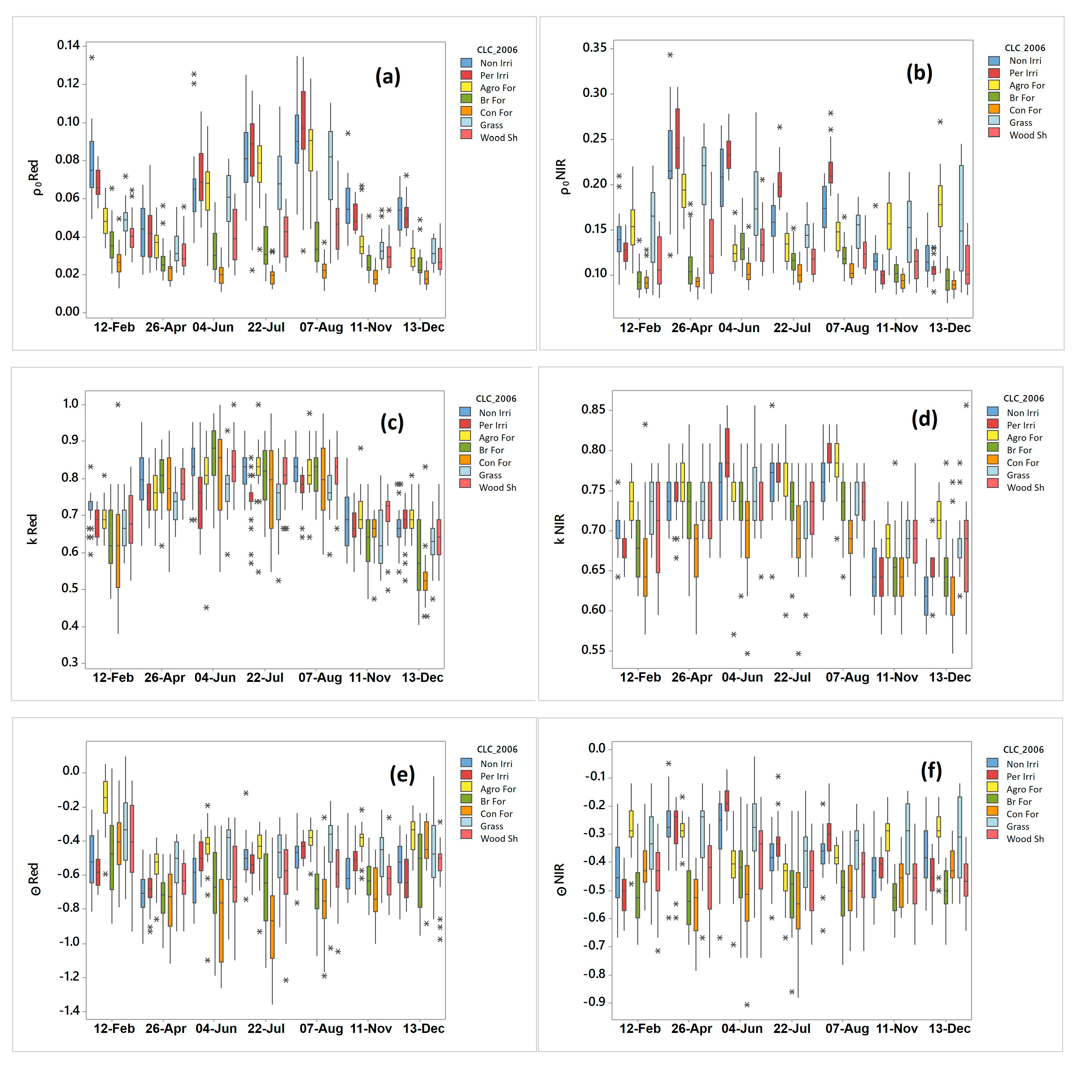
Figure 2 shows the ρ0, Θ and k values in the red and NIR spectral bands of MISR orbits from 2006 in different classes of land use CLC for Peninsular Spain.
The ρ0 red values from the MISR scenes ranged between 0.01 and 0.14, while those related to ρ0 NIR were between 0.05 and 0.35. Meanwhile, the k red average values were from 0.35 to 1, and, for the k NIR, oscillated between 0.5 and 0.9. Finally, the average values of Θ in the spectral band of red were between –0.1 and –1.4, and those found in the NIR band were from 0 and –0.9 (see Figure 2).
After reviewing the values presented by other authors (who have also worked with the parameters of the MRPV model), we verified that the values reported in our study coincided with those examined in the literature [25,37,38].
The graphs in Figure 2 show that the k values were never greater than one; furthermore, the Θ parameter values were always negative. The latter indicated a predominance of backscattering [26,37,38]. Pinty et al. [17] were the first to report how the anisotropic character of terrestrial targets is influenced by the structure and density of vegetation on a sub-pixel scale. The authors of the papers cited before demonstrated how, for a light soil with dark and vertical vegetation, the presence of trees at medium-high densities created a bell shape (values on the BRF curve along the viewing angles). This pattern was observed in the red spectrum, as in NIR, this spectral contrast between the bright background and the trees occurred on the contrary [17]. The k values less than one indicated how the BRF curve, along the zenith observation angles, presented a bowl shape, the most common in natural land covers overall, at a 1.1-km spatial resolution [26]. This parameter was highly dependent on spatial resolution, and when we have a medium resolution (as the MIL2ASLS product is), it appeared harder to find the bell form BRF curve [26], which occurred in our results.
On the one hand, Figure 2 shows how parameter ρ0, in the Br For, Con For, and Wood Sh CLC categories, presented more similar median values in all the MISR orbits than the other land cover classes. These results were consistent with those exposed by Alcaraz-Segura [39], who used NDVI values in the Iberian Ecosystems, instead of ρ0 ones. Figure 2 also shows how the average values from the Con For CLC were still more similar in the study of MISR orbits than values belonging to Br For, or even more so than those belonging to Wood Sh. This is because Con For on the CLC 2006 map is more homogenous than Br For CLC, which does not show separate deciduous and evergreen plants. The last point explains the fact that, in Figure 2a,b, we can observe ρ0 red and NIR values from Br For CLC with more dispersion within the same orbit (interquartile range found in the boxplots) than in Con For CLC. Additionally, this also explains the fact that we could see more steady behavior in the values of ρ0 red and NIR pixels belonging to the Br For and Wood Sh CLC categories.
In 
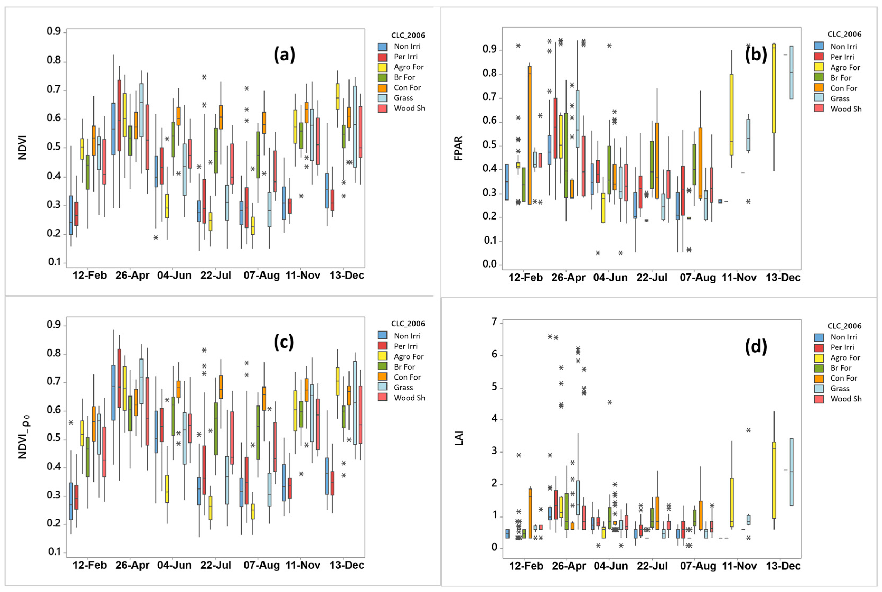
Figure 2a,b, it can be seen how the crops (Non Irri, Per Irri), pasture (Grass), and agroforestry (Agro For) CLC ρ0 red, as well as ρ0 at NIR values, presented more variability through the MISR orbits, taken on seven different dates, than the Br For, Con For and Wood Sh classes did. In general, the trend of the ρ0 red and NIR values seemed to be related to the land covers phenological pattern. To further investigate this idea, we focused on Figure 3, which shows four graphs with the NDVI, FPAR, NDVI calculated using the ρ0 red and NIR values (in Figure 2a,b) and the LAI variables. From Figure 3a,c, the median and the interquartile ranges were extracted, and, in general, the behavior of the ρ0 and NDVI values along the seven MISR orbits were quite similar. The FPAR (Figure 3b) and the LAI value (Figure 3d) dispersion within one CLC and orbit were higher than the dispersion taken using NDVI (Figure 3a) and NDVI from ρ0 (Figure 3c). However, the median values that demonstrated the behaviors of these four variables (Figure 3) were similar. Thereby, in general, it can be noted that the mean values may support the idea that the ρ0 parameter has a relationship with spectral properties and land cover phenological features, as other authors have already described [19,25].
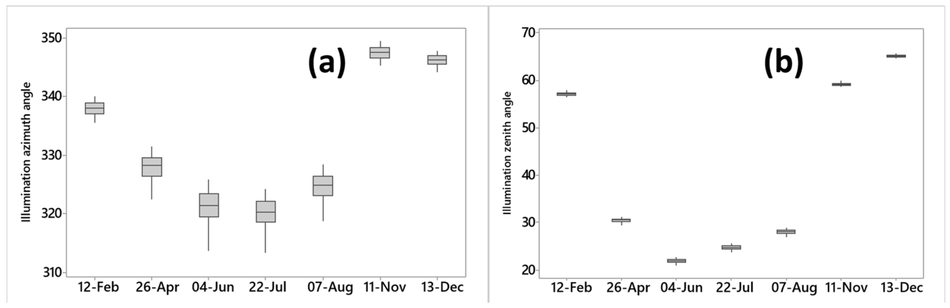
The k parameter in the NIR and the red band seemed to present lower median values in the orbits belonging to winter and autumn than in those of summer and spring (this fact was slightly more marked in the red wavelength than in the NIR one). That is to say, the covers present, in general terms and from the k parameter, a more isotropic behavior (k values close to the unity) from the dates in summer and spring than in those of autumn and winter. Furthermore, the zenith angles from the MISR scenes used here were higher in the winter images than in those belonging to summer and spring, as seen in Figure 4.
The parameter k shows the difference between observing BRF from the nadir camera in comparison to the BRF from other positions, further away from this nadir position [18,40]. The fact that finding average values of k expressed greater anisotropy in the winter and autumn schemes than in summer and spring indicated the influence of the zenith illumination angle on these values. That is, in winter, the sun position is farther from the zenith than in spring and summer. This fact also implied that, in winter and autumn, the sensor captured much more shade from the nadir in comparison with other positions more distant from it, than in summer and winter. Thereby, it could be found greater anisotropy expressed by k in winter and autumn than in summer and spring. The influence of the zenith angle of the data collection on the values reached by k has already been reported in Pinty et al. [17] or in Reference [37]; furthermore, their results coincided with those presented in our current work.
From Figure 3c,d, it can be seen that the k parameter values did not follow the same behavior as ρ0, NDVI, FPAR, and LAI, i.e., the values reached by k did not seem to be dependent on the phenology.
Figure 2e,f shows the Θ parameter pixel values in the different orbits and CLC categories used in this study. The Θ values given from the land use classes in the seven MISR orbits were more anisotropic in the red band than in the NIR, i.e., the values reached were lower in red than in NIR. This fact was due to the effect of multiple dispersion on the NIR channel, which caused the anisotropic behavior to be less than in the red band. This physical effect was observed and explained by Sandmeier et al. [32]. Furthermore, these results were consistent with those obtained by Armston et al. [19], where the authors studied different natural covers and dates in Queensland, Australia, and found this effect on bare soil, as well as in soil in addition to vegetation.
A comparison of these graphs (Figure 2e,f) to the NDVI, FPAR, and LAI ones (Figure 3) showed that the trends that followed the median and the interquartile ranges of each variable were not very similar. For instance, the Θ red and NIR values of the Grass CLC category appeared to be steadier through the orbits than the others. The Θ red values of the Br For CLC class were slightly more stable through the orbits than the values belonging to the Con For CLC category; however, the NDVI plot (Figure 3a) occurred on the contrary.
With regards to the anisotropy described by the Θ parameter in our study, it could be appreciated how the Br For and Con For CLC categories were those that presented Θ values more different than zero, i.e., they were the most anisotropic from the perspective of the Θ parameter. Camacho de Coca et al. [41] explained that the natural land covers made up of vegetation with a predominance of vertical structure 3D were the most anisotropic, and even more so when the background was bright. For that reason, it also explained why we found that the values of the Θ parameter were even more different than zero (more anisotropic) in the orbits used that belonged to summer or near summer. It is in those orbits where the background as the driest of all seven dates used for this study (see Figure 2e,f).

3.2. MRPV Model Parameters Related to NDVI, LAI, FPAR

Table 3, Table 4 and Table 5 show the Spearman Rho’s coefficient between the MRPV parameters from the MIL2ASLS and the NDVI, FPAR, and LAI. In the tables, no Rho’s coefficient value meant that the relationship was not significant. The results suggested that the correlation was stronger between the ρ0 and NDVI than between the other three parameters and the NDVI, as well as occurring cases in the correlation between these MRPV parameters and the FPAR and LAI variables. The correlation between ρ0 red and NDVI, FPAR and LAI was slightly stronger than that between the ρ0 NIR and NDVI, FPAR, and LAI. Finally, it appeared that the relationship between Θ and the last variables mentioned were higher than the relationship between those and the k parameter. These results proved (as seen in Figure 2 and Figure 3) the relationship between the ρ0 parameter and the NDVI, FPAR, and LAI, and matched those described by other authors using different sites than our study area [19,25].

3.3. Inferential Statistics

Table 6 shows the results of the linear model regressions and the parametric analyses of variance performed using the MRPV parameters (Y) and the categorical variables, named MISR orbit and CLC category (Xn). Table 7 presents the results from the non-parametric test of variance. At a glance, the results showed how the two categorical variables explained the parameters in a significant way (p < 0.01) (see Table 6). The models yielded adjusted R-square values, which rated between 0.37 and 0.74. Taking both the adjusted R-square and F statistics values into account, it appeared that the relationship between the parameters and the MISR dates and CLC category was stronger in the case of ρ0 than in the k, and was weakest in the models explaining the Θ parameter.
All analysis of variance performed showed significantly different mean and median using Orbit, CLC, and Orbit and CLC (see Table 6 and Table 7). The resulting F from the parametrically analyses of variance, as well as the Chi-square results from the non-parametrically analyses of variance (see Table 6 and Table 7) were higher for the CLC than for the MISR orbit factor in tests related to ρ0 and Θ, and was the opposite in the case of the k parameter test. The NDVI F and Chi-square values were similar between the CLC and Orbit cases.
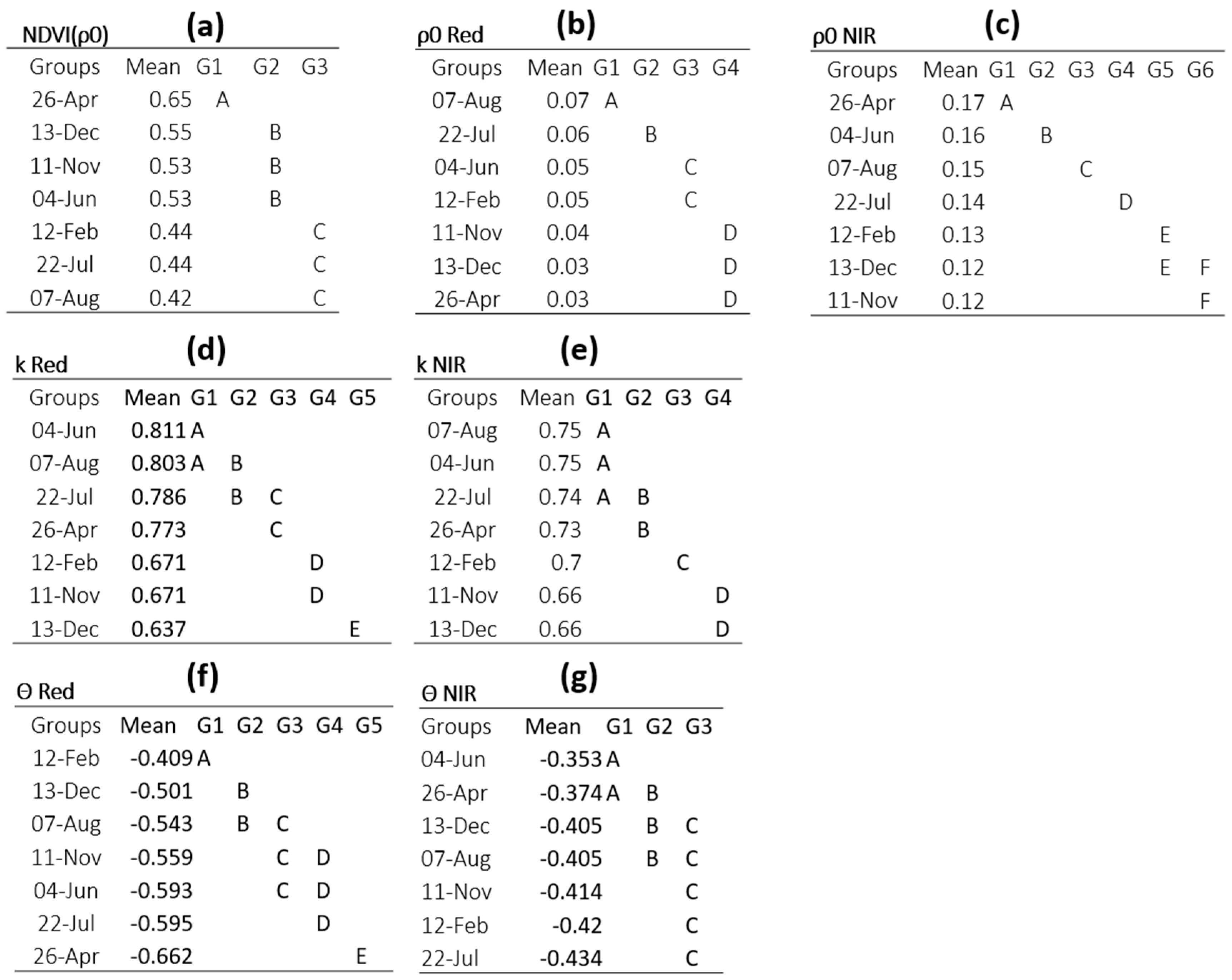
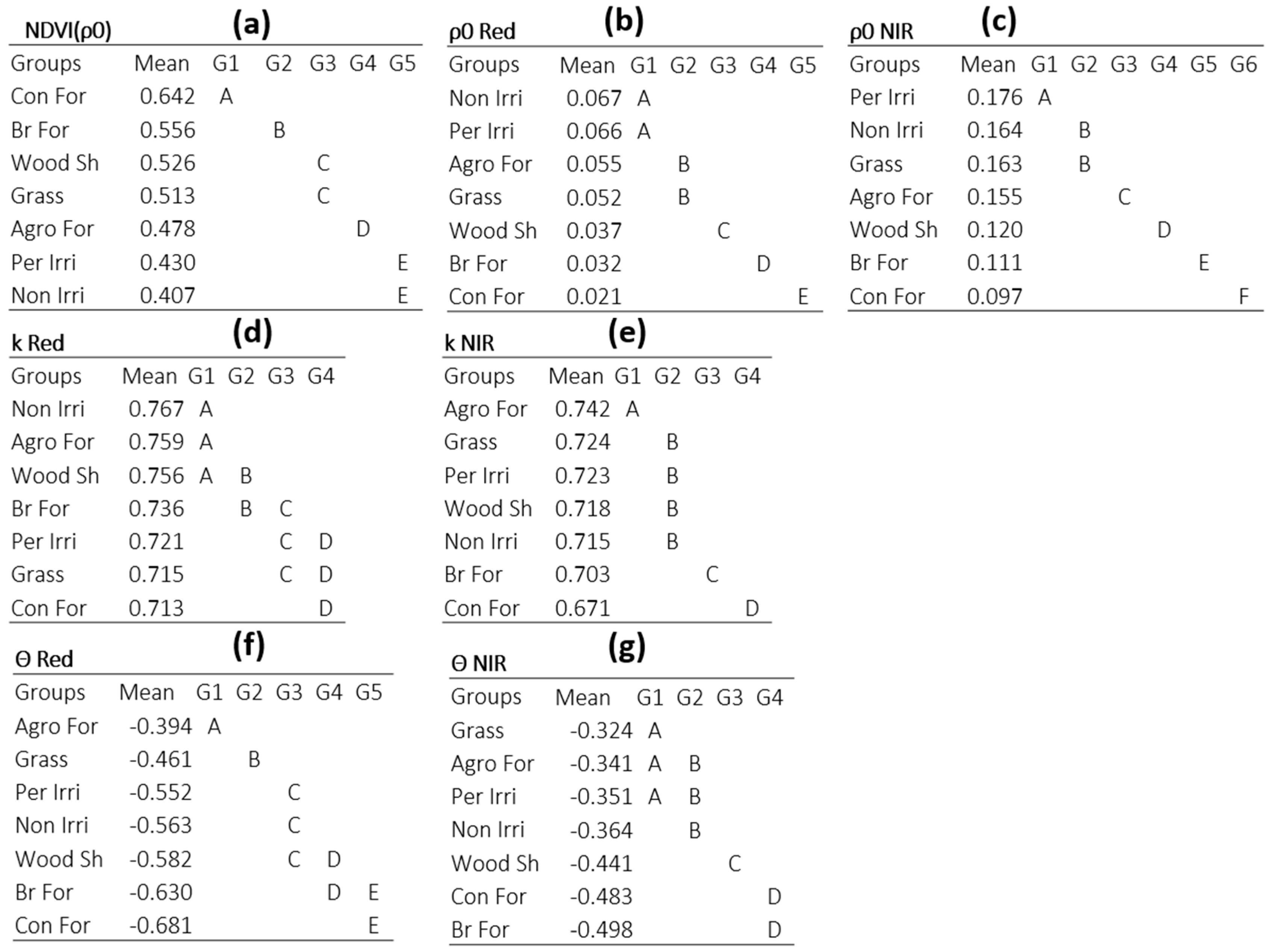
For the post hoc test performed using the CLC categories shown in Figure 5, the results illustrated that the majority of these groups were significantly different, using NDVI (ρ0) mean values. This was a good result, since the aim was to use this parameter, for instance, to separate between land covers, but was not a striking finding, as NDVI has already been utilized in some studies [35] to classify or to detect changes in the land uses. For this reason, we focused on the pair of images that did not significantly differ from the mean NDVI (ρ0) values. These pairs were built using the Wood Sh and the Grass (transitional woodland-shrub and natural grassland), and the pair formed by the Non Irri and Per Irri (non-irrigated arable land and permanently irrigated arable land) CLC categories. Table 7 shows, on the one hand, that the pair conformed by Wood Sh and Grass were significantly different from the mean values of the k red and NIR and by the Θ red and Θ NIR. On the other hand, the pair built by Non Irri and Per Irri differed statistically from the mean values of the k red. Thus, these results may indicate that the k and Θ parameters from the MIL2ASLS product, in addition to ρ0, which matched well with classical NDVI (like the results shown in Section 3.2), could help to differentiate between those land covers, which are difficult to differentiate with NDVI even, including data for different seasons of the year.
For the post hoc test performed using the MISR orbit (Figure 6a) it can be seen that the NDVI (ρ0) values were grouped into three categories. The first category was made up of the MISR orbit from April, which presented the highest mean value, the other was made up of the orbits from December, November, and June. Finally, the last category was confirmed by the orbits of February, July, and August which showed the lowest value of NDVI (ρ0). Effectively, the vegetation in those three categories, in general, presented very marked different phenological behaviors within Mainland Spain. However, for the k and the Θ parameter, the classes resulting from the post hoc test were not conformed in the same way as in the NDVI (ρ0).
In general, the parameter-band CLC categories in the different studied orbits had a high degree of separability, at least given that the mean values belonged to its CLC or orbit. This is why other authors have included multi-angular information in their work on the classification of images, among other utilities. For example, Brown et al. [42] observed how the inclusion of multi-angular information, in addition to only multi-spectral from the POLDER sensor, produced an improvement in the overall accuracy of close to five percent, achieving a maximum improvement between the classes of wooded savanna and grassland. On the other hand, Mahtab et al. [43] also obtained increases in the degree of separability of classes, introducing multi angular information in addition to multispectral. Su et al. [44] increased the overall accuracy by 10–15% using multi-angle information, which was also used to classify between different types of coverage. MIL2ASLS with its MRPV parameters provide us with a source of multi spectral and multi angular information that can be successfully used for great- and medium-scale land cover studies. This is because this product provides a multispectral view of classical remote sensing, thanks to the ρ0 parameter, and, on the other hand, a multi-angular view with the k and Θ parameters.

4. Conclusions

According to the results presented in the sections of this study, it can be said that the parameter ρ0 (at the red and NIR channel) seemed to be the most related to the NDVI, FPAR, and LAI, i.e., it appeared to be the parameter that could better express the photosynthetic activity or the phenological behavior in the land covers studied in Mainland Spain. We noted this first at a glance when comparing the boxplots of the ρ0 by CLC category in the different seven MISR orbits also captured on seven dates, with NDVI, FPAR, and LAI; and, second, by studying the Spearman correlation coefficient between the ρ0 and the other three variables. The k and the Θ parameter values (also at the red and NIR channel) from the pixels explored showed different patterns than those followed by NDVI, FPAR, and LAI. We compared the k and Θ with the illumination angles and noted how these angles could control, or at least somehow influence the values reached by the k and Θ parameters, and, therefore, the grade of anisotropy expressed by them.
From the inferential test, linear models were constructed to explain each combination of parameter and band, and their analyses of variance were executed using the CLC category and the MISR orbit as a categorical variable to allow us to assess how these two explicative variables could explain each parameter variance in a significant way. The CLC and the Orbit explained more variance of ρ0 than k or Θ, and post hoc tests, performed by pair groups, of these two variables, showed how ρ0, in general, alone or used as the classic NDVI form, showed many differences from its mean values. However, the key was to use ρ0 in addition to k or Θ, to assure the separability of the CLC types that could only not be differenced with ρ0.
This study suggested that, although the number of studies up to the present, used for the MIL2ASLS MRPV model parameter data product, is not very large, it has great potential to be used for improving land cover research. For this reason, amplifying the number of future studies and applications, which involve the parameters of MIL2ASLS, is worthwhile.

Acknowledgments

We acknowledge the comments by the anonymous referees that helped us to improve the paper. We would also like to thank the National Aeronautics and Space Administration, and the Copernicus Land Monitoring Service for images and data provided.

Author Contributions

Patricia Arrogante-Funes and Carlos J. Novillo conceived and designed the experiments; Patricia Arrogante-Funes performed the experiments; Patricia Arrogante-Funes, Carlos J. Novillo, Raúl Romero-Calcerrada, René Vázquez-Jímenez y R.N. Ramos-Bernal analyzed the data, wrote parts, revised and improved the proposed article.

Conflicts of Interest

The authors declare no conflict of interest.

References

  1. Hill, M.J.; Averill, C.; Jiao, Z.; Schaaf, C.B.; Armston, J.D. Relationship of MISR RPV parameters and MODIS BRDF shape indicators to surface vegetation patterns in an Australian Tropical Savanna. Can. J. Remote Sens. 2008, 34, S247–S267. [Google Scholar] [CrossRef]
  2. Morales, M.B.; Garcia, J.T.; Arroyo, B. Can landscape composition changes predict spatial and annual variation of little bustard male abundance? Anim. Conserv. 2005, 8, 167–174. [Google Scholar] [CrossRef]
  3. Lu, D.S.; Ge, H.L.; He, S.Z.; Xu, A.J.; Zhou, G.M.; Du, H.Q. Pixel-based Minnaert correction method for reducing topographic effects on a Landsat 7 ETM+ image. Photogramm. Eng. Remote Sens. 2008, 74, 1343–1350. [Google Scholar]
  4. Chopping, M.; Moisen, G.G.; Su, L.; Laliberte, A.; Rango, A.; Martonchik, J.V.; Peters, D.P.C. Large area mapping of southwestern forest crown cover, canopy height, and biomass using the NASA Multi-angle Imaging Spectro-Radiometer. Remote Sens. Environ. 2008, 112, 2051–2063. [Google Scholar] [CrossRef]
  5. Popescu, S.C.; Zhao, K.; Neuenschwander, A.; Lin, C. Satellite Lidar vs. Small footprint airborne Lidar: Comparing the accuracy of aboveground biomass estimates and forest structure metrics at footprint level. Remote Sens. Environ. 2011, 115, 2786–2797. [Google Scholar] [CrossRef]
  6. McRoberts, R.E.; Næsset, E.; Gobakken, T.; Bollandsås, O.M. Indirect and direct estimation of forest biomass change using forest inventory and airborne laser scanning data. Remote Sens. Environ. 2015, 164, 36–42. [Google Scholar] [CrossRef]
  7. Li, A.; Dhakal, S.; Glenn, N.; Spaete, L.; Shinneman, D.; Pilliod, D.; Arkle, R.; McIlroy, S. Lidar aboveground vegetation biomass estimates in shrublands: Prediction, uncertainties and application to coarser scales. Remote Sens. 2017, 9, 903. [Google Scholar] [CrossRef]
  8. Rahman, M.T.; Rashed, T. Urban tree damage estimation using airborne laser scanner data and geographic information systems: An example from 2007 Oklahoma ice storm. Urban For. Urban Green. 2015, 14, 562–572. [Google Scholar] [CrossRef]
  9. Sun, S.; Li, C.; Paterson, A. In-field high-throughput phenotyping of cotton plant height using Lidar. Remote Sens. 2017, 9, 377. [Google Scholar] [CrossRef]
  10. Næsset, E.; Ørka, H.O.; Solberg, S.; Bollandsåsa, O.M.; Hansen, E.H.; Mauya, E.; Zahabu, E.; Malimbwi, R.; Chamuya, N.; Olsson, H.; et al. Mapping and estimating forest area and aboveground biomass in miombo woodlands in Tanzania using data from airborne laser scanning, tandem-x, Rapideye, and global forest maps: A comparison of estimated precision. Remote Sens. Environ. 2016, 175, 282–300. [Google Scholar] [CrossRef]
  11. Chopping, M.; Nolin, A.; Moisen, G.G.; Martonchik, J.V.; Bull, M. Forest canopy height from the Multi-angle Imaging Spectroradiometer (MISR) assessed with high resolution discrete return Lidar. Remote Sens. Environ. 2009, 113, 2172–2185. [Google Scholar] [CrossRef]
  12. Chopping, M.; Schaaf, C.B.; Zhao, F.; Wang, Z.; Nolin, A.W.; Moisen, G.G.; Martonchik, J.V.; Bull, M. Forest structure and aboveground biomass in the southwestern united states from MODIS and MISR. Remote Sens. Environ. 2011, 115, 2943–2953. [Google Scholar] [CrossRef]
  13. Heiskanen, J. Estimating aboveground tree biomass and leaf area index in a mountain birch forest using Aster Satellite data. Int. J. Remote Sens. 2006, 27, 1135–1158. [Google Scholar] [CrossRef]
  14. Nicodemus, F.E.; Richmond, J.C.; Hsia, J.J.; Ginsberg, I.W.; Limperis, T. Geometrical considerations and nomenclature for reflectance. In Radiometry; Jones and Bartlett Publishers Inc.: Boston, MA, USA, 1992; pp. 94–145. [Google Scholar]
  15. Diner, D.J.; Braswell, B.H.; Davies, R.; Gobron, N.; Hu, J.; Jin, Y.; Kahn, R.A.; Knyazikhin, Y.; Loeb, N.; Muller, J.-P.; et al. The value of Multi-angle measurements for retrieving structurally and radiatively consistent properties of clouds, aerosols, and surfaces. Remote Sens. Environ. 2005, 97, 495–518. [Google Scholar] [CrossRef]
  16. Gobron, N.; Pinty, B.; Verstraete, M.M.; Widlowski, J.-L.; Diner, D.J. Uniqueness of Multi-angular measurements. II. Joint retrieval of vegetation structure and photosynthetic activity from MISR uniqueness of multia-ngular measurements. II. Joint retrieval of vegetation structure and photosynthetic activity from MISR. IEEE Trans. Geosci. Remote Sens. 2002, 40, 1574–1592. [Google Scholar] [CrossRef]
  17. Zhang, Y.; Tian, Y.; Myneni, R.B.; Knyazikhin, Y.; Woodcock, C.E. Assessing the information content of multi-angle satellite data for mapping biomes: I. Statistical analysis. Remote Sens. Environ. 2002, 80, 418–434. [Google Scholar] [CrossRef]
  18. Nolin, A.W. Towards retrieval of forest cover density over snow from the Multi-angle Imaging Spectroradiometer (MISR). Hydrol. Process. 2004, 18, 3623–3636. [Google Scholar] [CrossRef]
  19. Armston, J.D.; Scarth, P.F.; Phinn, S.R.; Danaher, T.J. Analysis of multi-date MISR measurements for forest and woodland communities, Queensland, Australia. Remote Sens. Environ. 2007, 107, 287–298. [Google Scholar] [CrossRef]
  20. Su, L. Optimizing support vector machine learning for semi-arid vegetation mapping by using clustering analysis. ISPRS J. Photogramm. Remote Sens. 2009, 64, 407–413. [Google Scholar] [CrossRef]
  21. Selkowitz, D.J. A comparison of multi-spectral, multi-angular, and multi-temporal remote sensing datasets for fractional shrub canopy mapping in arctic Alaska. Remote Sens. Environ. 2010, 114, 1338–1352. [Google Scholar] [CrossRef]
  22. Rahman, H.; Pinty, B.; Verstraete, M.M. Coupled surface-atmosphere reflectance (CSAR) model 2. Semi-empirical surface model usable with NOAA advanced very high-resolution radiometer data. J. Geophys. Res. 1993, 98, 20791–20801. [Google Scholar] [CrossRef]
  23. Diner, D.J.; Asner, G.P.; Davies, R.; Knyazikhin, Y.; Muller, J.P.; Nolin, A.W.; Pinty, B.; Schaaf, C.B.; Stroeve, J. New directions in earth observing: Scientific applications of multi-angle remote sensing. Bull. Am. Meteorol. Soc. 1999, 80, 2209–2228. [Google Scholar] [CrossRef]
  24. Engelsen, O.; Pinty, B.; Verstraete, M.M.; Martonchik, J. Parametric Bidirectional Reflectance Factor Models: Evaluation, Improvements and Applications; Office for Official Publications of the European Communities: Ispra, Italy, 1996. [Google Scholar]
  25. Lavergne, T.; Kaminski, T.; Pinty, B.; Taberner, M.; Gobron, N.; Verstraete, M.M.; Vossbeck, M.; Widlowski, J.-L.; Giering, R. Application to MISRl and products of an RPV model inversion package using adjoint and hessian codes. Remote Sens. Environ. 2007, 107, 362–375. [Google Scholar] [CrossRef]
  26. Pinty, B.; Widlowski, J.L.; Gobron, N.; Verstraete, M.M.; Diner, D.J. Uniqueness of Multi-angular measurements. I. An indicator of subpixel surface heterogeneity from MISR. IEEE Trans. Geosci. Remote Sens. 2002, 40, 1560–1573. [Google Scholar] [CrossRef]
  27. Widlowski, J.L.; Pinty, B.; Gobron, N.; Verstraete, M.M.; Davis, A.B. Characterization of surface heterogeneity detected at the MISR/TERRA subpixel scale. Geophys. Res. Lett. 2001, 28, 4639–4642. [Google Scholar] [CrossRef]
  28. Lucas, N.S.; Curran, P.J.; Plummer, S.E.; Danson, F.M. Estimating the stem carbon production of a coniferous forest using an ecosystem simulation model driven by the remotely sensed red edge. Int. J. Remote Sens. 2000, 21, 619–631. [Google Scholar] [CrossRef]
  29. Martonchik, J.V.; Diner, D.J.; Pinty, B.; Verstraete, M.M.; Myneni, R.B.; Knyazikhin, Y.; Gordon, H.R. Determination of land and ocean reflective, radiative, and biophysical properties using multi-angle imaging. IEEE Trans. Geosci. Remote Sens. 1998, 36, 1266–1281. [Google Scholar] [CrossRef]
  30. Schaaf, C.; Strahler, A.; Gao, F.; Lucht, W.; Jin, Y.; Li, X.; Zhang, X.; Tsvetsinskaya, E.; Muller, J.P.; Lewis, P.; et al. Global Albedo, BRDF and Nadir BRDF-Adjusted Reflectance Products from MODIS. In Proceedings of the International Geoscience and Remote Sensing Symposium (IGARSS), Toronto, ON, Canada, 23–28 June 2002; pp. 1188–1190. [Google Scholar]
  31. European Environment Agency (EEA). Clc2006 Technical Guidelines; Technical Report No 17/2007; EEA: Copenhagen, Denmark, 2007. [Google Scholar]
  32. Diner, D.J.; Beckert, J.C.; Reilly, T.H.; Bruegge, C.J.; Conel, J.E.; Kahn, R.A.; Martonchik, J.V.; Ackerman, T.P.; Davies, R.; Gerstl, S.A.W.; et al. Multi-angle Imaging Spectroradiometer (MISR) instrument description and experiment overview. IEEE Trans. Geosci. Remote Sens. 1998, 36, 1072–1087. [Google Scholar] [CrossRef]
  33. Kokhanovsky, A.; de Leeuw, G.; Martonchik, J.; Kahn, R.; Diner, D. Retrieval of aerosol properties over land using MISR observations. In Satellite Aerosol Remote Sensing over Land; Springer: Berlin/Heidelberg, Germany, 2009; pp. 267–293. [Google Scholar]
  34. Martonchik, J.V.; Kahn, R.A.; Diner, D.J. Retrieval of Aerosol Properties over Land Using MISR Observations; Satellite Aerosol Remote Sensing over Land: Berlin, Germany, 2008. [Google Scholar]
  35. Chuvieco, E. Teledetección Ambiental: La Observación de la Tierra Desde el Espacio; Ariel Ciencia: Madrid, Spain, 2010. [Google Scholar]
  36. Novillo, C.J. Aplicaciones de Interés Forestal de las Imágenes Obtenidas con el Sensor Multi-Angle Imaging Spectroradiometer (MISR). Ph.D. Thesis, Universidad Politécnica, Madrid, Spain, 21 December 2012. [Google Scholar]
  37. Widlowski, J.L.; Pinty, B.; Gobron, N.; Verstraete, M.M.; Diner, D.J.; Davis, A.B. Canopy structure parameters derived from multi-angular remote sensing data for terrestrial carbon studies. Clim. Chang. 2004, 67, 403–415. [Google Scholar] [CrossRef]
  38. Biliouris, D.; van der Zande, D.; Verstraeten, W.; Stuckens, J.; Muys, B.; Dutré, P.; Coppin, P. RPV model parameters based on hyperspectral bidirectional reflectance measurements of Fagus sylvaticaL. Leaves. Remote Sens. 2009, 1, 92–106. [Google Scholar] [CrossRef]
  39. Alcaraz Segura, D. Caracterización del funcionamiento de los ecosistemas ibéricos mediante teledetección. Ecosistemas 2006, 15, 113–117. [Google Scholar]
  40. Pinty, B.; Gobron, N.; Widlowski, J.L.; Lavergne, T.; Verstraete, M.M. Synergy between 1-D and 3-D Radiation Transfer Models to retrieve vegetation canopy properties from remote sensing data. J. Geophys. Res. 2004, 109, D21205. [Google Scholar] [CrossRef]
  41. Camacho-de Coca, F.; García-Haro, F.J.; Gilabert, M.A. Quantitative analysis of the anisotropy of BRDF of land crops using airborne polder data. In Recent Advances in Quantitative Remote Sensing; Universidad de Valencia: Valencia, Spain, 2002; pp. 303–308. [Google Scholar]
  42. Brown, G.S.; Rettie, W.J.; Mallory, F.F. Application of a variance decomposition method to compare satellite and aerial inventory data: A tool for evaluating wildlife-habitat relationships. J. Appl. Ecol. 2006, 43, 173–184. [Google Scholar] [CrossRef]
  43. Mahtab, A.; Sridhar, V.N.; Navalgund, R.R. Impact of surface anisotropy on classification accuracy of selected vegetation classes: An evaluation using multidate multi-angular MISR data over parts of Madhya Pradesh, India. IEEE Trans. Geosci. Remote Sens. 2008, 46, 250–258. [Google Scholar] [CrossRef]
  44. Su, L.; Chopping, M.J.; Rango, A.; Martonchik, J.V.; Peters, D.P.C. Support vector machines for recognition of semi-arid vegetation types using MISR multi-angle imagery. Remote Sens. Environ. 2007, 107, 299–311. [Google Scholar] [CrossRef]
Figure 1. Examples of Multi-angle Imaging SpectroRadiometer (MISR) paths 200 and 201 used in this study. Grayscale refers to the ρ0 value at the red channel.
Ijgi 06 00353 g001
Figure 2. Rahman–Pinty–Verstraete–Martonchick (MRPV) parameter box plot showed by Co-ordination of Information on the Environment Land Cover (CLC) 2006 and MISR orbits captured for different dates. Outliers are identified by asterisks (*). (a) ρ0-red boxplot; (b) ρ0-near infrared (NIR) boxplot; (c) k-red boxplot; (d) k-NIR boxplot; (e) Θ-red boxplot; and (f) Θ-NIR boxplot.
Ijgi 06 00353 g002
Figure 3. Normalized Difference Vegetation Index (NDVI) and NDVI constructed using the ρ0 parameter instead of the Bidirectional Reflectance Factor (BRF) reflectance, Leaf Area Index (LAI), and Fraction of Photosynthetically Active Radiation (FPAR) box plot shown with the CLC 2006 and MISR orbits captured on different dates in 2006. Outliers are identified by asterisks (*). (a) NDVI box plot; (b) FPAR box plot; (c) NDVI ρ0 parameter box plot; and (d) LAI box plot.
Ijgi 06 00353 g003
Figure 4. Graphs of the temporal evolution of zenithal angles and solar azimuthal angles. Data are extracted from seven MISR scenes using the same pixels. (a) Illumination azimuth angle box plot; and (b) illumination zenith angle box plot.
Ijgi 06 00353 g004
Figure 5. Results from the pairwise Tukey post hoc tests to observe if there were statistically parameter-band mean value differences (p < 0.01) between pairs of CLC categories. Non Irri is the abbreviation of the non-irrigated arable land; Non Irri the permanently irrigated land; Agro For the agro-forestry areas; Br For the broad-leaved forest; Con For the coniferous forest; Grass the natural grasslands; Wood Sh the transitional woodland-shrub. (a) NDVI post hoc test (ρ0); (b) ρ0 red post hoc test; (c) ρ0 NIR post hoc test; (d) k red post hoc test; (e) k NIR post hoc test; (f) Θ red post hoc test; and (g) Θ red post hoc test.
Ijgi 06 00353 g005
Figure 6. Results from the pairwise Tukey post hoc tests to observe if there were statistically parameter-band mean value differences (p < 0.01) between pairs of MISR orbits captured on different dates. (a) NDVI (ρ0) post hoc text; (b) ρ0 red post hoc test; (c) ρ0 NIR post hoc test; (d) k red post hoc test; (e) k NIR post hoc test; (f) Θ red post hoc test; and (g) Θ red post hoc test.
Ijgi 06 00353 g006
Table 1. The Co-ordination of Information on the Environment (CORINE) land cover categories used.
CLC_2006 CodeCategory NameAbbreviations
211Non-irrigated arable landNon Irri
212Permanently irrigated landPer Irri
244Agroforestry areasAgro For
311Broad-leaved forestBr For
312Coniferous forestCon For
321Natural GrasslandsGrass
324Transitional Woodland-shrubWood Sh
Table 2. MISR schemes used. All of these are from the F07-0022 version and captured in 2006.
DateDOYOrbit and Path
12-Feb43O32738 p201
26-Apr117O33801 p200
4-Jun156O34369 p201
22-Jul204O35068 p201
7-Aug220O35301 p201
11-Nov316O36699 p201
13-Dec348O37165 p201
Table 3. Spearman correlation coefficient from the NDVI and each of the MRPV parameters. In the second column, the Rho’s from all seven MISR orbit pixels is shown. Missing cells indicate non-significant Spearman correlation. The Non Irri-Wood Sh are the abbreviations to the CLC categories.
NDVIAllNon IrriPer IrriAgro ForBr ForCon ForGrassWood Sh
ρ0 red–0.8346–0.8825–0.9641–0.9403–0.7485–0.815–0.8269–0.805
ρ0 NIR 0.58050.82760.72 0.6460.1805
k red–0.3129 –0.4634–0.6789 –0.3762
k NIR–0.277 –0.3853
Θ red–0.1991–0.5469–0.5201
Θ NIR0.15050.64510.60850.6451 0.514
Table 4. Spearman correlation coefficient from the FPAR and each of the MRPV parameters. In the second column, the Rho’s from all seven MISR orbit pixels is shown. Missing cells indicate non-significant Spearman correlation. The Non Irri-Wood Sh are the abbreviations to the CLC categories.
FPARAllNon IrriPer IrriAgro ForBr ForCon ForGrassWood Sh
ρ0 red–0.4899–0.7665–0.91–0.8412 –0.6926–0.2941
ρ0 NIR0.26280.61790.86690.759 0.66970.3957
k red–0.3198 –0.3925–0.6586
k NIR –0.3414
Θ red –0.5661–0.5037
Θ NIR0.26670.51390.61290.6746 0.5002
Table 5. Spearman correlation coefficient from the LAI and each of the MRPV parameters. In the second column, the Rho’s from all seven MISR orbit pixels is shown. Missing cells indicate non-significant Spearman correlation. The Non Irri-Wood Sh are the abbreviations to the CLC categories.
LAIAllNon IrriPer IrriAgro ForBr ForCon ForGrassWood Sh
ρ0 red–0.5864–0.7888–0.9146–0.84040.3965–0.4148–0.72680.5205
ρ0 NIR0.15020.6160.8770.7071–0.1565 0.57430.2713
k red–0.1895 –0.4093–0.5231
k NIR –0.3177
Θ red–0.2438–0.6513–0.5009
Θ NIR0.1490.47590.64830.5578 0.3612
Table 6. Results from the linear multi-regression models and the ANOVA test (Df is the Degrees of freedom, F is the Fisher statistical value, lm refers to the linear model, * implying significance at p < 0.01 level).
ResponseFactorDfFSigR2 Adj. (lm)F Statistic (lm)
NDVI (ρ0)CLC6138.482*0.6757.13
Orbit6146.738*
CLC & Orbit3628.837*
ρ0 redCLC6351.08*0.7375.3
Orbit6176.01*
CLC & Orbit3613.04*
ρ0 NIRCLC6270.506*0.7470.27
Orbit6119.823*
CLC & Orbit3628.855*
k redCLC619.517*0.4928.12
Orbit6184.4*
CLC & Orbit363.859*
k NIRCLC665.27*0.5737.16
Orbit6191.4225*
CLC & Orbit367.09*
Θ redCLC662.68*0.3717.53
Orbit643.16*
CLC & Orbit365.7*
Θ NIRCLC662.69*0.4120.08
Orbit643.17*
CLC & Orbit365.725*
Table 7. Results from the Kruskal–Wallis test (Df is the degrees of freedom, * implying significance at p < 0.01 level).
ResponseFactorDfK-W Chi-SquareSig
NDVI (ρ0)CLC6284.5169*
Orbit6279.8697*
CLC & Orbit48897.9475*
ρ0 redCLC6696.3339*
Orbit6225.8915*
CLC & Orbit481007.171*
ρ0 NIRCLC6543.24*
Orbit6175.5939*
CLC & Orbit48937.2772*
k redCLC654.94*
Orbit6596.8069*
CLC & Orbit48702.8155*
k NIRCLC6158.9761*
Orbit6504.9536*
CLC & Orbit48786.1684*
Θ redCLC6242.0182*
Orbit6150.5548*
CLC & Orbit48515.93*
Θ NIRCLC6328.6615*
Orbit654.9*
CLC & Orbit48596.662*

