WLAN Fingerprint Indoor Positioning Strategy Based on Implicit Crowdsourcing and Semi-Supervised Learning


1
The School of Environment Science and Spatial Informatics, China University of Mining and Technology, Xuzhou 221116, China
2
The School of Geomatics and Urban Spatial Informatics, Beijing University of Civil Engineering and Architecture, Beijing 100044, China
*
Author to whom correspondence should be addressed.
ISPRS Int. J. Geo-Inf. 2017, 6(11), 356; https://doi.org/10.3390/ijgi6110356
Submission received: 11 September 2017
/
Revised: 31 October 2017
/
Accepted: 3 November 2017
/
Published: 9 November 2017
Abstract
:Wireless local area network (WLAN) fingerprint positioning is an indoor localization technique with high accuracy and low hardware requirements. However, collecting received signal strength (RSS) samples for the fingerprint database is time-consuming and labor-intensive, hindering the use of this technique. The popular crowdsourcing sampling technique has been introduced to reduce the workload of sample collection, but has two challenges: one is the heterogeneity of devices, which can significantly affect the positioning accuracy; the other is the requirement of users’ intervention in traditional crowdsourcing, which reduces the practicality of the system. In response to these challenges, we have proposed a new WLAN indoor positioning strategy, which incorporates a new preprocessing method for RSS samples, the implicit crowdsourcing sampling technique, and a semi-supervised learning algorithm. First, implicit crowdsourcing does not require users’ intervention. The acquisition program silently collects unlabeled samples, the RSS samples, without information about the position. Secondly, to cope with the heterogeneity of devices, the preprocessing method maps all the RSS values of samples to a uniform range and discretizes them. Finally, by using a large number of unlabeled samples with some labeled samples, Co-Forest, the introduced semi-supervised learning algorithm, creates and repeatedly refines a random forest ensemble classifier that performs well for location estimation. The results of experiments conducted in a real indoor environment show that the proposed strategy reduces the demand for large quantities of labeled samples and achieves good positioning accuracy.
1. Introduction
Driven by the progress in technology, demand guidance, and the innovative service model, the geographic information service industry is developing rapidly and is profoundly changing people’s lives. In many aspects of people’s daily lives, from traveling and shopping, to looking for medical treatment, the demand for location information has never been greater. Therefore, studying the method of obtaining accurate user location has practical significance. In outdoor environments, the Global Navigation Satellite System (GNSS) has gradually matured and is widely used for positioning and navigation in military as well as civilian areas. In indoor environments, GNSS does not work well because buildings block the satellite signal. Some other signals and techniques have been exploited for indoor positioning, such as Radio Frequency Identification (RFID), wireless local area network (WLAN), Bluetooth, Ultra Wideband (UWB), sound, computer vision, and Light Emitting Diode (LED) [1]. The existing indoor positioning algorithms fall into several categories: methods based on distance models and geometric information, such as time of arrival (TOA) and angle of arrival (AOA); methods based on a similarity measure, such as Nearest Neighbor (NN); methods based on a probability model, such as the Bayesian Network and Gaussian Mixture Model (GMM); and methods to predict and track user locations using the Bayesian filtering theory, such as improved Kalman filtering and enhanced particle filtering. Various machine learning techniques have been successfully applied to indoor positioning by treating the location estimation problem as a classification or regression problem [2,3,4,5].
The WLAN fingerprint positioning technique, which estimates location using Wi-Fi signals received from existing wireless network facilities in the area of interest, has been widely recognized owing to being low cost, having wide range of applications, and having good performance. Constructing a fingerprint database is the basis of the technique, which includes a series of steps, such as measuring the site in advance, designing the layout of reference points, and repeating the steps to collect received signal strength (RSS) samples on each reference point. All this work is usually time-consuming and laborious, hindering the wider use of WLAN fingerprint positioning [6]. Therefore, researchers introduce a crowdsourcing sampling technique that distributes the laborious task of collecting fingerprint samples to multiple volunteers, and then integrates their contributions into the fingerprint database. However, crowdsourcing also faces challenges. The first is the significant variance in RSS from volunteers’ diverse mobile devices, which has a significant impact on positioning accuracy [7]. We introduce a novel preprocessing method that normalizes the varying RSS samples, while attempting to retain the useful information in each sample.
The second challenge is that the existing crowdsourcing sampling technique requires users to actively interact with the acquisition program, which reduces the system practicality. Specifically, to label the collected samples with location information, crowdsourcing volunteers have to indicate their current location on a given map, or respond to a pop-up window. However, it is likely that users might be too busy to complete the interaction, or may enter an incorrect location, which will affect the quality of collected samples. Hence, we introduce an implicit way of crowdsourcing sampling that collects the RSS samples without location information, and does not require user interaction. Implicit crowdsourcing can collect the unlabeled samples more efficiently, but we need to determine how to make use of these unlabeled samples. Most existing systems only use labeled samples.
Based on the idea of collaborative training, also known as co-training, and ensemble learning, we introduce a novel semi-supervised learning algorithm, which we called Co-Forest. By using a large amount of unlabeled data and only a small amount of labeled data, Co-Forest is able to construct and refine an ensemble classifier that performs well in the online stage of location estimation. In short, based on crowdsourcing and a semi-supervised learning technique, we establish a new fingerprint positioning system that does not involve the effort of collecting many labeled samples. The experimental results indicate that using significantly fewer labeled samples, Co-Forest is able to achieve comparable positioning accuracy as some classical positioning algorithms.
The main contributions of this paper are summarized as follows: (1) A new WLAN fingerprint positioning framework is proposed, which includes a RSS sample acquisition program, a receiving module, a preprocessing module, a fingerprint database, and a semi-supervised learning classifier. The acquisition program installed on the volunteers’ mobile devices collects unlabeled RSS samples. Implicit crowdsourcing is more practical since it avoids interfering with users’ routine activities. This new framework effectively reduces the calibration effort in fingerprint positioning. (2) The preprocessing method is able to manage the heterogeneity of the devices used in crowdsourcing sampling. The varying RSS samples collected by diverse devices are normalized and discretized through preprocessing. This reduces the influence of the signal value difference on the positioning accuracy while providing a suitable samples set for the subsequent training process. (3) Fusing the random forest ensemble learning technique with the co-training paradigm, a good semi-supervised learning algorithm, Co-Forest, is created, which exploits unlabeled samples to generate and refine an ensemble classifier that performs well in estimating the location of test samples. Compared to existing semi-supervised learning methods, Co-Forest is more efficient in determining the most confident samples. The algorithm reduces the demand for large quantities of samples, and thus avoids the laborious sampling task typical of traditional fingerprint positioning.
The rest of the paper is organized as follows: Section 2 reviews the related work on reducing the effort of collecting RSS samples in fingerprint positioning techniques, including some existing crowdsourcing systems, the methods fusing multiple kinds of sensor data, and existing strategies that use a semi-supervised learning technique. Section 3 presents the proposed system framework, the preprocessing method for crowdsourcing RSS samples, and the novel semi-supervised positioning algorithm Co-Forest in detail. Section 4 provides the experimental design as well as results analysis. Section 5 concludes the paper and outlines research suggestions.
2. Related Work
Researchers have tried several schemes to bypass or reduce the laborious job of sample collection required in traditional WLAN fingerprint positioning systems. Crowdsourcing is an attractive strategy, dividing the task of sample collection amongst the contributions of many volunteers. Redpin is an early crowdsourcing indoor positioning system, which constructs a fingerprint database through the collaboration of multi-users [8]. Luo et al. use users’ active feedback to improve the performance of crowdsourcing positioning system, similar to the work done by Hossain et al. [9,10]. Mole is a mobile organic localization engine that requires participants to actively bind locations and manages locations using a hierarchical structure [11]. The OIL system uses a Voronoi diagram-based method to guide participants to move toward the uncovered area to make the crowdsourcing sampling process faster. It also requires participants to label their current location on a given map by answering a system prompt when necessary [12]. Most of the systems mentioned above collect labeled samples, i.e., location-labeled RSS samples, which usually requires the users’ active interaction and reduces the practicality of the system. In comparison, the implicit crowdsourcing technique we have proposed seems more robust due to requiring no user interaction.
A significant problem faced by the crowdsourcing positioning system is the differences in RSS samples caused by receiving device heterogeneity, which needs to be addressed immediately. Dong et al. propose a method called DIFF that takes the signal strength difference of each pair of APs as the new fingerprint [7]. This method must store more data: for an original RSS sample of elements, there are values preserved in the new fingerprint. When becomes large, the algorithm space overhead increases significantly. The signal strength difference (SSD) method only retains the signal strength difference between adjacent access points (APs), which reduces the amount of stored data, but simultaneously results in the loss of some useful information [13]. Kim et al. and Machaj et al. use the ordering rank of RSS instead of the raw RSS values as the fingerprint [14,15]. All of these methods attempt to transform the raw RSS samples while preserving the essential information in the samples, which does not change with a change in observation device. This is also the aim of our proposed preprocessing method of crowdsourcing samples.
Another kind of strategy fuses a variety of auxiliary information in positioning, to reduce or avoid the calibration work. Rai et al. introduce Zee, which uses a particle filter to manage the inertial sensor data to automatically add location information for RSS samples [16]. The strategy called WILL collects RSS samples while recording user movement trajectory with the built-in accelerometer built into a smart phone. Then, according to the extracted trajectory, the fingerprints are divided into different virtual rooms to construct the logical map. Finally, the localization is completed by finding the correspondence between the logical map and the actual map [17]. The UnLoc system integrates two kinds of landmarks with a clustering algorithm for locating [18]. All these strategies assume the availability of some auxiliary information, such as sensors, maps, or landmarks, which narrows the applicability of the system.
Some researchers have introduced a semi-supervised learning technique into indoor positioning, which improves positioning performance by using easily obtained unlabeled data and requires no additional auxiliary information or hardware. Jain et al. propose a semi-supervised locally linear embedding (SSLLE) method for indoor wireless network localization, which performs nonlinear mapping between RSS values of surrounding APs and user locations [19]. However, the manifold learning algorithms have some disadvantages limiting its application. For example, it requires an open manifold distribution of the dataset and the dataset must be dense and evenly distributed. In addition, the algorithm result is easily influenced by the value of the parameter k, which is the number of nearest neighbors used in the algorithm. Similarly, Xia et al. and Zhang et al. also propose semi-supervised indoor localization algorithms based on the idea of manifold learning [20,21]. Another typical semi-supervised indoor positioning method is the fused co-training Support Vector Regression (FCO-SVR), proposed by Xiang et al., which is based on the co-training paradigm and the Support Vector Regression (SVR) algorithm [22]. Furthermore, Goswami et al. propose a semi-supervised learning algorithm, WiGEM, which constructs a Gaussian mixture model (GMM) and uses the expectation maximization (EM) method to complete the model parameter estimation [23]. In our strategy, the semi-supervised algorithm makes good use of the unlabeled samples obtained by the implicit crowdsourcing technique. The system framework is described in the next section.
3. System Components and Methods
3.1. Components of the Proposed Positioning System
The proposed positioning system in this paper as shown in Figure 1 consists of the following components: a fingerprint sample acquisition program that runs as a background process in the user’s mobile device; and a fingerprint server that involves several functional modules, including a sample receiving module, a sample preprocessing module, a fingerprint database, and a random forest trained by the semi-supervised learning method Co-Forest. As with existing WLAN fingerprint positioning systems, the process includes offline and online stages. At the beginning of the offline stage, the volunteers carrying the mobile devices equipped with the sample acquisition program move around as usual in the area of interest, doing their routine work. Simultaneously, the acquisition process collects unlabeled RSS samples from surrounding APs and transmits them to the fingerprint server in the background. The process is completed without user interaction, improving the practicality of the crowdsourcing system. On the fingerprint server, the receiving module, running as a daemon, is at all times ready to receive RSS samples from participants and stores them in a temporary database. Before normalization, the null values of these samples are replaced by a certain signal strength value, such as −100 dBm. Then, the samples are normalized by the preprocessing method and stored in the fingerprint database. Subsequently, a large number of unlabeled samples in the fingerprint database are used together with some pre-prepared labeled samples to create and augment the random forest classifier using the Co-Forest method. In the online stage, the user sends a new observation sample to the classifier and asks the current location. Each tree of the random forest makes a classification decision and the estimated location is determined by a majority vote of all trees, which is then fed back to the user.
3.2. Preprocessing Method for Crowdsourcing RSS Samples
With the rapid development of information and electronic technology, a wide range of mobile devices, such as laptops, smart phones, tablets, made by different manufacturers have become increasingly popular. These different devices often report different signal strength values, even for the same AP, because they are usually heterogeneous in terms of software (operating system or network interface) and hardware (chips or antennas). As previously studied [7,24,25], the problem of device heterogeneity has been a serious challenge for the crowdsourcing indoor positioning technique. The RSS sample variance problem, caused by device heterogeneity, not only affects positioning accuracy but also presents a challenge for constructing a fingerprint database with crowdsourcing sampling. Therefore, the preprocessing module is created on the fingerprint server, so every crowdsourcing RSS sample is normalized and discretized before it is stored in the fingerprint database.
We want to reduce the absolute value difference among the crowdsourcing RSS samples by transformation, and extract the essential information in the raw samples, which would remain the same regardless of the observation device. Fortunately, the sorting of an AP’s signal strength in crowdsourcing samples collected from the same location are consistent. As pointed by Christos et al., for users at the same location, regardless of the particular observation device used, the nearer the AP, the higher the observed RSS value, which is decided by the radio signal propagation model [24]. Through an experiment and comparison, we choose the min–max normalization method, which maps the RSS values of all the crowdsourcing samples to a uniform range [−1, 1]. Since this is a linear transformation, the sorting information of the AP’s signal strength in each sample is preserved. In fact, the comparison relationship of the APs is more useful than the absolute value of the signal strength in the sample. We assume that the set of observed RSS samples is defined as , where n indicates the count of all the samples; each sample is defined as , where m refers to the count of all the APs, and presents the signal strength value received from the i-th AP. The processed sample is:
where and are the maximum and minimum of RSS values in , respectively, and is the mean of RSS values in . After pretreatment, the RSS values of all the crowdsourcing samples are mapped to [−1, 1], which narrows the absolute RSS difference in samples to circumvent the influence of heterogeneous devices. In addition, the function discretizes the RSS values by retaining only one decimal place of the data, which helps to improve the speed of the Co-Forest method for training the random forest in the following section. To create a decision tree in random forest, the method is repeated to divide the sample set based on the value of the split attribute. Here, the attributes are equivalent to APs. Each time, the samples are divided into two subsets. One subset contains all the samples whose attribute values are less than the split value, and the samples in the other subset have attribute values larger than the split value. When the attribute value is continuous, the number of attribute values is large. The sample set is divided many times and the algorithm consumption increases. Due to discretization, the number of attribute values is reduced significantly; for example, there are 21 values at most, i.e., (−1, −0.9,…, 0.9, 1), for an attribute. This avoids repetitions to split the continuous attributes, reduces computational overhead, and improves the efficiency of building decision trees. As an example, a small portion of raw crowdsourcing samples and their processed results are displayed in Table 1 and Table 2, respectively.
Our preprocessing method successfully maps the RSS values of the crowdsourcing samples into a uniform range, overcoming the barrier caused by heterogeneous devices. Furthermore, RSS values are discretized to improve the training speed for the random forest. Compared to existing algorithms, Co-Forest does not increase the storage consumption required by the DIFF method, nor does it lose any sample information as with the SSD method. The min–max normalization method has also been successfully applied to data preprocessing in the areas of cloud computing and data mining [26,27]. In Section 4.2, the processed samples and the raw samples are compared in detail to analyze the effect of our preprocessing method.
3.3. Semi-Supervised Learning Method for Indoor Fingerprint Positioning
In recent years, machine learning, the core part of artificial intelligence technology, has been applied to indoor positioning. As a typical method of supervised learning, classification determines the category label of a new observation by learning from a set of samples with given category labels. In our previous study, we addressed indoor positioning as a classification problem [28]. The received signal strength (RSS) vectors are treated as samples, and the locations are treated as category labels. As stated above, the task of collecting labeled RSS samples is quite time-consuming and laborious; however, obtaining a large number of unlabeled RSS samples through crowdsourcing users’ implicit contributions is easier. Semi-supervised learning is the technique that can effectively combine unlabeled data and labeled data to enhance learning performance. Therefore, we introduce and modify a semi-supervised classification algorithm, Co-Forest, for indoor positioning, which uses many unlabeled samples to refine the tree classifiers learned from a few labeled samples. Using this method, since a large number of unlabeled samples are well-utilized, good positioning results can be obtained without requiring the effort of collecting labeled samples. Co-Forest has been proven to have a good generalization ability and has been successfully applied to medical diagnosis [29].
This method is inspired by the idea of collaborative training and ensemble learning. Collaborative training, known as co-training, originally proposed by Blum and Mitchell, has received the attention of other researchers [30]. The co-training paradigm usually includes the following steps. First, two classifiers each are generated based on a different view of the labeled samples. Secondly, each classifier handles the unlabeled samples and selects the most confident samples to add a label; thirdly, the selected samples with the labels predicted by one classifier are inserted into the labeled sample set that is used to refine the other classifier. Finally, both of the classifiers are refined. The disadvantage of co-training is the assumption that the set of samples always has two sufficient and redundant views, which is impractical for realistic application; in addition, some researchers introduce an alternative method of using 10-fold cross validation to determine confident samples when the assumption is not met, but this process is time-consuming. Co-Forest extends the two classifiers of co-training to a random forest consisting of multiple decision trees and determines the most confident samples in a simpler way, which improves the efficiency and practicality of the algorithm.
The intuitive idea of ensemble learning is that a set of multiple classifiers is always superior to a single classifier. Random forest is a typical example of an ensemble learning method. It has many advantages including having the capability of handling large and multiple-dimensional datasets, such as our RSS samples collected from dozens of APs, it is robust for noisy data and missing data, and it can usually achieve excellent classification performance. Esrafil et al. [31] and Rafal et al. [32] introduce random forest into indoor positioning. However, they only use labeled samples with supervised learning, but we focus on exploring the value of unlabeled samples for positioning by combining random forest with a co-training paradigm.
To explain the specific Co-Forest process, several definitions are required. Let L be the set of labeled RSS samples and be the set of unlabeled RSS samples. In a real positioning system, crowdsourcing users contribute these samples and the preprocessing module normalizes them in advance. The random forest is denoted as , which is a combination of the component decision tree . By removing from C, we obtain a new ensemble classifier . consists of all the other decision trees except . is called the concomitant classifier of , because for each , there a corresponding . The key aspect of Co-Forest is the use of the concomitant classifier to handle the unlabeled set and selecting the most confident unlabeled samples, as well as their labels predicted by , to supplement the labeled set L. The supplementary set of labeled samples is subsequently used to augment the component classifier .
The pseudo-code of Co-Forest is displayed in Algorithm 1, and the main steps are as follows. First, the initial random forest C, consisting of random trees, is constructed (Line 1). Specifically, the method obtains sets of random samples by bootstrap sampling from L and constructs one decision tree from each sample set with the modified algorithm, Classification and Regression Trees (CART). To improve the randomness of each tree, the pruning operation in CART is removed. Subsequently, these decision trees are continuously refined using unlabeled samples through multiple iterations. The method completes two steps in each iteration: first, it generates a supplementary sample set from for each component classifier (Lines 8–17); then, it refines each by using the union set of L and (Lines 18–21). In the first step, for each , it obtains a random sample set by bootstrap sampling from , and predicts labels for each unlabeled sample in by the concomitant classifier . Afterward, along with the predicted label, the unlabeled samples whose confidence are greater than the given threshold, are inserted into .
The confidence of predicting a certain label for an unlabeled sample is defined as the proportion of component classifiers in that agree with the predicting result. Since each component classifier in can quickly provide a predicting result, the proportion can be obtained efficiently. This is a major improvement to the co-training algorithm. In the second step, each of the random forest is updated by the newly generated decision tree by running CART on the combined set of L and . Updating all trees can be run in parallel to improve the speed. The iteration above runs until no changes, and finally the refined classifier of the random forest is obtained. In addition, as presented by Zhou et al. [29], the following condition must be satisfied to ensure the absolute convergence of the classifier refining process:
where represents the classification error rate of on the supplementary samples set in the t-th iteration, and its initial value is given as 0.5. In other words, the classification error rate should decrease as the number of iterations increases. Therefore, the method adds the judgment on line 11 and line 19, and performs the subsequent operation when the condition is satisfied.
The parameter , which is the count of trees in random forest, is crucial. However, a larger value is not better. When is large enough, performance will decrease as N continues to increase. In fact, the selection of requires a tuning process on the actual data set, which is provided in detail in Section 4.3.
| Algorithm 1 Co-Forest |
| Input: set of labeled RSS samples set of unlabeled RSS samples count of random trees confidence threshold Output: refined random trees C 1. create the initial Random forest composed of N tree classifiers from ; 2. ; 3. for to do { 4. 5. } 6. while (there are some random trees changing ) do { 7. ; 8. for to do { 9. (); 10. ; 11. if () 12. ; 13. for each unlabeled fingerprint in do { 14. if () 15. =; 16. } 17. } 18. for to do { 19. if () 20. 21. } 22. } 23. return C |
4. Experiments and Analysis
4.1. Experimental Setup
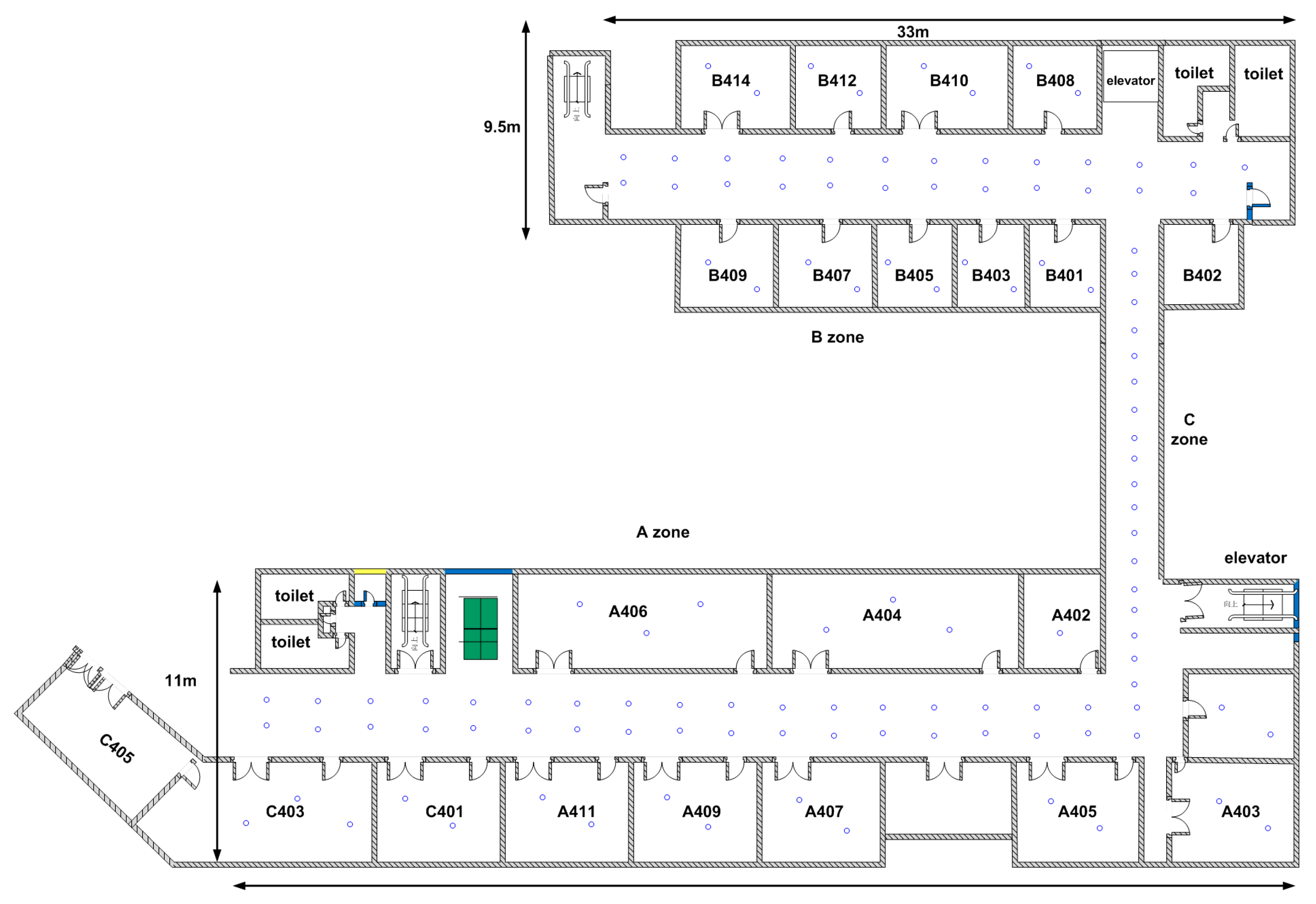
Our experimental field is the fourth floor of the building of Environmental Science and Spatial Informatics School at the China University of Mining and Technology (CUMT), the layout of which is depicted in Figure 2. This is a typical office environment including several offices, conference rooms and halls where nearly 30 APs are detected. We deploy reference locations in corridors and rooms. The blue circles in Figure 2 represent reference locations. We deploy a reference location every three meters along the middle line in the narrow corridor of c-zone, whereas in other wide corridors, we divide the interest areas into grids of 2.5 m by 2.5 m and deploy reference locations on the four corners of the grids. Depending on the size of the room, each room is evenly deployed with two to three reference locations. Overall, the whole field has an area of about 800 square meters, which is modeled as a space of about 120 reference locations.
We collect two types of samples: labeled samples and unlabeled samples. We select four volunteers who carry different mobile devices to collect labeled RSS samples at each reference location one at a time. By using our self-developed collecting program installed on the mobile device, each person collects 20 samples at each reference location at the frequency of 2 Hz and meanwhile inputs the location coordinates through the user interface. The four different mobile devices involved are an ASUS laptop, a MI smartphone, a Huawei smartphone, and a Huawei pad. The collecting program contains two versions that are implemented on Android and Windows systems. Finally, we have 80 labeled samples at each reference location, for a total of 9600 labeled samples throughout the whole experimental field. The proposed Co-Forest only use a small number of labeled samples as well as some unlabeled samples. To obtain unlabeled samples, we pick one volunteer from each office in the experimental field, so that the distribution of unlabeled samples would cover the entire experimental field. As mentioned above, volunteers complete their daily work in their offices, while the acquisition program running in the background of their mobile devices collects unlabeled RSS samples from surrounding APs and uploads them to the fingerprint server. This implicit collection process does not require users’ active interaction, and is running without the user being aware. The start and end of the acquisition work is controlled by a message sent by the server. These unlabeled samples are exploited by Co-Forest to augment the ensemble classifier. In addition, to analyze the feature of the RSS samples from the heterogeneous devices and verify the preprocessing method, we specially collect a set of samples contributed by diverse devices at a few fixed reference locations, which are used in Section 4.2.
4.2. Experimental Analysis on the Difference in RSS Samples of Heterogeneous Devices and Comparison between Processed and Raw Samples
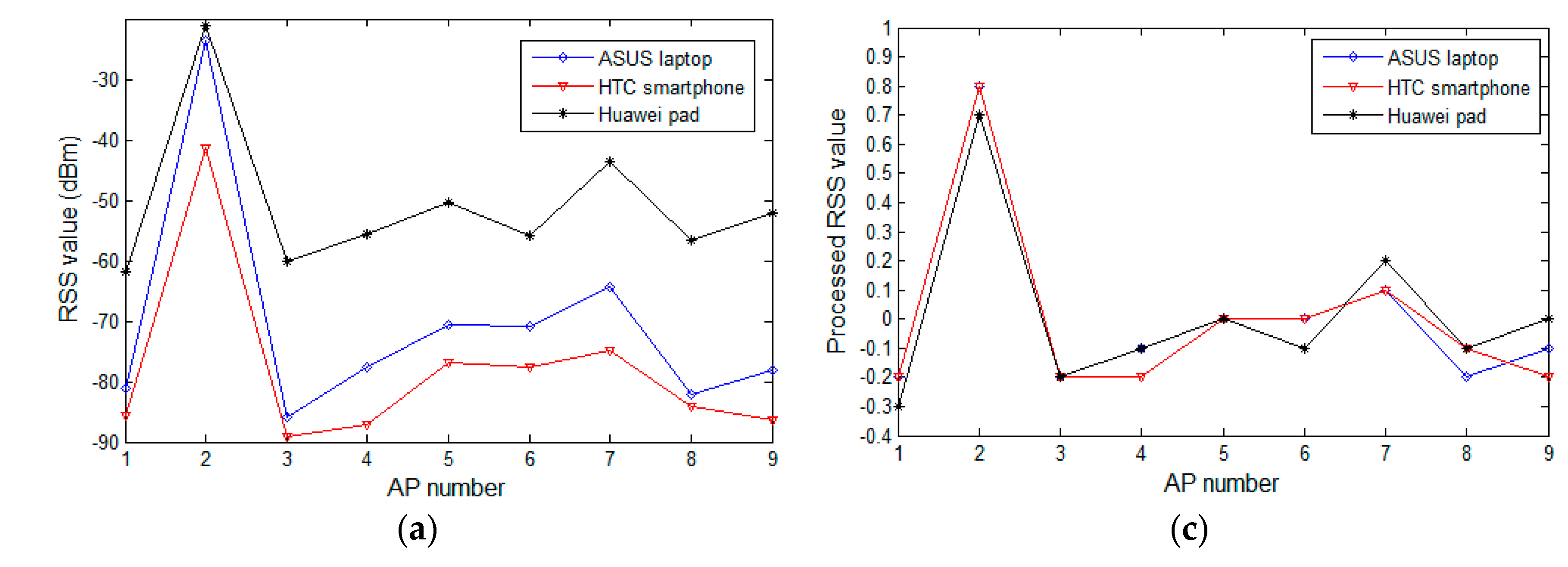
In this section, we review the experimental analysis on the difference in RSS values from heterogeneous devices and verify the effectiveness of the proposed preprocessing method. At a few selected reference locations in the experimental field, we use heterogeneous mobile devices to collect RSS samples from the surrounding APs that are subsequently processed by the proposed preprocessing method. The fluctuation curves of the raw and processed samples are depicted and compared in Figure 3. Figure 3a,b displays the raw RSS values of the surrounding AP change versus AP numbers at reference locations three and five, respectively. Figure 3c corresponds to the processing result of Figure 3a, while Figure 3d corresponds to the processing result of Figure 3b. In Figure 3a,b, the observing devices are heterogeneous, and are different in terms of software or hardware. The mobile devices used in Figure 3a are the ASUS A540 laptop (ASUS, Taipei, Taiwan) running WINDOWS 10 (Microsoft, Redmond, WA, USA), the HTC Desire 830 (HTC, Hsinchu, Taiwan) powered by Android 5.1 (Google, Mountain city, Santa Clara, CA, USA), and the Huawei M2 (Huawei, Shenzhen, China) powered by Android 5.1. In Figure 3b, the devices are a Lenovo Z501laptop (Lenovo, Beijing, China) running WINDOWS 7 (Microsoft, Redmond, WA, USA), a Huawei Honor 7 (Huawei, Shenzhen, China) powered by Android 6.0 (Google, Mountain city, Santa Clara, CA, USA), and a MI note (Xiaomi, Beijing, China) powered by Android 5.0 (Google, Mountain city, Santa Clara, CA, USA). Even for the same AP, the raw RSS observed by heterogeneous devices are obviously different. Specifically, in Figure 3a, the average RSS difference for all the APs between the Huawei pad and ASUS laptop is about 20 dBm, where the smallest gap is about 2.7 dBm on AP2, and on AP9 the maximum difference is up to 26 dBm. Although the curves of the HTC smartphone and the ASUS laptop are relatively close, an average RSS difference of 7.6 dBm exists between them. In Figure 3b, a similar situation at the reference location five is also seen.
Although the RSS values differ between heterogeneous devices, the RSS curves of all the devices display a relatively consistent fluctuating trend. At a particular reference location, these RSS samples collected by different devices seem to have some essential information in common: the RSS value sorting order of all the detectable APs. This is because the RSS collected from a nearby AP is higher than that from a distant AP for a particular mobile device. This rule does not change with the choice of observing device. The goal of our preprocessing method is to map all the RSS values to a uniform range to overcome the influence of the differences in RSS on the positioning system, under the premise of preserving the essential information of the crowdsourcing RSS samples. In Figure 3c,d, the curves of the processed data are fairly close, and even coincident for some APs. The effects of the heterogeneous devices are significantly reduced, while the curves of the preprocessed data maintain the same trend as the raw data curves, indicating that the essential information in the raw crowdsourcing samples is preserved.
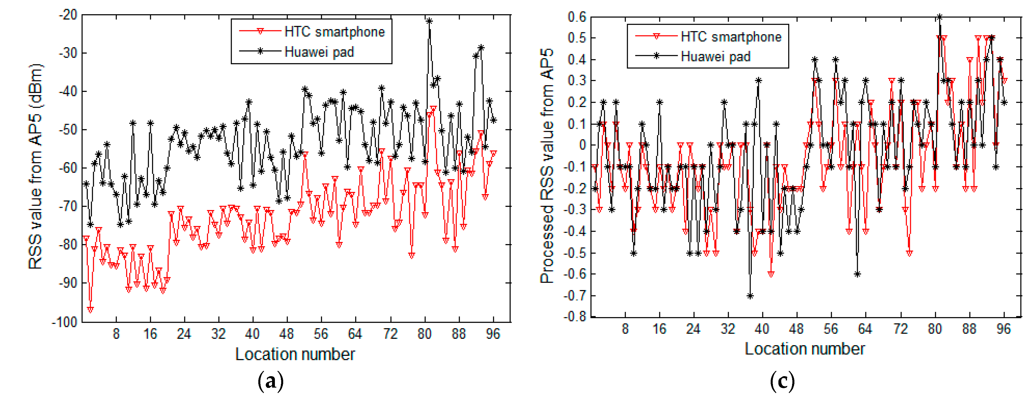
From another point of view, we fix APs and study the change in RSS values collected by heterogeneous devices at different observation locations. Figure 4a,b depicts the curves of raw RSS values of fixed access points AP5 and AP11, respectively, which are collected at 96 reference locations. Figure 4c corresponds to the processing result of Figure 4a, while Figure 4d corresponds to the processing result of Figure 4b. The two heterogeneous devices are a HTC smartphone and a Huawei pad. Similarly, in Figure 4a,b, the raw RSS values of selected APs, collected by heterogeneous devices, differ significantly at each reference location. In Figure 4c,d, the curves of the processed data are essentially coincident, showing the preprocessing method’s ability of managing differences in the signal strength of heterogeneous devices. To test the preprocessing method, we plot and compare curves of raw data and processed data that are collected from a large number of APs at a wide range of reference locations. However, due to space limitations, we have only provided some typical experimental results. In Figure 3, we display the data of reference locations three and five, while, in Figure 4, we show the data from AP5 and AP11.
The preprocessing method also realizes the discretization of continuous RSS values in the crowdsourcing samples, which greatly reduces the number of distinct RSS values on each AP in the samples, and hence helps improve the speed of constructing the random forest in the subsequent process. Figure 5 shows the comparison of the number of distinct RSS values on each AP between the raw samples and the processed samples. After preprocessing, the average number of distinct RSS values on APs decreases by 76%, from 73 to 17.
Each time the tree construction algorithm tries to determine the best attribute to select, the information theoretic index of each attribute has to be calculated. For a continuous attribute containing N values, the algorithm needs N − 1 times calculations and each calculation corresponds one kind of splitting on this attribute. The index is the optimal value of the N − 1 results. However, for discrete attributes, the algorithm only needs a one-time calculation to obtain the index. Therefore, continuous attributes increase the time and space consumption of the tree-constructing algorithm. From the data in Figure 5, the amount of computation savings for each APs is shown in Table 3, with a maximum of a 78% savings for AP2 and a minimum of 63% for AP5. Therefore, replacing continuous values in each AP with discrete values can greatly reduce the amount of computation required, improving the efficiency of constructing decision trees and even the training speed of the whole random forest.
4.3. Effect of Preprocessing Method on Tackling Device Heterogeneity
We study the effect of the proposed min–max preprocessing method for addressing the RSS sample variation of the different devices. To depict the crowdsourcing sampling, the samples observed by the different devices are used. The test is conducted on 90 randomly selected reference locations. For each reference location, the 60 labeled RSS samples collected by the ASUS laptop, MI smartphone, and Huawei pad are used as training samples, whereas the 20 samples collected by the Huawei smartphone are used as the test samples. Therefore, 5400 training samples and 1800 test samples are used. First, we apply the proposed min–max method, as well as other existing preprocessing methods, including DIFF and SSD, to manage the training and test sample set. Subsequently, the location estimation algorithms that are trained by the training sample set make a prediction for the test sample. For comparison, the RSS method is added, which only use the raw RSS sample set without preprocessing. To estimate location, we select three typical algorithms: k Nearest Neighbors (k-NN), Naive Bayes (NB), and Classification and Regression Trees (CART). The effects of the preprocessing methods are evaluated by comparing the positioning accuracy of the strategies that fuse various preprocessing methods and estimation algorithms. The positioning accuracy is measured as the cumulative distribution function (CDF) of error distances that are calculated as the Euclidean distances between the prediction coordinates results and the actual coordinates. The CDF plots for k-NN, NB and CART are shown in Figure 6a–c, respectively.
Min–max outperforms the other typical preprocessing methods regardless of the estimation algorithm used. Compared to RSS, the probability of error distance within five meters for min–max is better by 12%, 21%, and 13%, as shown in Figure 6a–c, respectively. Other preprocessing algorithms also improve the overall accuracy, while the RSS method has the worst performance. This illustrates the adverse influence of heterogeneous device signal variation on positioning accuracy and the importance of using preprocessing methods. In Figure 6a,b, the min–max method behaves slightly better than DIFF. To achieve this performance, DIFF needs additional storage space. In terms of our training sample set (5400 samples, 25 APs per sample), the DIFF method has to store 1,485,000 more signal values in the fingerprint database than the min–max method. In addition, the SSD method has poorer performance than the DIFF method, even though they are based on the same idea of using the difference in signal values. To reduce the storage requirement, the SSD method only preserves the difference between adjacent APs, and some useful information is abandoned, which may affect the performance. In Figure 6c, the min–max method exhibits a significant improvement compared to the other methods. Given the good performance of min–max in handling the sample set for the decision tree model, we choose min–max as the preprocessing method for the sample set used by our proposed Co-Forest algorithm.
Notably, the choice of parameter k of k-NN is dependent on the dataset used. However, this is not the focus of our study, we only provide the final selected value after tuning operations, k = 4. We find that the probabilistic algorithm NB perform worse than the other estimation algorithms, especially when the raw samples without preprocessing are used. This seems to be inconsistent with the existing findings that probabilistic algorithms usually perform better than deterministic algorithms. The possible explanation for this is that NB will have good accuracy when enough samples are available to describe the probability distribution of the features. However, from each device, we only obtain 20 training samples at each reference location. The insufficient number of samples and the effect of signal variation reduce the accuracy of NB.
4.4. Selection of the Number of Trees in the Random Forest
An important parameter of Co-Forest is N, the number of trees in the random forest. The model performance can improve with increasing N, when N is small. However, as previously indicated [33], when N reaches a certain value, the overhead of the algorithm increases as the value of N increases, but the performance of the model does not increase accordingly. We use the out-of-bag (OOB) error to measure the random forest performance and attempt to determine the optimal value of N by observing the change in the OOB error value with the increase in N. OOB error has been shown to be the unbiased error estimate of the random forest, which can be obtained without cross validation [34]. To illustrate the OOB error definition, we first define the OOB data and the set of OOB decision trees. Assuming the labeled samples set is L and the bootstrap samples set is denoted as , which is the bootstrap sampled from L in order to generate component decision tree of the forest. Then, for each sample (, L, the probability of not being selected is , where m is the count of samples in L. When the value of m is large enough, . In other words, about 36.8% of the samples in L are not in . These data are called out-of-bag (OOB) data, which can be used to validate the model because they are not used to train the model. Conversely, for each of L, there are several that do not contain ; moreover, a set of decision trees can be generated using these , which are called OOB trees of . Now, the definition of OOB error is given as:
where indicates the prediction result of by its OOB trees, which is the combination of prediction results of each tree through majority voting. The function is the indicator function. The function value is 1 when the prediction result is equal to , otherwise the value is 0. Namely, the OOB error is the mean prediction error on each training sample , using only trees generated by bootstrap sample sets that do not contain .
To obtain the optimal value of N, in our labeled samples set and the processed data set, we constantly adjust the values of N and calculate the OOB error value of the generated random forests. Figure 7 shows how the OOB error values change with the number of random trees. From both of the curves, when N is small (less than 20), the OOB error decreases rapidly as N increases. When N is greater than 30, the OOB error no longer changes significantly as N increases. Therefore, for our experimental dataset, we select 30 as the optimal value of N. In addition, we find that the OOB error of the processed dataset is reduced by 6% on average compared with the raw dataset because the preprocessing method reduces the influence of crowdsourcing RSS sample variance on the prediction accuracy.
4.5. Positioning Accuracy Comparison of Co-Forest and Classical Algorithms
To evaluate the performance of the proposed Co-Forest algorithm, we first compare the positioning accuracy of Co-Forest with several existing positioning algorithms, including the k-NN algorithm and two other semi-supervised learning algorithms, SSLLE and FCO-SVR. As one of the classic indoor positioning methods, k-NN is always used for comparison by researchers. It is a supervised learning method that only uses labeled samples. As mentioned above, the selection of k is data-dependent and we use the selected value of four for k, with which we almost obtain the best accuracy of k-NN in this dataset. As introduced in Section 2, the SSLLE method first uses the dimension reduction technique of locally linear embedding (LLE) to map high dimensional RSS vectors into a low dimensional space and then applies a semi-supervised multiclass label propagation algorithm to train the fingerprint database. We implement the method and set the number of nearest neighbors to k = 5 as Jain et al. do [19]. The FCO-SVR method employs the unlabeled samples to train and update a pair of support vector regression (SVR) learners, which is similar to our algorithm. However, only two learners are used and refined in the traditional co-training method. To improve the system performance, we extend the number of component classifiers to multiple and adopt a more efficient method to obtain the most confidential samples. Here, the number of trees in Co-Forest is 30.
All of the three semi-supervised methods use both labeled and unlabeled samples. Therefore, we extract both the labeled and unlabeled samples for training from the experimental sample set. The labeled sample set contains a total of 6400 samples and 80 reference locations. At each reference location, 80 labeled samples are collected. The unlabeled sample set contains 3200 unlabeled samples that are secretly collected by crowdsourcing volunteers. In addition, 60 reference points are selected as test locations, and 10 samples are collected at each reference point, for 600 test samples. To address the variation in RSS samples due to the differences in devices, all the samples in training and test sets are processed in advance by the min–max preprocessing method. For ease of comparison, other than the 3200 unlabeled samples, the three semi-supervised algorithms only use half of the labeled sample sets, i.e., 3200 labeled samples from 80 reference locations with 40 samples per reference location. However, the k-NN algorithm runs on both the half-labeled sample set and the entire set of labeled samples. The CDF plots of error distances for these algorithms are shown in Figure 8, and the comparison of the mean error, maximum error, minimum error, and median error for these algorithms are shown in Table 4.
We find that the performance of the k-NN algorithm is much better when the number of labeled training samples increase from 3200 to 6400. This may reflect the dependency of a supervised learning algorithm, such as k-NN, on the number of labeled training samples. With the help of unlabeled samples, the several semi-supervised algorithms using only half of the labeled samples obtain comparable, or better, positioning performance than k-NN which uses the entire labeled sample set. This demonstrates that semi-supervised learning techniques can help reduce the number of labeled samples used in indoor positioning by exploiting the value of many unlabeled samples. In particular, Co-Forest outperforms the other two semi-supervised algorithms. The probability of error distance within three meters for Co-Forest is better by 10% and 8% compared to FCO-SVR and SSLLE, respectively. The mean error distance is reduced by 12% and 18%, respectively. In addition, the maximum error distance of SSLLE is much higher than Co-Forest and FCO-SVR, and its probability of error distance beyond five meters is significantly decreased. This reflects the instability of SSLLE, which may be affected by the selection of the parameter k. The result from SSLLE is sensitive to the value of the parameter k, i.e., the number of nearest neighbors used in the algorithm.
We also evaluate the algorithm’s performance under adverse conditions. When there are multiple persons moving around in an indoor environment, the Wi-Fi signals will be blocked and the observation of RSS samples will become unstable or even incomplete, which decreases the algorithm performance. On the five working days a few pedestrians are in the corridors, we collect the test samples to estimate locations and compare the mean error distances of these algorithms. A total of 500 test samples are collected, and the test locations almost cover all of the corridors in the experimental field. The performance of the algorithms under adverse conditions is shown in Table 5. Compared with the mean error distances in Table 4, the performance of these algorithms all decreases. However, k-NN and SSLLE are affected more adversely, and the mean error distances increase by 87% and 93%, respectively. The mean error distances for Co-Forest and FCO-SVR also increase 51% and 64%, respectively. However, the error distance of Co-Forest is within four meters in this situation, which is acceptable.
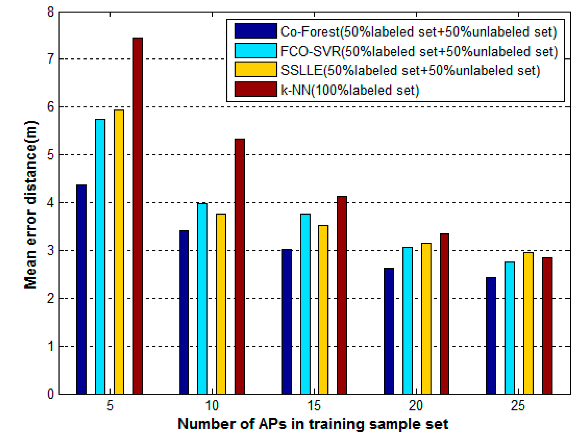
The WLAN indoor positioning algorithm results are easily affected by changes in the WLAN environment, such as the addition or removal of APs. We try to evaluate the robustness of these algorithms by comparing their performance when we adopt different numbers of APs in the training sample set. The training sample set we used above contains, at most, 30 detectable APs, 25 of which have enough values for positioning. Therefore, we set the number of APs in the training sample set to 5, 10, 15, 20, and 25, and record the mean error distances of these algorithms in each case. For simplicity, k-NN is only tested on the entire training dataset containing 6400 labeled samples. The mean error distances versus the number of APs in the training sample set for these algorithms are shown in Figure 9. The mean error distances of these algorithms all increase as the numbers of APs decrease. When the number of APs drops to five, all the algorithms perform poorly, and the mean error of k-NN even increase to 7.44 m. In addition, the change trends of each algorithm vary. In the most extreme case, when the number of APs drops from 25 to 5, the mean error distance of k-NN grows from 2.84 m to 7.44 m, improving by 161%. In the same case, the Co-Forest results increase from 2.42 m to 5 m, an improvement of 80%. Overall, the average change distances for Co-Forest, FCO-SVR, SSLLE, and k-NN are 0.59 m, 0.90 m, 0.93 m, and 1.37 m, respectively. Therefore, as the number of APs varies, the Co-Forest results change more gradually than the others, which indicates the robustness of the proposed algorithm.
5. Conclusions and Future Work
In this paper, we propose a novel WLAN fingerprint positioning strategy, which combines implicit crowdsourcing sampling with a semi-supervised learning algorithm to effectively bypass the traditional labor-intensive task of fingerprint collection. The implicit crowdsourcing sampling technique is able to collect unlabeled RSS samples faster since it does not require user interaction like the classical crowdsourcing technique. The proposed preprocessing method completes the normalization and discretization of the crowdsourcing RSS samples that are contributed by a range of heterogeneous devices, and succeeds in addressing the challenge of the variance in RSS samples from heterogeneous devices in crowdsourcing sampling and assists in the quick training of the ensemble classifier. Combining ensemble learning with a collaborative training paradigm, the new semi-supervised learning method, Co-Forest, uses a large number of unlabeled samples to generate and refine a random forest classifier that achieves comparable positioning performance compared to classical algorithms that use more labeled samples.
In the future, more experiments in real indoor environments will be conducted and the system practicality will be further investigated. Additionally, improving the system accuracy when the number of samples is relatively small at the beginning of crowdsourcing sampling is another research aspect.
Acknowledgments
This work is supported by the National Key Research and Development Program of China (2016YFC0803103).
Author Contributions
Chunjing Song proposed the research and drafted the manuscript. Jian Wang was involved in the writing of the manuscript and in responding to the reviewers’ comments.
Conflicts of Interest
The authors declare no conflict of interest.
References
- Hightower, J.; Borriello, G. A survey and taxonomy of location systems for ubiquitous computing. IEEE Comput. 2001, 34, 57–66. [Google Scholar] [CrossRef]
- Liu, H.; Darabi, H.; Banerjee, P.; Liu, J. Survey of wireless indoor positioning techniques and systems. IEEE Trans. Syst. Man Cybern. C 2007, 37, 1067–1080. [Google Scholar] [CrossRef]
- He, S.N.; Chan, S.H.G. Wi-Fi fingerprint-based indoor positioning: Recent advances and comparisons. IEEE Commun. Surv. Tutor. 2016, 18, 466–490. [Google Scholar] [CrossRef]
- Li, X.; Wang, J.; Liu, C.; Zhang, L.; Li, Z. Integrated WiFi/PDR/smartphone using an adaptive system noise extended Kalman filter algorithm for indoor localization. ISPRS Int. J. Geo-Inf. 2016, 5, 8. [Google Scholar] [CrossRef]
- Xia, S.X.; Liu, Y.; Yuan, G.; Zhu, M.; Wang, Z. Indoor Fingerprint Positioning based on Wi-Fi: An Overview. ISPRS Int. J. Geo-Inf. 2017, 6, 135. [Google Scholar] [CrossRef]
- Hossain, A.K.M.; Soh, W.-S. A survey of calibration-free indoor positioning systems. Comput. Commun. 2015, 66, 1–13. [Google Scholar] [CrossRef]
- Dong, F.; Chen, Y.; Liu, J.; Ning, Q.; Piao, S. A calibration-free localization solution for handling signal strength variance. In Proceedings of the International Conference on Mobile Entity Localization and Tracking in Gps-Less Environments, Orlando, FL, USA, 30 September 2009; pp. 79–90. [Google Scholar]
- Bolliger, P. Redpin-adaptive, zero-configuration indoor localization through user collaboration. In Proceedings of the ACM International Workshop on Mobile Entity Localization and Tracking in Gps-Less Environments, San Francisco, CA, USA, 19 September 2008; pp. 55–60. [Google Scholar]
- Luo, Y.; Hoeber, O.; Chen, Y. Enhancing Wi-Fi fingerprinting for indoor positioning using human-centric collaborative feedback. Hum.-Cen. Comput. Inf. Sci. 2013, 3, 2. [Google Scholar] [CrossRef] [Green Version]
- Hossain, A.K.M.; Van, H.N.; Soh, W.-S. Utilization of user feedback in indoor positioning system. Perv. Mob. Comput. 2010, 6, 467–481. [Google Scholar] [CrossRef]
- Ledlie, J.; Park, J.G.; Curtis, D.; Cavalcante, A. Mole: A scalable, user-generated WiFi positioning engine. In Proceedings of the International Conference on Indoor Positioning and Indoor Navigation, Guimaraes, Portugal, 21–23 September 2011; pp. 1–10. [Google Scholar]
- Park, J.G.; Charrow, B.; Curtis, D.; Battat, J.; Minkov, E.; Hicks, J. Growing an organic indoor location system. In Proceedings of the International Conference on Mobile Systems, Applications, and Services, San Francisco, CA, USA, 15–18 June 2010; pp. 271–284. [Google Scholar]
- Hossain, A.K.M.; Jin, Y.; Soh, W.-S.; Van, H.N. SSD: A robust rf location fingerprint addressing mobile devices’ heterogeneity. IEEE Trans. Mob. Comput. 2013, 12, 65–77. [Google Scholar] [CrossRef]
- Kim, W.; Yang, S.; Gerla, M.; Lee, E.K. Crowdsource based Indoor Localization by Uncalibrated Heterogeneous Wi-Fi devices. Mob. Inf. Syst. 2016, 2016, 1–18. [Google Scholar] [CrossRef]
- Machaj, J.; Brida, P.; Piché, R. Rank based fingerprinting algorithm for indoor positioning. In Proceedings of the International Conference on Indoor Positioning and Indoor Navigation, Guimaraes, Portugal, 21–23 September 2011; pp. 1–6. [Google Scholar]
- Rai, A.; Chintalapudi, K.K.; Padmanabhan, V.N.; Sen, R. Zee: Zero-effort crowdsourcing for indoor localization. In Proceedings of the MobiCom’12, Istanbul, Turkey, 22–26 August 2012; pp. 293–304. [Google Scholar]
- Wu, C.; Yang, Z.; Liu, Y.; Xi, W. WILL: Wireless indoor localization without site survey. IEEE Trans. Parallel Distrib. Syst. 2013, 24, 839–848. [Google Scholar]
- Wang, H.; Sen, S.; Mariakakis, A.; Youssef, M. Demo: Unsupervised indoor localization. In Proceedings of the International Conference on Mobile Systems, Applications, and Services, Lake District, UK, 26–29 June 2012; pp. 499–500. [Google Scholar]
- Jain, V.K.; Tapaswi, S.; Shukla, A. Location estimation based on semi-supervised locally linear embedding (sslle) approach for indoor wireless networks. Wirel. Pers. Commun. 2012, 67, 879–893. [Google Scholar] [CrossRef]
- Xia, Y.; Ma, L.; Zhang, Z.Z.; Zhou, C.F. Wlan Indoor Positioning Algorithm based on Semi-supervised Manifold Learning. J. Syst. Eng. Electron. 2014, 36, 1423–1427. [Google Scholar]
- Zhang, Y.; Zhi, X.L. Indoor Positioning Algorithm Based on Semi-supervised Learning. Comput. Eng. 2010, 36, 277–279. [Google Scholar]
- Xia, M. Semi-Supervised Learing Based Indoor WLAN Positioning. Ph.D. Thesis, Chongqing University of Posts and Telecommunications, Chongqing, China, 2016. [Google Scholar]
- Goswami, A.; Ortiz, L.E.; Das, S.R. Wigem: A learning-based approach for indoor localization. In Proceedings of the 7th International Conference on Emerging Networking Experiments and Technologies (CoNEXT), Tokyo, Japan, 6–9 December 2011; pp. 1–12. [Google Scholar]
- Laoudias, C.; Zeinalipour-Yazti, D.; Panayiotou, C.G. Crowdsourced indoor localization for diverse devices through radiomap fusion. In Proceedings of the International Conference on Indoor Positioning and Indoor Navigation, Montbeliard-Belfort, France, 28–31 October 2013; pp. 1–7. [Google Scholar]
- Cho, Y.; Ji, M.; Lee, Y.; Park, S. WiFi AP position estimation using contribution from heterogeneous mobile devices. In Proceedings of the IEEE/ION Position Location and Navigation Symposium (PLANS), Myrtle Beach, SC, USA, 24–26 April 2012; pp. 562–567. [Google Scholar] [CrossRef]
- Jain, Y.K.; Bhandare, S.K. Min Max Normalization Based Data Perturbation Method for Privacy Protection. Int. J. Comput. Commun. Technol. 2011, 2, 45–50. [Google Scholar]
- Gajera, V.; Shubham; Gupta, R.; Jana, P.K. An effective Multi-Objective task scheduling algorithm using Min-Max normalization in cloud computing. In Proceedings of the International Conference on Applied and Theoretical Computing and Communication Technology, Bengaluru, India, 21–23 July 2016; pp. 812–816. [Google Scholar]
- Song, C.J.; Wang, J.; Yuan, G. Hidden naive bayes indoor fingerprinting localization based on best-discriminating ap selection. ISPRS Int. J. Geo-Inf. 2016, 5, 189. [Google Scholar] [CrossRef]
- Li, M.; Zhou, Z.H. Improve Computer-Aided Diagnosis with Machine Learning Techniques Using Undiagnosed Samples. IEEE Trans. Syst. Man Cybern. Part A Syst. Hum. 2007, 37, 1088–1098. [Google Scholar] [CrossRef]
- Blum, A.; Mitchell, T. Combining labeled and unlabeled data with co-training. In Proceedings of the Eleventh Conference on Computational Learning Theory, Madison, WI, USA, 24–26 July 1998; pp. 92–100. [Google Scholar]
- Jedari, E.; Wu, Z.; Rashidzadeh, R.; Saif, M. Wi-Fi based indoor location positioning employing random forest classifier. In Proceedings of the International Conference on Indoor Positioning and Indoor Navigation, Banff, AB, Canada, 13–16 October 2015; pp. 1–5. [Google Scholar]
- Górak, R.; Luckner, M. Modified Random Forest Algorithm for Wi–Fi Indoor Localization System. In Proceedings of the First International Conference on Computer Communication and the Internet, Wuhan, China, 13–15 October 2016; pp. 147–157. [Google Scholar]
- Oshiro, T.M.; Perez, P.S.; Baranauskas, J.A. How many trees in a random forest? Lect. Notes Comput. Sci. 2012, 7376, 154–168. [Google Scholar]
- Breiman, L. Random Forests. Mach. Learn. 2001, 45, 5–32. [Google Scholar] [CrossRef]
Figure 1.
Components of the proposed positioning system.
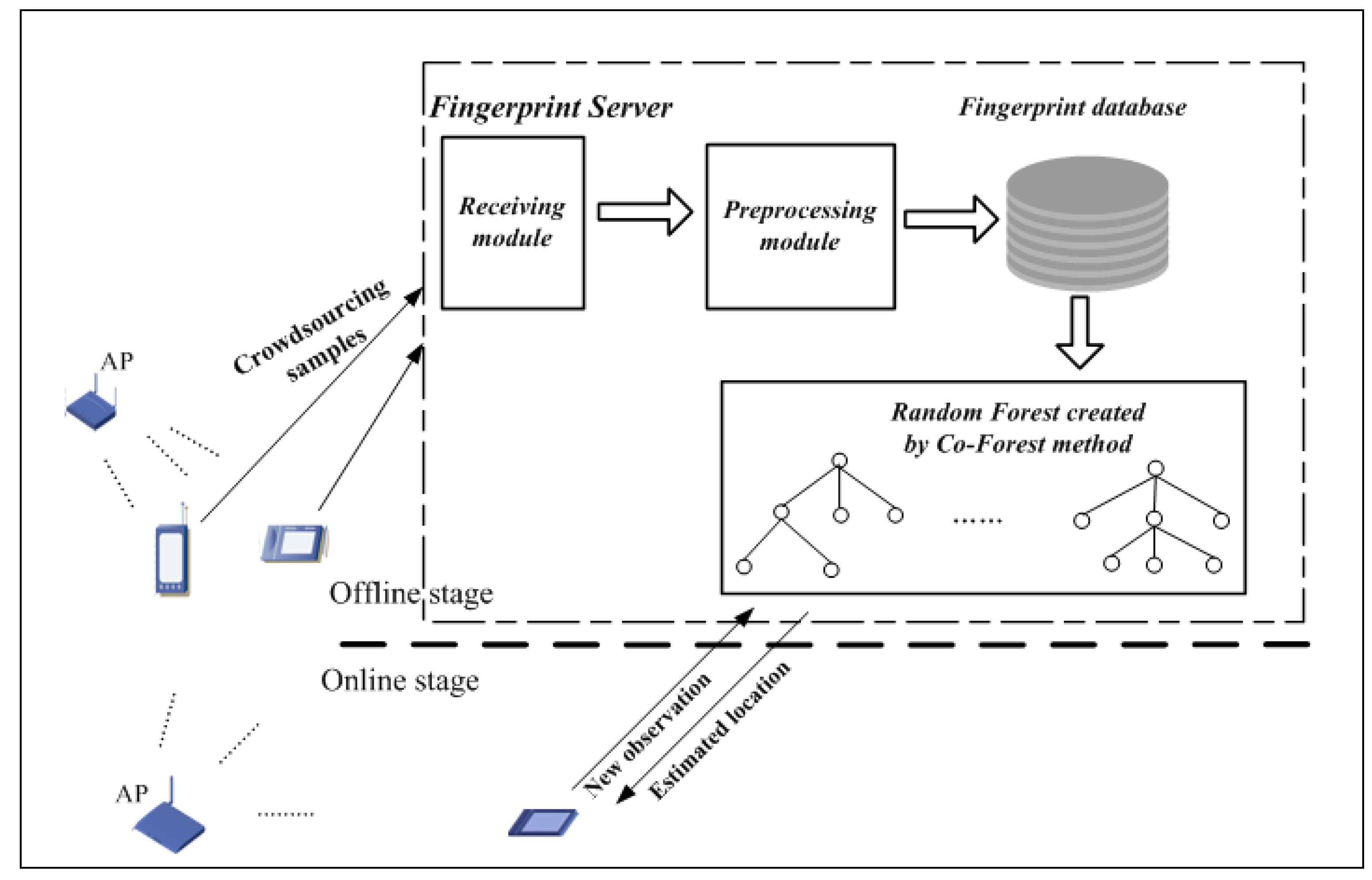
Figure 2.
Layout of the experimental field.

Figure 3.
RSS values change versus AP numbers: (a) the raw RSS values of the surrounding change in APs versus AP numbers at reference location three; (b) the raw RSS values of the change in surrounding APs versus AP numbers at reference location five; (c) the processing result of (a); and (d) the processing result of (b).

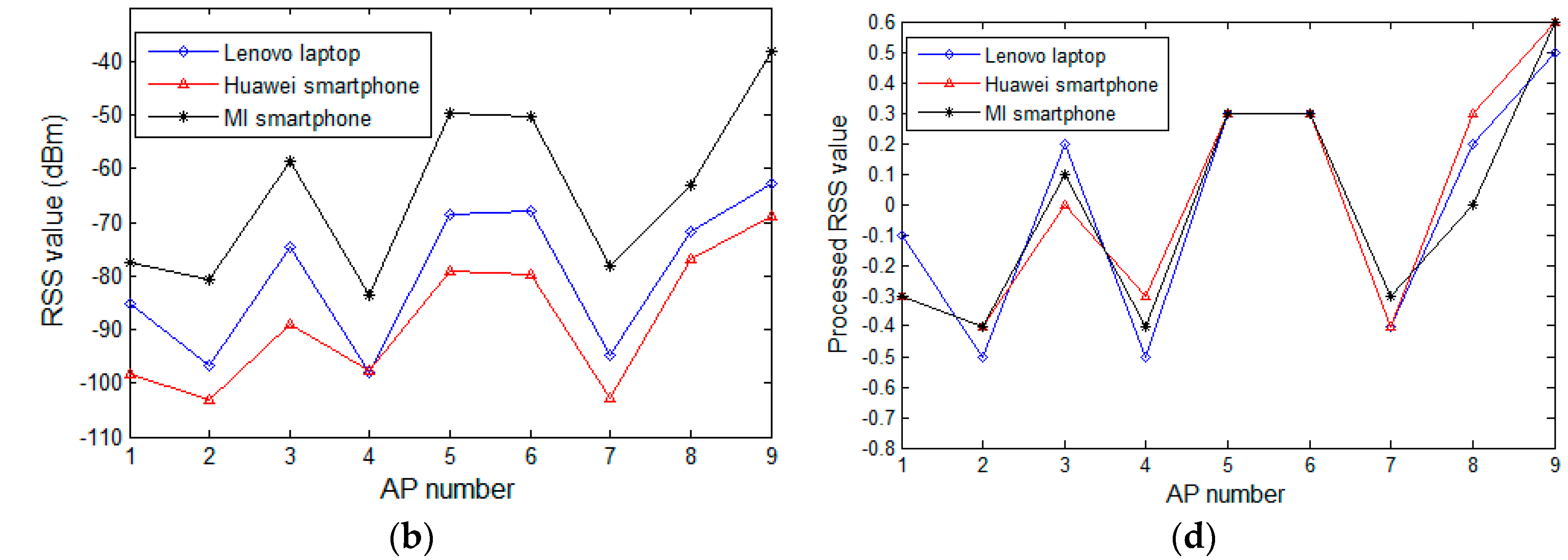
Figure 4.
RSS values change versus observation locations: (a) the change in raw RSS values of AP5 versus observation locations; (b) the change in raw RSS values of AP11 versus observation locations; (c) the processing result of (a); and (d) the processing result of (b).
Figure 4.
RSS values change versus observation locations: (a) the change in raw RSS values of AP5 versus observation locations; (b) the change in raw RSS values of AP11 versus observation locations; (c) the processing result of (a); and (d) the processing result of (b).

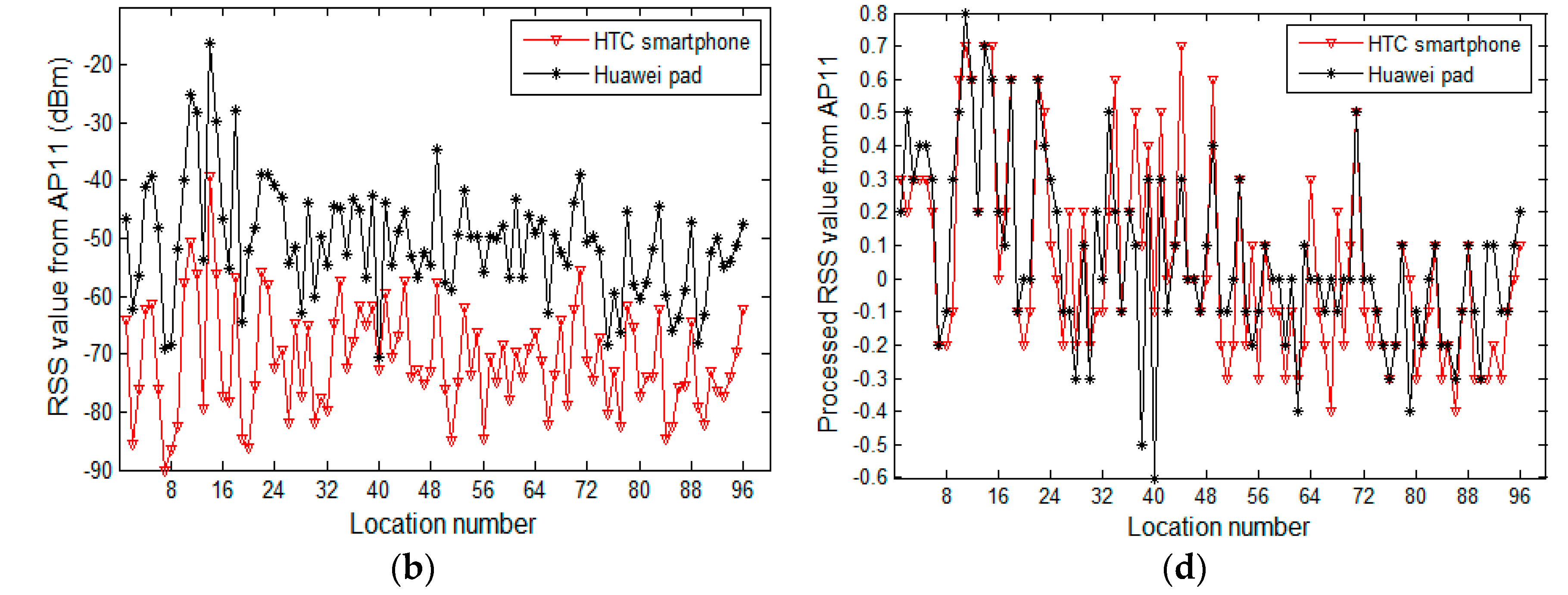
Figure 5.
Comparison of the number of distinct RSS values on each AP between the raw and processed samples.
Figure 5.
Comparison of the number of distinct RSS values on each AP between the raw and processed samples.
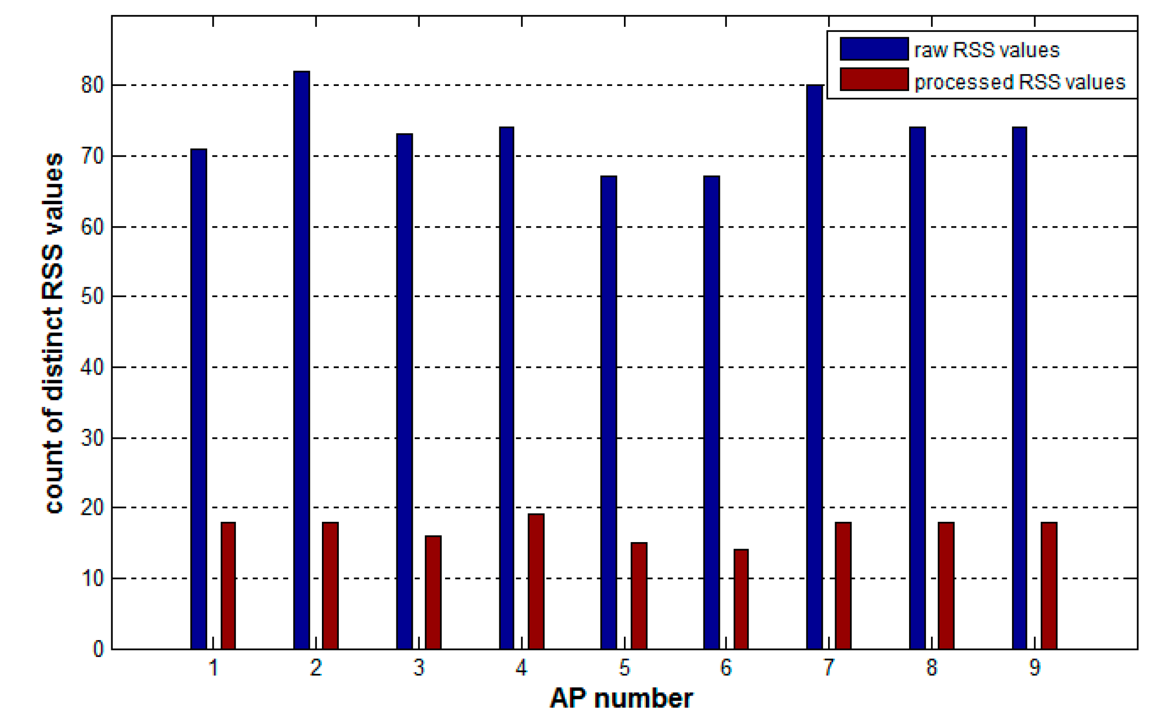
Figure 6.
Cumulative distribution function (CDF) plots of error distance for the different preprocessing methods: (a) k Nearest Neighbors (k-NN); (b) Naive Bayes (NB); and (c) Classification and Regression Trees (CART).
Figure 6.
Cumulative distribution function (CDF) plots of error distance for the different preprocessing methods: (a) k Nearest Neighbors (k-NN); (b) Naive Bayes (NB); and (c) Classification and Regression Trees (CART).
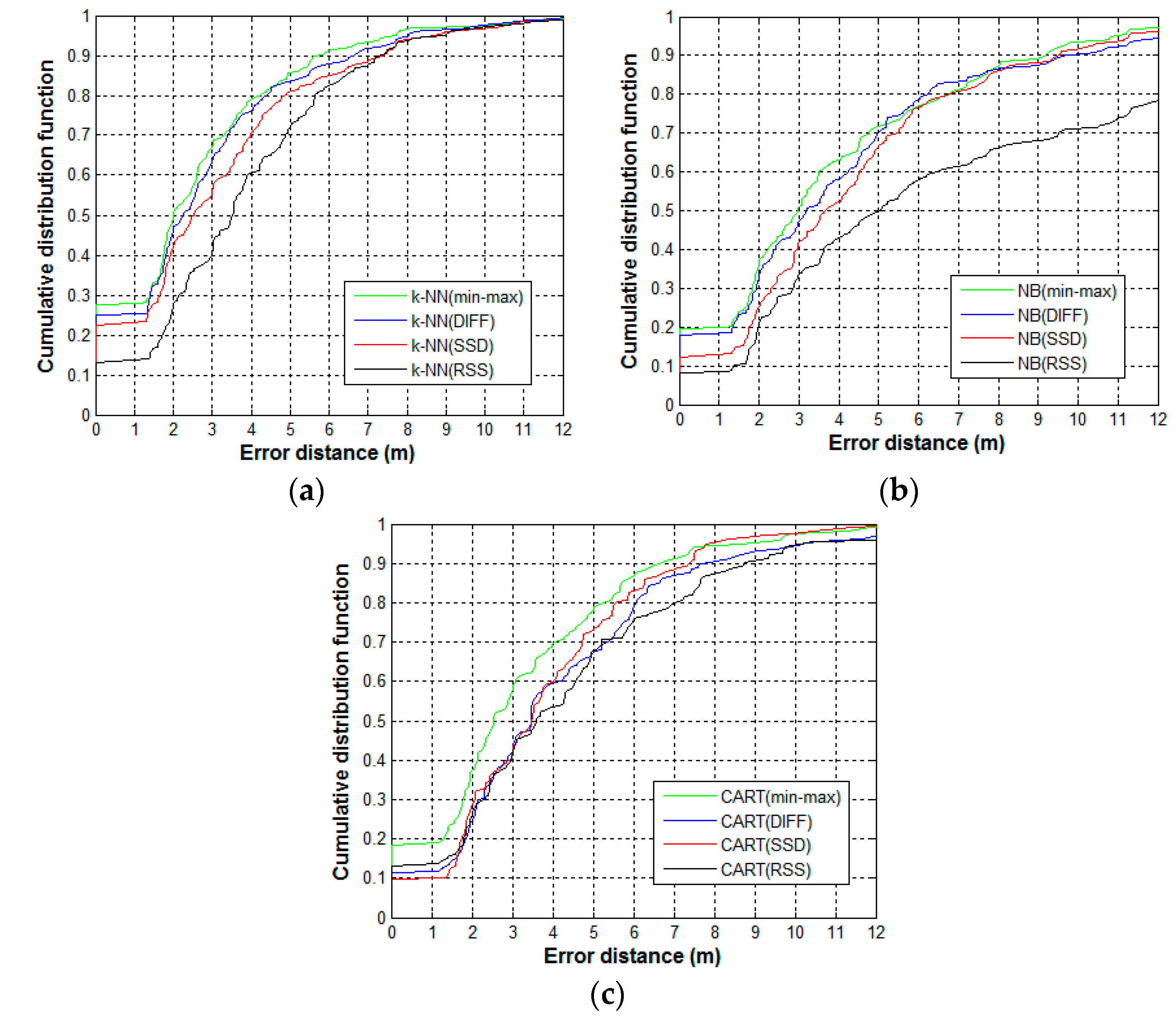
Figure 7.
Out-of-bag error of the processed and original labeled datasets.

Figure 8.
CDF plots of error distances for the four algorithms.
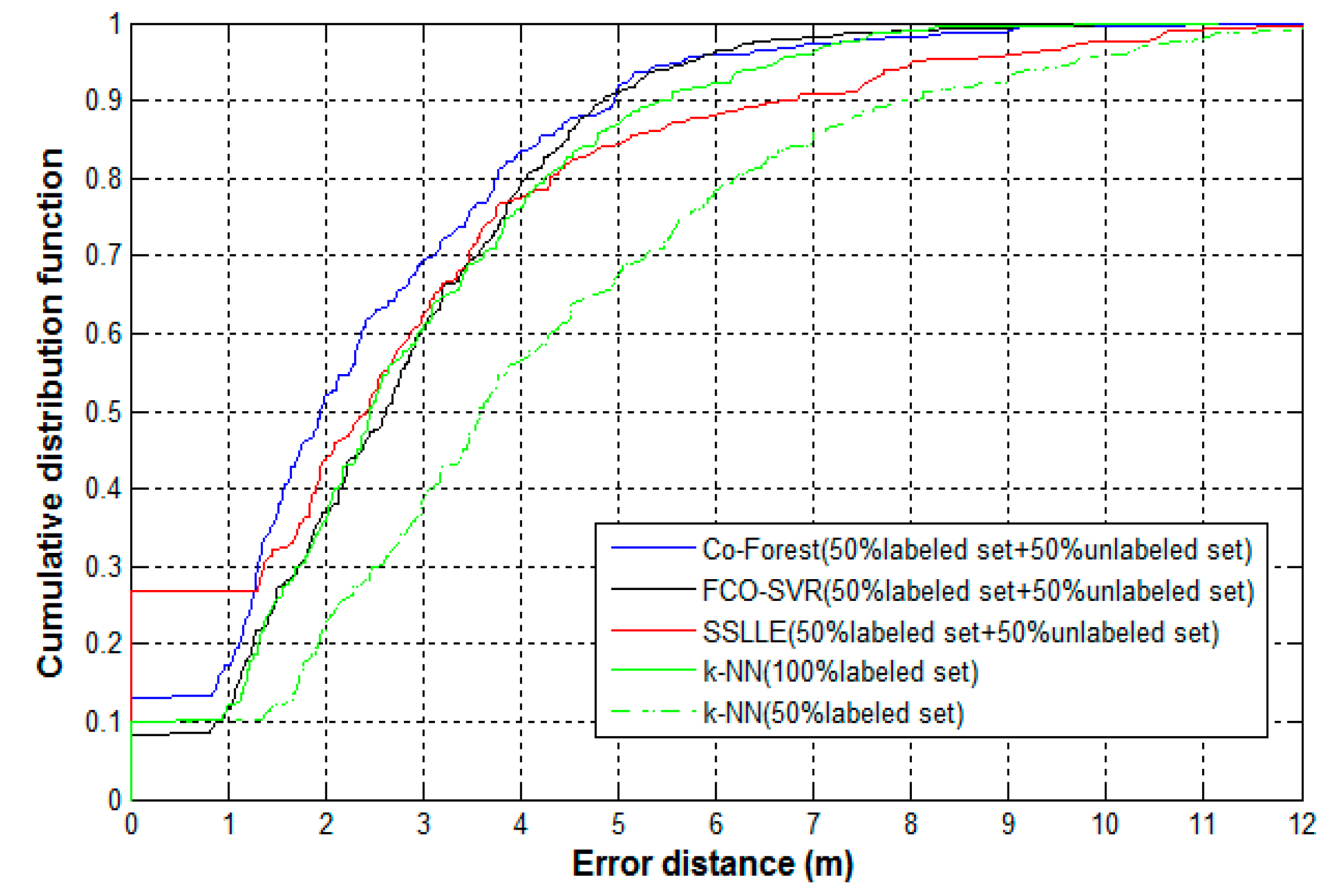
Figure 9.
The change in mean error distances of algorithms with the number of APs in the training sample set.
Figure 9.
The change in mean error distances of algorithms with the number of APs in the training sample set.

Table 1.
Raw crowdsourcing received signal strength (RSS) samples at a particular reference location.
Table 1.
Raw crowdsourcing received signal strength (RSS) samples at a particular reference location.
| Device | AP1 | AP2 | AP3 | AP4 | AP5 | AP6 |
|---|---|---|---|---|---|---|
| Device 1 | −85 | −42 | −89 | −77 | −76 | −89 |
| Device 2 | −81 | −35 | −76 | −70 | −77 | −85 |
| Device 3 | −83 | −40 | −85 | −84 | −72 | −90 |
| Device 4 | −67 | −18 | −64 | −61 | −53 | −67 |
| Device 5 | −79 | −35 | −87 | −72 | −73 | −81 |
Table 2.
Processed results of Table 1.
Table 2.
Processed results of Table 1.
| Device | AP1 | AP2 | AP3 | AP4 | AP5 | AP6 |
|---|---|---|---|---|---|---|
| Device 1 | −0.1 | 0.7 | −0.2 | 0.1 | 0.1 | −0.2 |
| Device 2 | −0.2 | 0.8 | −0.1 | 0.1 | −0.1 | −0.2 |
| Device 3 | −0.1 | 0.8 | −0.1 | −0.1 | 0.2 | −0.2 |
| Device 4 | −0.2 | 0.8 | −0.1 | −0.1 | 0.1 | −0.2 |
| Device 5 | −0.1 | 0.7 | −0.2 | 0.0 | 0.0 | −0.1 |
Table 3.
Reduction in the amount of computation for each access point (AP) from Figure 5.
Table 3.
Reduction in the amount of computation for each access point (AP) from Figure 5.
| AP1 | AP2 | AP3 | AP4 | AP5 | AP6 | AP7 | AP8 | AP9 | |
|---|---|---|---|---|---|---|---|---|---|
| Amount of Computation Saved | 64% | 78% | 69% | 67% | 63% | 64% | 75% | 68% | 68% |
Table 4.
Comparison of the mean error, maximum error, minimum error, and median error for the four algorithms.
Table 4.
Comparison of the mean error, maximum error, minimum error, and median error for the four algorithms.
| Algorithms | Mean Error (m) | Maximum Error (m) | Minimum Error (m) | Median Error (m) |
|---|---|---|---|---|
| k-NN (50% Labeled Set) | 4.05 | 11.95 | 0 | 3.59 |
| k-NN (100% Labeled Set) | 2.84 | 8.14 | 0 | 2.45 |
| SSLLE | 2.95 | 11.77 | 0 | 2.42 |
| FCO-SVR | 2.75 | 8.52 | 0.36 | 2.63 |
| Co-Forest | 2.42 | 8.03 | 0 | 1.95 |
Table 5.
The mean error distances of algorithms under adverse conditions.
| Algorithms | Mean Error (m) |
|---|---|
| k-NN (100% Labeled Set) | 5.31 |
| SSLLE | 5.69 |
| FCO-SVR | 4.51 |
| Co-Forest | 3.65 |
© 2017 by the authors. Licensee MDPI, Basel, Switzerland. This article is an open access article distributed under the terms and conditions of the Creative Commons Attribution (CC BY) license (http://creativecommons.org/licenses/by/4.0/).
Share and Cite
MDPI and ACS Style
Song, C.; Wang, J. WLAN Fingerprint Indoor Positioning Strategy Based on Implicit Crowdsourcing and Semi-Supervised Learning. ISPRS Int. J. Geo-Inf. 2017, 6, 356. https://doi.org/10.3390/ijgi6110356
AMA Style
Song C, Wang J. WLAN Fingerprint Indoor Positioning Strategy Based on Implicit Crowdsourcing and Semi-Supervised Learning. ISPRS International Journal of Geo-Information. 2017; 6(11):356. https://doi.org/10.3390/ijgi6110356
Chicago/Turabian StyleSong, Chunjing, and Jian Wang. 2017. "WLAN Fingerprint Indoor Positioning Strategy Based on Implicit Crowdsourcing and Semi-Supervised Learning" ISPRS International Journal of Geo-Information 6, no. 11: 356. https://doi.org/10.3390/ijgi6110356
Note that from the first issue of 2016, this journal uses article numbers instead of page numbers. See further details here.