A Dynamic Spatiotemporal Analysis Model for Traffic Incident Influence Prediction on Urban Road Networks


College of Surveying and Geo-Informatics, Tongji University, Shanghai 200092, China
*
Author to whom correspondence should be addressed.
ISPRS Int. J. Geo-Inf. 2017, 6(11), 362; https://doi.org/10.3390/ijgi6110362
Submission received: 2 September 2017
/
Revised: 20 October 2017
/
Accepted: 13 November 2017
/
Published: 16 November 2017
Abstract
:Traffic incidents have a broad negative impact on both traffic systems and the quality of social activities; thus, analyzing and predicting the influence of traffic incidents dynamically is necessary. However, the traditional geographic information system for transportation (GIS-T) mostly presents fundamental data and static analysis, and transportation models focus predominantly on some typical road structures. Therefore, it is important to integrate transportation models with the spatiotemporal analysis techniques of GIS to address the dynamic process of traffic incidents. This paper presents a dynamic spatiotemporal analysis model to predict the influence of traffic incidents with the assistance of a GIS database and road network data. The model leverages a physical traffic shockwave model, and different superposition situations of shockwaves are proposed for both straight roads and road networks. Two typical cases were selected to verify the proposed model and were tested with the car-following model and real-world monitoring data. The results showed that the proposed model could successfully predict traffic effects with over 60% accuracy in both cases, and required less computational resources than the car-following model. Compared to other methods, the proposed model required fewer dynamic parameters and could be implemented on a wider set of road hierarchies.
1. Introduction
With the rapid growth in vehicle numbers and the expansion of cities, traffic incidents have a broad and growing negative impact on both traffic systems and the quality of social activities. The management of traffic safety plays an important role in intelligent transportation systems (ITSs). Traffic safety management constitutes a broad area of research where it is important to analyze and predict the influence of traffic incidents. Traffic incident management (TIM) can be implemented to mitigate the economic losses caused by an incident if the influence is correctly predicted [1]. According to recent studies, traffic incident influence prediction methods can be categorized into two groups: macroscopic road network influence prediction and microscopic road network influence prediction.
The first group of methods is data-driven, and predicts the influence on macroscopic road networks based on auxiliary traffic sensors such as inductance coils, cameras, and global positioning system (GPS) devices. Spatial data-mining methods are often applied to predict the influence of traffic incidents. For example, Pan et al. [2] used a polynomial regression model to quantify the spatiotemporal effect of traffic incidents. The method was developed using a large-scale dataset spanning three years. Miller and Gupta [3] proposed a practical system for predicting the cost and effect of highway incidents using classification models trained with police reports and over 60 million sensor data points. Xu et al. [4] proposed a self-adapting framework for online traffic prediction using historical data over five years. Although these data-driven methods functioned well on large road networks, the requirements of the historic datasets make it costly for implementation in the real world.
As one of the most important applications of geographic information system (GIS) technology [5], GIS for transportation (GIS-T) contributes substantially to the analysis of traffic incidents, for example, data models [6,7], incident hotspot analysis [8,9] and road network vulnerability [10,11]. These studies analyzed fundamental GIS data for use in TIM. Additionally, Anbaroglu et al. [12] developed a spatiotemporal clustering method for detecting non-recurrent congestion and traffic incidents on road networks, which could improve the efficiency of ITSs. Wu et al. [13] developed a traffic incident early warning system to broadcast incident and congestion information to drivers via location-based service (LBS) techniques. The aforementioned analytical methods detect and broadcast traffic incidents, while the dynamic process may be disregarded. The influence of an incident may spread and dissipate on the road network; therefore, given this process, dynamic spatial analysis should be introduced to predict the dynamic influence scope of an incident.
Research on traffic incidents in transportation science has focused on driving behaviors and physical models. For example, cellular transmission modeling (CTM) has been applied to simulate the formation and dissipation of traffic jams at the microscopic level [14,15]. This model considers driving behaviors, such as lane changing, acceleration, and deceleration. Similarly, car-following models describe the processes by which drivers follow each other in the traffic stream [16] to better simulate the congestion and dissipation caused by traffic incidents. These microscopic models focus on typical road structures, such as intersections, freeways, and rectangular grid networks, to achieve precise results. In contrast, macroscopic network traffic simulation models derived from the LWR kinematic wave theory [17], have recently been proposed to simulate and predict various traffic behaviors, including incidents on large road networks [18,19]. Despite the comprehensive results obtained using these methods, the long computation times have made these techniques non-optimal for implementation within TIM. Moreover, the spatial transferability of these microscopic methods is limited, and they cannot be applied to real road networks.
In particular, methods focusing on secondary incident identification also consider predicting the spatiotemporal influence of incidents. These approaches mostly utilize statistical and physical algorithms to calculate the influence scope of primary incidents, therefore, leading to a better detection of secondary incidents. For example, Imprialou et al. [20] applied a spatiotemporal speed evolution method to imprint the dynamic of the influence scope, taking advantage of detector data. Similarly, methods using Bayesian learning approach [21,22], deterministic queuing diagrams [23,24] and regression models [25] can also determine the extent of an incident. These approaches can determine the spatiotemporal influence of incidents; however, they rely on historical data and their implementation is limited within freeways. The research of Sarker et al. [26] is closely related to ours; they proposed a dynamic approach to determine the spatiotemporal thresholds of incidents in a large-scale road network. Their estimation was based on shockwave theory and validated to have over 70% accuracy. On the other hand, although this approach considered queuing on freeways or arterial roads, more specific behaviors at the intersection remained disregarded.
As the nature of transportation issues is dynamic and spatial [27], a macroscopic data-driven method cannot avoid large training sets. Static analytical methods of GIS ignore the dynamic nature of transportation, and microscopic transportation models have limited spatial transferability. In other words, the relevance of geospatial information for transport modeling is significant, but not yet adequately considered in most cases [28], which has even been unsettled in recent years. Thus, transportation models should be integrated with spatiotemporal GIS analysis techniques to accommodate the dynamics of traffic incidents. With the ability to predict traffic effects dynamically, specific TIM can be implemented to mitigate the loss caused by traffic incidents.
This paper presents a dynamic spatiotemporal analysis model to predict the influence of traffic incidents. This model integrates the traffic shockwave model and GIS road network to analyze the spread of the influence of these incidents. GIS road networks provide required information, such as the number of lanes, road capacity, and speed limit, to the proposed model. Shockwaves, including concentration waves and startup waves, are generated over the time period during which an incident occurs, the police arrive, and the incident is cleared. These shockwaves are superposed during the propagation along the roads and through intersections. To clearly describe the propagation of shockwaves in an actual road network, two situations involving straight roads and road networks were summarized. Relative to other methods, the proposed model uses fewer dynamic parameters and predicts their influence on a broader set of road hierarchies.
2. Dynamic Prediction Model for the Spatiotemporal Influence of Traffic Incidents
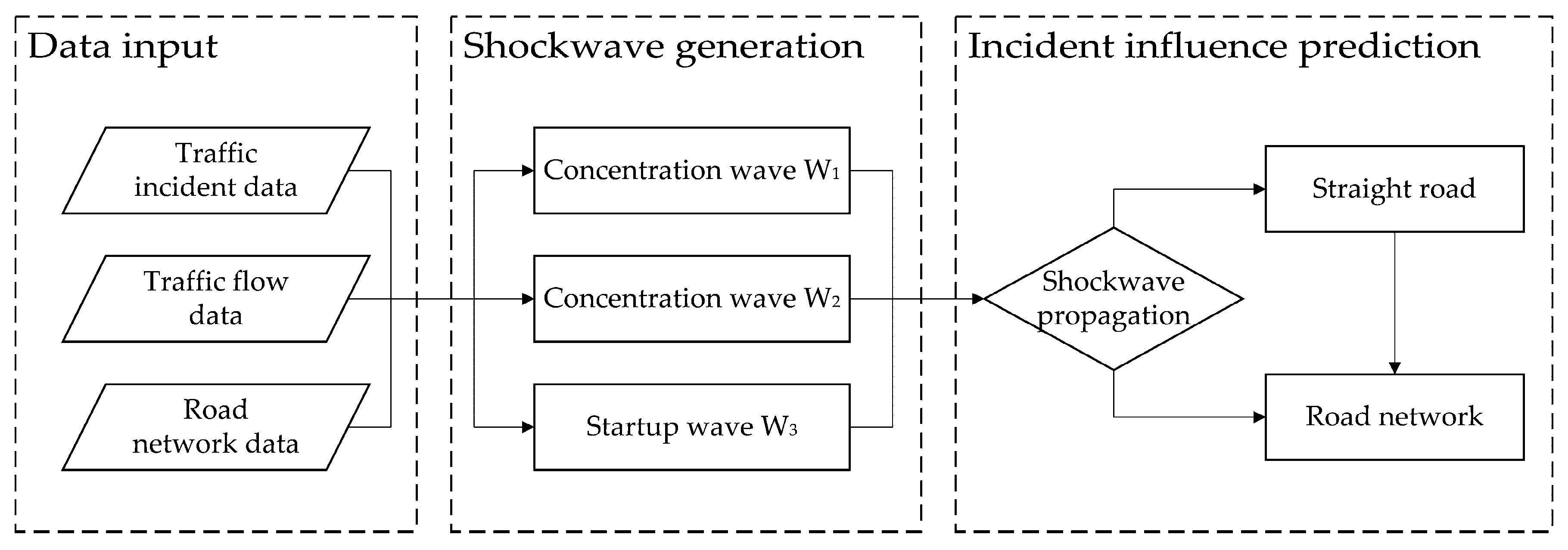
The proposed incident influence model contains three main parts: data input, shockwave generation, and incident influence prediction (Figure 1). The main components of the input data are introduced in detail in Section 2.1.
After an incident occurs, a shockwave is generated and propagates along the road. Two other shockwaves are also formed at the time when the police arrive and the incident is cleared. These are discussed in Section 2.2.
The propagation and superposition of shockwaves leads to congestion dissemination along the road network. Two situations, including the straight road prediction model and the road network prediction model, are proposed based on the different shockwaves, traffic flow, and the GIS road network. These two models are introduced in detail in Section 2.3.2 and Section 2.3.3.
2.1. Input of Incident Prediction Model
Generally, the main factors affecting congestion in a road include incidents, traffic flow, and road actuality [23]. Therefore, in this paper, the main parameters input into the prediction model contained three main parts: traffic incident information, traffic flow, and road network data (Table 1). Traffic incident information and traffic flow data can be collected from the traffic administration department of the government, while the road network data can be obtained from the GIS database.
The traffic incident data are comprised of the location, number of lanes blocked, response time, and clearance time. The location is recorded with the road name and mileage. The number of lanes blocked represents how many lanes are blocked by the incident. The response time is the period from the occurrence of the incident to the arrival of the police; the clearance time is the incident-clearing period, during which the police remove the incident-involved vehicles. The traffic flow data, which describe the vehicles passed per hour on the road of interest, is obtained in real-time from traffic cameras or coils [29]. The road network data are obtained from a GIS dataset containing information regarding each road section, including the road length () and number of lanes (). The speed limit (), road capacity per lane (), and jam density () are determined by the road design and the hierarchy of the network.
2.2. Shockwave Generation Related with Traffic Incidents
In this paper, a traffic incident refers to unexpected disruptive accidents on road networks (e.g., vehicle collisions) that require police interruption of traffic. In this situation, shockwaves will always be generated after the incident occurs and during incident clearance due to the discontinuity of traffic density (or flow) between two traffic states [30]. We assume that three shockwaves are generated after the incident: the concentration wave () occurring upon the accident, the concentration wave () upon the arrival of the police, and the startup wave () upon clearance.
Figure 2 illustrates the formation and propagation of shockwaves on homogenous adjacent road sections, where roads have the same width and number of lanes. The left part of this figure shows the location of the incident and the road sections and nodes. The time axis starts upon the occurrence of the incident (); the mileage axis is downward, and shockwaves propagate upstream. During the response period, the incident blocks some of the lanes, which reduces the traffic capacity and forms a concentration wave () that induces traffic congestion. During the clearance period (), the police block additional lanes (sometimes even the entire road section), and another concentration wave () is formed. After full clearance of the incident (), a startup wave () is formed. The propagation of indicates the dissipation of the incident’s influence. When shockwaves propagate to the same location (points M and N), they superpose with each other. The superposition between two concentration waves generates another concentration wave, while the superposition between a concentration wave and a startup wave indicates the end of the propagation.
The speed of the shockwaves () can be calculated using Equation (1) [17,31] where q is the average flow; k is the average traffic density; and the subscripts and denote the traffic states (the average flow and density, respectively):
In practice, the average density () is challenging to obtain; thus, a functional relationship is used to obtain the density from the average flow [32]. The function also determines the speed of each shockwave. In particular, the speed of startup waves is a constant related to the speed limit of the road [33], and the speed has been shown to be greater than any concentration waves [34]. Therefore, the following startup wave will definitely catch up with the previous concentration waves, which means that the influence of the incident will not be infinite.
2.3. Incident Influence Prediction Model
This subsection describes the basic prediction model for straight roads and the model for road networks. The prediction model for a straight road was first proposed to describe the propagation on a series of adjacent road sections, which is an essential part of a road network. However, after the shockwave propagates to the intersections of a road network, the straight road prediction model must be extended due to the widespread nature of shockwaves. Thus, the prediction model for a road network is proposed, which can accommodate the propagation behavior of shockwaves at intersections.
2.3.1. Derivation of Shockwave Superposition
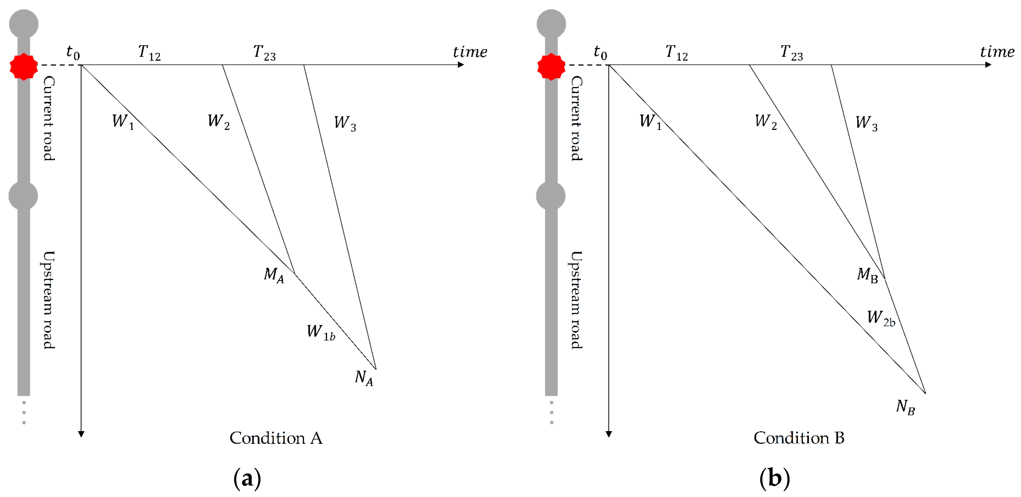
The phenomenon of Figure 2 can be extended to two conditions by the speed of the shockwaves, as shown in Figure 3. If superposes on at and forms a new concentration wave , we obtain Condition A; if superposes on at and forms a new startup wave , we obtain Condition B. The speed of and can also be determined by Equation (1).
The conditions illustrated in Figure 3 represent the basis of shockwave propagation, with the assumption that the adjacent road sections are homogenous and the nodes are disregarded. The time and location that the superposition occurs in Condition A and B were derived first.
Given the speed of each shockwave , and ; the occurrence time ; the response time ; and the clearance time , we first evaluated the condition by assuming that superposes on at ) and superposes on at ), where:
when , Condition A pertains; otherwise, Condition B pertains.
In Condition A, is formed after , and the propagation of shockwaves ends at , where superimposes on . For Condition B, is formed after , and the propagation of shockwaves ends at , where superposes on . and are the duration time and maximum influence length of the incident, respectively, and can be calculated using Equations (6)–(9):
2.3.2. Prediction Model for Straight Roads
The prediction model for straight roads predicts the incident influence on a series of adjacent road sections. The model calculates the time and location at which the superposition occurs and further outputs the influence. The shockwaves are constructed using Equation (1), where refers to the real-time traffic flow of current road sections; and is the capacity after the incident or police interruption.
In fact, the adjacent road sections differ in width and capacity, and the propagation may not end within a single road section; thus, shockwaves, together with their intervals, are recalculated when they propagate to the upstream road section.
These intervals contain the following.
- The incoming moment of the first shockwave on the upstream road section.
- The interval of the two concentration waves on the upstream road section.
- The interval of the concentration and startup wave on the upstream road section.
Considering the road length (), the two conditions illustrated in Figure 3 are further separated into four sub-conditions, A1, A2, B1, and B2, which are based on the location of the superposition between each shockwave (on the current or upstream road section). The results of the evaluation are listed in Table 2, and the time-mileage illustrations of each sub-condition are shown in Figure 4.
Conditions A1 and B1 represent no superposition on the current road section, and three shockwaves propagate to the upstream road section. Conditions A2 and B2 involve superposition on the current road section, and only two shockwaves propagate to the upstream road section; therefore, only and are derived.
The overall procedure of calculation can be implemented recursively (Figure 5). The condition of the current road section is first determined by the input, then by and . Regarding each sub-condition, the condition of the upstream road section is then determined by considering the road length and Equations (2)–(9).
Table 3 presents the parameters () of the upstream road section under each condition of continuous propagation. After the recursive calculation, the duration time is output as ; the maximum influence length is , the longest path along which the shockwave propagates.
2.3.3. Prediction Model for Road Networks
Intersections should be carefully considered when the model is implemented on urban road networks because the propagation of shockwaves changes at intersections, overpasses, and ramps. The traffic flow that moves straight ahead until turning at an intersection has a certain ratio, and a shockwave at the turning point slows down after crossing an intersection because not all vehicles enter the queue. In addition, traffic lights at intersections also affect propagation.
Figure 6a describes the incident queuing propagation at an intersection where the turning road is not fully blocked because vehicles are taking turns queuing at the turning lane. In extreme cases (Figure 6b), the turning road is fully blocked only if the propagation of the queue affects the lane-changing behavior of vehicles going straight; thus, more vehicles enter the queue [35].
Regarding the prediction model, the phenomena is abstracted. When a shockwave propagates to an intersection, different factors of shockwave speed are set in relation to the straight-going and turning roads. These factors are calibrated according to the amount of traffic flow to different destinations [18], and the effective green time at intersections [36]. We calibrated the straight factor and turning factor to be 1.1 and 0.3, respectively, for the road network of Shanghai. As a result, shockwaves to the straight direction accelerate since the intersection interrupts traffic flow and a majority of the traffic flow comes from the straight direction; shockwaves to turning directions decelerate as a small portion of traffic flow come from turning directions. Subsequently, if the influence length of the turning road section is less than a certain threshold, the influence of the turning road section is negligible, as shown in Figure 6a. The threshold is related to the functional length [37] of an intersection, which can be acquired from the road network data. In contrast, when the influence length becomes greater than the threshold, the shockwaves accelerate, indicating that more vehicles enter the queue and that the turning road is fully congested. The threshold is determined by the road hierarchy together with the length of the wide section of the intersection.
3. Case Study
3.1. Case Data
The case data used in this paper is comprised of road network data, traffic flow data, and incident data, all of which were provided by the traffic administration department of the government.
Two typical traffic incidents were selected to evaluate the proposed model. The basic information of the two incidents and their relative roads are shown in Table 4. To describe the traffic information around the incident location, the ratio of the volume demand to the capacity (V/C ratio) was used to describe the traffic volume [38]. A large V/C ratio indicated high traffic volume relative to the road capacity.
The first case was a two-car collision occurring on 1 July 2014 at 13:35 on Siping Road where one of the two lanes was blocked by the incident. The police arrived approximately within 5 min and blocked the other lane for 10 min. The V/C ratio was 0.45.
The second case was also a two-car collision that blocked one of three lanes and occurred during the evening peak on 3 March 2014 at 18:22 on Lujiabang Road. The police arrived after 380 s and blocked one additional lane for 410 s. The V/C ratio at that time was 0.7.
3.2. Incident Influence Prediction and Accuracy Evaluation
3.2.1. Incident Influence Prediction Result
The basic information of the two incidents and the relative road information were introduced into the proposed model separately. To compare the influenced roads at different timestamps, the spatiotemporal influence scopes were exported, as shown in Figure 7.
According to Figure 7, after the incidents occurred, the road was congested along the upstream direction due to the first shockwave; see 300 s in Case A and 250 s in Case B. After the police arrived and blocked additional lanes, the second shockwave formed and was superposed on the first shockwave. Therefore, the congested scope was extended during this period; see 600 s and 900 s in Case A, and 500 s and 750 s in Case B. After the clearance of the incidents, the third shockwave was formed and propagated; thus, some of the relative roads returned to an uncongested state. However, other roads—where the third shockwave had yet to be propagated—were still in a congested state, e.g., at 1000 s in Case A and Case B.
3.2.2. Accuracy Evaluation
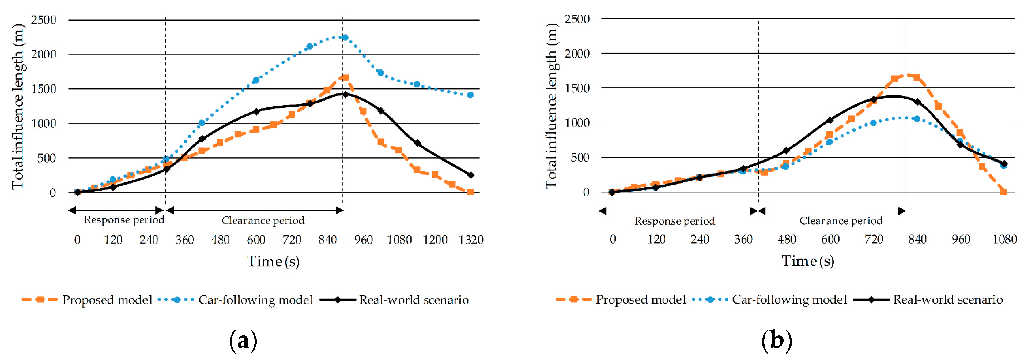
To evaluate the accuracy of the proposed model, the congestion state of the main influenced road was compared with the traffic simulation model and the actual traffic monitoring data. The traffic simulation model used was a car-following model proposed by software VISSIM [39]. The model was proposed by Wiedemann [40] and calibrated with the technique described by Yang et al. [41]. Traffic flow was simulated through dynamic assignment [42] that determined the amount and routing of the simulated vehicles. Real traffic monitoring data of both cases were collected by traffic cameras on surrounding road networks at that time. The congestion length of the road was then manually estimated and taken as the real-world value. Therefore, the influence length was obtained using the car-following model and through traffic monitoring. Figure 8 illustrates the comparison of the total influence length predicted by the proposed model, the car-following model, and the real-world case.
The tendencies predicted by the proposed model and the car-following model were similar to that of the real-world case captured by traffic monitoring data. During the response period, the influence length was essentially the same, demonstrating that both the proposed method and the car-following model worked well during the response period. The cumulative influence length increased during the clearance period as the police blocked an additional lane. The influence length reached its maximum at the end of the clearance period. Relative to the actual data, the proposed models predicted a larger maximum influence length in both cases. The car-following model predicted a larger influence scope in Case A, but a smaller influence length in Case B.
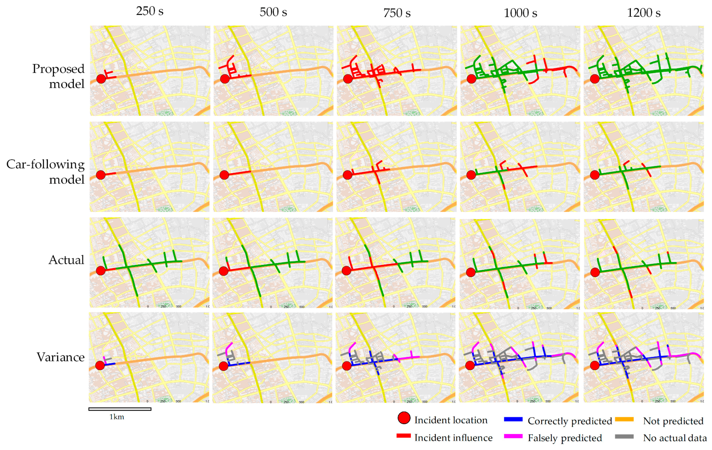
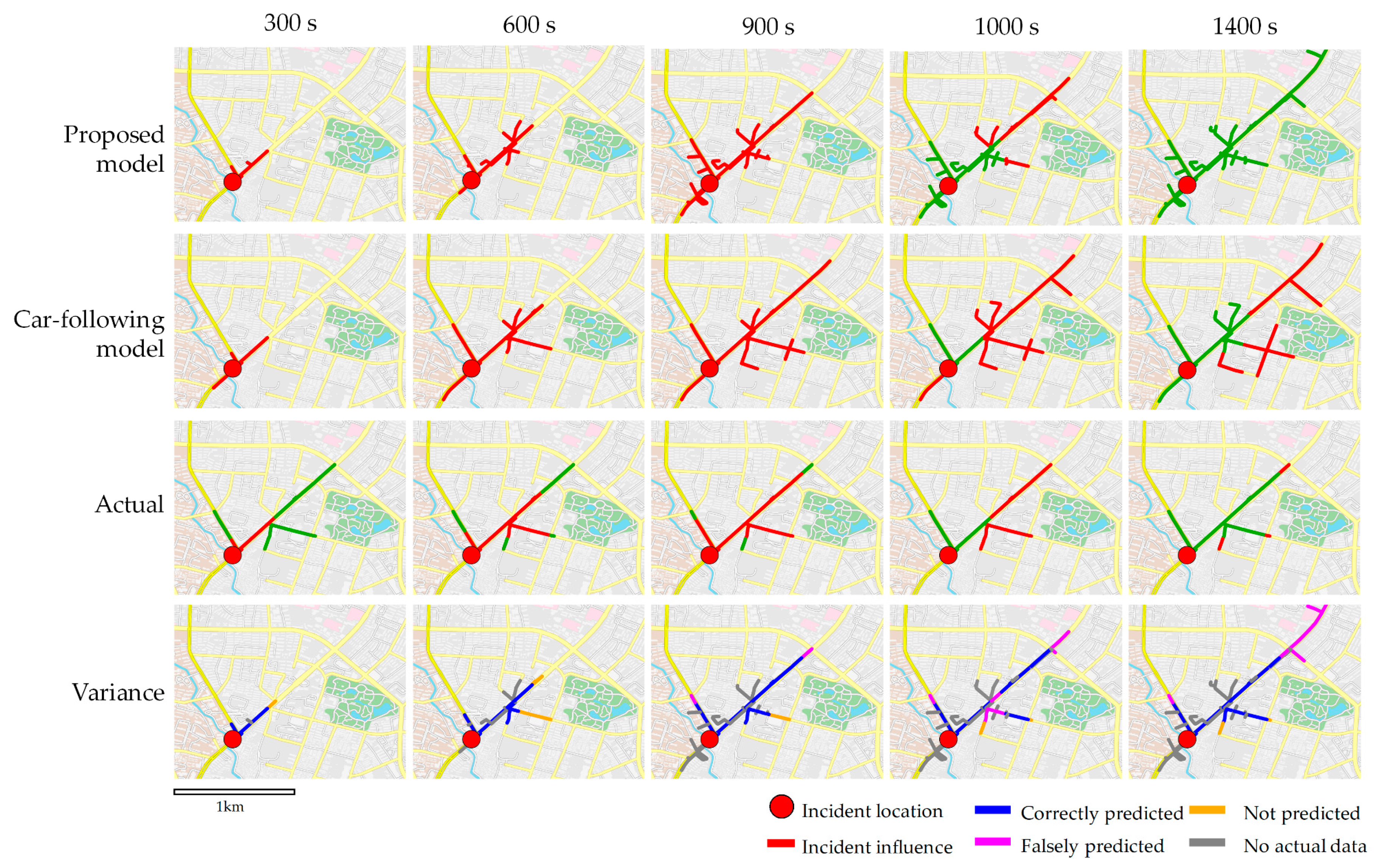
The spatiotemporal results of the two cases were also compared in congestion diagrams and variance diagrams at certain timestamps, as shown in Figure 9 and Figure 10 where ‘not predicted’ indicates the roads that were under influence, but unpredicted; ‘falsely predicted’ means the opposite; and ‘no actual data’ means that actual data were not collected as traffic monitoring was not conducted.
In the actual scenario, the spatial distribution of the incident influence was larger on the main road where the incident occurred, but smaller on the surrounding turning roads. This phenomenon was predicted by both models. The proposed model in the first row covered more minor roads than the car-following model and the actual scenario, but the influence on those collector roads was not included in the evaluation. The last row of both Figure 9 and Figure 10 show the variance between the proposed model and the real-world scenario. In both cases, the proposed model provided a more accurate prediction on the main road than on the minor roads. However, in Case B—with a denser surrounding road network—a larger number of false predictions arose after propagation through several intersections. Additionally, the car-following model predicted a larger scope in Case A, particularly on collector roads several intersections away. In contrast, the influence scope predicted by the car-following model was smaller than that of the real-world scenario in Case B. The proportion of road length that was correctly predicted/not predicted/falsely predicted was further collected by statistics and is listed in Table 5.
Table 5 quantifies the evaluation of the proposed model in the ‘variance’ row of Figure 10 by listing the proportion of different evaluation results. For Case A, the proposed model featured over 70% of accuracy over the congestion process, falling to 60% during the dissipation. Though the proportion of ‘not predicted’ decreased over time, the false predictions increased, particularly during dissipation. The accuracy fell to 60%, and the number of false predictions rose in Case B, which involved a high-density road network downtown.
According to Table 5, the overall accuracy of the proposed model was higher over the congestion process, but decreased during dissipation. The shockwave model introduced in this paper is macroscopic; it abstracts driving behaviors including lane-changing, acceleration, and deceleration. Thus, a decrease in accuracy was expected over the dissipation process and during congestion processes where lanes were not fully blocked. The lane-changing behavior slowed down the dissipation, and the behavior of changing to the free lane slowed down the congestion. These effects may explain the overprediction of the proposed model. Additionally, the high-density collector road network downtown in Case B exhibited increased uncertainty of traffic, making the impact of non-motorized vehicles, pedestrians, and curb parking non-negligible.
3.2.3. Computational Efficiency Evaluation
The efficiency of the proposed model was also evaluated by comparing the computation time with the car-following model in the two cases above. The selected verification platform was a computer with a 2.2 GHz CPU and 8 GB RAM. The computation times for both cases are listed in Table 6.
4. Conclusions and Future Work
This paper presented a dynamic spatiotemporal analysis model predicting the influence of traffic incidents with the assistance of a GIS database and knowledge of the road network. This model used a traffic shockwave model, and different superposition situations of shockwaves were proposed for both straight roads and road networks. This approach ensures that the influence is transferred along the upstream of the road, and then propagates through turns to minor roads.
Two typical incidents occurring in Shanghai were selected to verify the proposed model and compare it against the car-following model and actual monitoring data. The results showed that the proposed model successfully predicted the congestion of a main road in the response period and that the degree of false prediction increased during the clearance period. Relative to the actual monitoring data, the proposed model generally reached an accuracy of over 60%. Moreover, the proposed model required fewer computation resources and could be used to predict a broader set of road hierarchies than the car-following model.
The novelty of the proposed model is that the shockwave traffic model can be successfully integrated with GIS spatiotemporal analysis to predict the congestion situation for incidents and for different road hierarchies. Compared with data-driven methods like those in [2,3,4], only few historical data and dynamic parameters are required for the model, ensuring that the proposed model could be used in most traffic prediction systems and ITSs. Compared with the approach described in [26], this method describes the influence of traffic incidents not only on freeways, but also on surface streets using dynamic incident data. The propagation of shockwaves through intersections was also tackled by considering the different behaviors of shockwaves towards straight and turning roads.
The proposed shockwave model simplifies the process procedure of driving behavior and collector road networks. In the model, the lane-changing behavior under the context of congestion and dissipation was abstracted into the propagation of shockwaves. However, this idealization may lead to less accurate prediction, as more complex traffic phenomena on downtown high-density road networks are omitted. In future work, we plan to expand the model to consider more complex scenarios to achieve more precise results such as considering the perturbation of shockwaves caused by lane changing on collector roads.
In this paper, the traffic flow and GIS road network data were provided by the Traffic Administration Department of the Chinese Government. However, the actual traffic flow changes daily, which will decrease the accuracy of the proposed model. The accuracy can be restored if the real-time traffic flow of a road is imported to the proposed model.
Another limitation of the proposed model is that the incident was assumed to require police intervention. However, some incidents involving lower economic losses and unambiguous responsibility are non-disruptive according to local traffic management laws. Therefore, the response time and clearance time of the model will not be provided. In this situation, the incident location can be automatically detected, and the clearance time can be estimated by the ITS of the city.
Acknowledgments
This study was supported by the National Science and Technology Major Program (grant No. 2016YFB0502102 and No. 2016YFB0502104), National Natural Science Foundation of China (grant No. 51308409) and the Fundamental Research Funds for the Central Universities of China. The authors thank the Shanghai Road Administration Bureau for providing traffic data.
Author Contributions
Chun Liu conceived the research idea. Shuhang Zhang, and Qiang Fu derived the model. Chun Liu, Shuhang Zhang, and Hangbin Wu designed the experiments. Shuhang Zhang analyzed the result and wrote the manuscript. Chun Liu, Hangbin Wu, and Qiang Fu edited the manuscript.
Conflicts of Interest
The authors declare no conflict of interest.
References
- Chou, C. Understanding the Impact of Incidents and Incident Management Programs on Freeway Mobility and Safety; University of Maryland: College Park, MD, USA, 2010. [Google Scholar]
- Pan, B.; Demiryurek, U.; Gupta, C.; Shahabi, C. Forecasting spatiotemporal impact of traffic incidents for next-generation navigation systems. Knowl. Inf. Syst. 2015, 45, 75–104. [Google Scholar] [CrossRef]
- Miller, M.; Gupta, C. Mining traffic incidents to forecast impact. In Proceedings of the ACM SIGKDD International Workshop on Urban Computing, Beijing, China, 12–16 August 2012; pp. 33–40. [Google Scholar]
- Xu, J.; Deng, D.; Demiryurek, U.; Shahabi, C.; van der Schaar, M. Mining the situation: Spatiotemporal traffic prediction with big data. IEEE J. Sel. Top. Signal Process. 2015, 9, 702–715. [Google Scholar] [CrossRef]
- Goodchild, M.F. GIS and Transportation: Status and Challenges. Geoinformatica 2000, 4, 127–139. [Google Scholar] [CrossRef]
- Peng, G.; Sun, Y. Study on Urban Traffic Incident GIS-T Data Model. In Proceedings of the International Workshop on Education Technology and Training, 2008. and 2008 International Workshop on Geoscience and Remote Sensing, Shanghai, China, 21–22 December 2008; pp. 149–152. [Google Scholar]
- Chen, S.; Tan, J.; Claramunt, C.; Ray, C. Multi-scale and multi-modal GIS-T data model. J. Transp. Geogr. 2011, 19, 147–161. [Google Scholar] [CrossRef]
- Chang, L.; Chen, W. Data mining of tree-based models to analyze freeway accident frequency. J. Saf. Res. 2005, 36, 365–375. [Google Scholar] [CrossRef] [PubMed]
- Kundakci, E.; Tuydesyaman, H. Understanding the Distribution of Traffic Accident Hot Spots in Urban Regions. In Proceedings of the Transportation Research Board 93rd Annual Meeting, Washington, DC, USA, 12–16 January 2014. [Google Scholar]
- Appert, M.; Laurent, C. Measuring urban road network vulnerability using graph theory: The case of Montpellier’s road network. J. Rural Probl. 2007, 47, 66–71. [Google Scholar]
- Pollak, K.; Peled, A.; Hakkert, S. Geo-Based Statistical Models for Vulnerability Prediction of Highway Network Segments. ISPRS Int. J. Geo-Inf. 2014, 3, 619–637. [Google Scholar] [CrossRef]
- Anbaroglu, B.; Heydecker, B.; Cheng, T. Spatio-temporal clustering for non-recurrent traffic congestion detection on urban road networks. Transp. Res. Part C Emerg. Technol. 2014, 48, 47–65. [Google Scholar] [CrossRef]
- Wu, H.; Liu, C.; Wang, J.; Yao, L.; Zhang, S.; Li, Y.; Li, Z.; Liu, C.; Fang, S. ATSSS: An Active Traffic Safety Service System in Pudong New District, Shanghai, China. In Progress in Location-Based Services 2014; Springer: Berlin, Germany, 2015; pp. 239–253. [Google Scholar]
- Roberg-Orenstein, P.; Abbess, C.; Wright, C. Traffic jam simulation. J. Maps 2007, 3, 107–121. [Google Scholar] [CrossRef]
- Long, J.; Gao, Z.; Zhao, X.; Lian, A.; Orenstein, P. Urban traffic jam simulation based on the cell transmission model. Netw. Spat. Econ. 2011, 11, 43–64. [Google Scholar] [CrossRef]
- Brackstone, M.; Mcdonald, M. Car-following: A historical review. Transp. Res. Part F Traffic Psychol. Behav. 1999, 2, 181–196. [Google Scholar] [CrossRef]
- Lighthill, M.J.; Whitham, G.B. On kinematic waves. II. A theory of traffic flow on long crowded roads. In Proceedings of the Royal Society of London A: Mathematical, Physical and Engineering Sciences; The Royal Society: London, UK, 1955; pp. 317–345. [Google Scholar]
- Zhou, X.; Taylor, J. DTALite: A queue-based mesoscopic traffic simulator for fast model evaluation and calibration. Cogent Eng. 2014, 1, 961345. [Google Scholar] [CrossRef]
- Qu, Y.; Zhou, X. Large-scale dynamic transportation network simulation: A space-time-event parallel computing approach. Transp. Res. Part Emerg. Technol. 2017, 75, 1–16. [Google Scholar] [CrossRef]
- Imprialou, M.M.; Orfanou, F.P.; Vlahogianni, E.I.; Karlaftis, M.G. Methods for Defining Spatiotemporal Influence Areas and Secondary Incident Detection in Freeways. J. Transp. Eng. 2014, 140, 70–80. [Google Scholar] [CrossRef]
- Park, H.; Haghani, A. Real-time prediction of secondary incident occurrences using vehicle probe data. Transp. Res. Part C Emerg. Technol. 2016, 70, 69–85. [Google Scholar] [CrossRef]
- Demiroluk, S.; Ozbay, K. Adaptive learning in bayesian networks for incident duration prediction. Transp. Res. Rec. J. Transp. Res. Board 2014, 2460, 77–85. [Google Scholar] [CrossRef]
- Chung, Y.; Recker, W.W. A Methodological Approach for Estimating Temporal and Spatial Extent of Delays Caused by Freeway Accidents. IEEE Trans. Intell. Transp. 2012, 13, 1454–1461. [Google Scholar] [CrossRef]
- Chung, Y.; Recker, W.W. Frailty Models for the Estimation of Spatiotemporally Maximum Congested Impact Information on Freeway Accidents. IEEE Trans. Intell. Transp. 2015, 16, 2104–2112. [Google Scholar] [CrossRef]
- Khattak, A.; Wang, X.; Zhang, H. Incident management integration tool: Dynamically predicting incident durations, secondary incident occurrence and incident delays. IET Intell. Transp. Syst. 2012, 6, 204–214. [Google Scholar] [CrossRef]
- Sarker, A.A.; Naimi, A.; Mishra, S.; Golias, M.M.; Freeze, P.B. Development of a Secondary Crash Identification Algorithm and occurrence pattern determination in large scale multi-facility transportation network. Transp. Res. Part C Emerg. Technol. 2015, 60, 142–160. [Google Scholar] [CrossRef]
- Shaw, S. Geographic information systems for transportation: From a static past to a dynamic future. Ann. GIS 2010, 16, 129–140. [Google Scholar] [CrossRef]
- Loidl, M.; Wallentin, G.; Cyganski, R.; Graser, A.; Scholz, J.; Haslauer, E. GIS and Transport Modeling—Strengthening the Spatial Perspective. ISPRS Int. J. Geo-Inf. 2016, 5, 84. [Google Scholar] [CrossRef]
- Kunzler, M.; Udd, E.; Taylor, T.; Kunzler, W. Traffic monitoring using fiber optic grating sensors on the I-84 freeway and future uses in WIM. In Proceedings of the International Society for Optics and Photonics, Troutdale, OR, USA, 20 November 2003; pp. 122–127. [Google Scholar]
- Wada, K.; Ohata, T.; Kobayashi, K.; Kuwahara, M. Traffic Measurements on Signalized Arterials from Vehicle Trajectories. Interdiscip. Inf. Sci. 2015, 21, 77–85. [Google Scholar] [CrossRef]
- Logghe, S.; Immers, L.H. Multi-class kinematic wave theory of traffic flow. Transp. Res. Part B Methodol. 2008, 42, 523–541. [Google Scholar] [CrossRef]
- Newell, G.F. A simplified theory of kinematic waves in highway traffic, part II: Queueing at freeway bottlenecks. Transp. Res. Part B Methodol. 1993, 27, 289–303. [Google Scholar] [CrossRef]
- Helbing, D. Fundamentals of Traffic Flow. Phys. Rev. E Stat. Phys. Plasmas Fluid. Relat. Interdiscip. Top. 1998, 55, 3735–3738. [Google Scholar] [CrossRef]
- Jabari, S.E.; Zheng, J.; Liu, H.X. A probabilistic stationary speed–density relation based on Newell’s simplified car-following model. Transp. Res. Part B Methodol. 2014, 68, 205–223. [Google Scholar] [CrossRef]
- Wright, C.; Roberg, P. The conceptual structure of traffic jams. Transp. Polic. 1998, 5, 23–35. [Google Scholar] [CrossRef]
- Zlatkovic, M.; Zhou, X. Integration of signal timing estimation model and dynamic traffic assignment in feedback loops: System design and case study. J. Adv. Transp. 2015, 49, 683–699. [Google Scholar] [CrossRef]
- Chandler, B.E.; Myers, M.C.; Atkinson, J.E.; Bryer, T.E.; Retting, R.; Smithline, J.; Trim, J.; Wojtkiewicz, P.; Thomas, G.B.; Venglar, S.P.; et al. Signalized Intersections Informational Guide; FHWA-SA-13-027; U.S. Department of Transportation: Washington, DC, USA, 2013.
- Zhou, M.; Sisiopiku, V. Relationship between Volume-to-Capacity Ratios and Accident Rates. Transp. Res. Rec. J. Transp. Res. Board 1997, 1581, 47–52. [Google Scholar] [CrossRef]
- PTV AG. VISSIM 5.40: User Manual; PTV Group: Karlsruhe, Germany, 2011. [Google Scholar]
- Wiedemann, R. Simulation des Straßenverkehrsflusses; Institut für Verkehrswesen der Universität Karlsruhe: Karlsruhe, Germany, 1974. [Google Scholar]
- Yang, H.; Han, S.; Chen, X. Parameter calibration and application for the Vissim simulation model. Urban Transp. China 2006, 06, 22–25. [Google Scholar]
- Gomes, G.; May, A.; Horowitz, R. Congested freeway microsimulation model using VISSIM. Transp. Res. Rec. J. Transp. Res. Board 2004, 1876, 71–81. [Google Scholar] [CrossRef]
Figure 1.
Schematic illustration of the spatiotemporal influence prediction model for a traffic incident.
Figure 1.
Schematic illustration of the spatiotemporal influence prediction model for a traffic incident.

Figure 2.
Schematic diagram of the formation, propagation, and superposition of shockwaves. The illustration of road sections is on the left; the propagation and superposition of shockwaves is on the right.
Figure 2.
Schematic diagram of the formation, propagation, and superposition of shockwaves. The illustration of road sections is on the left; the propagation and superposition of shockwaves is on the right.
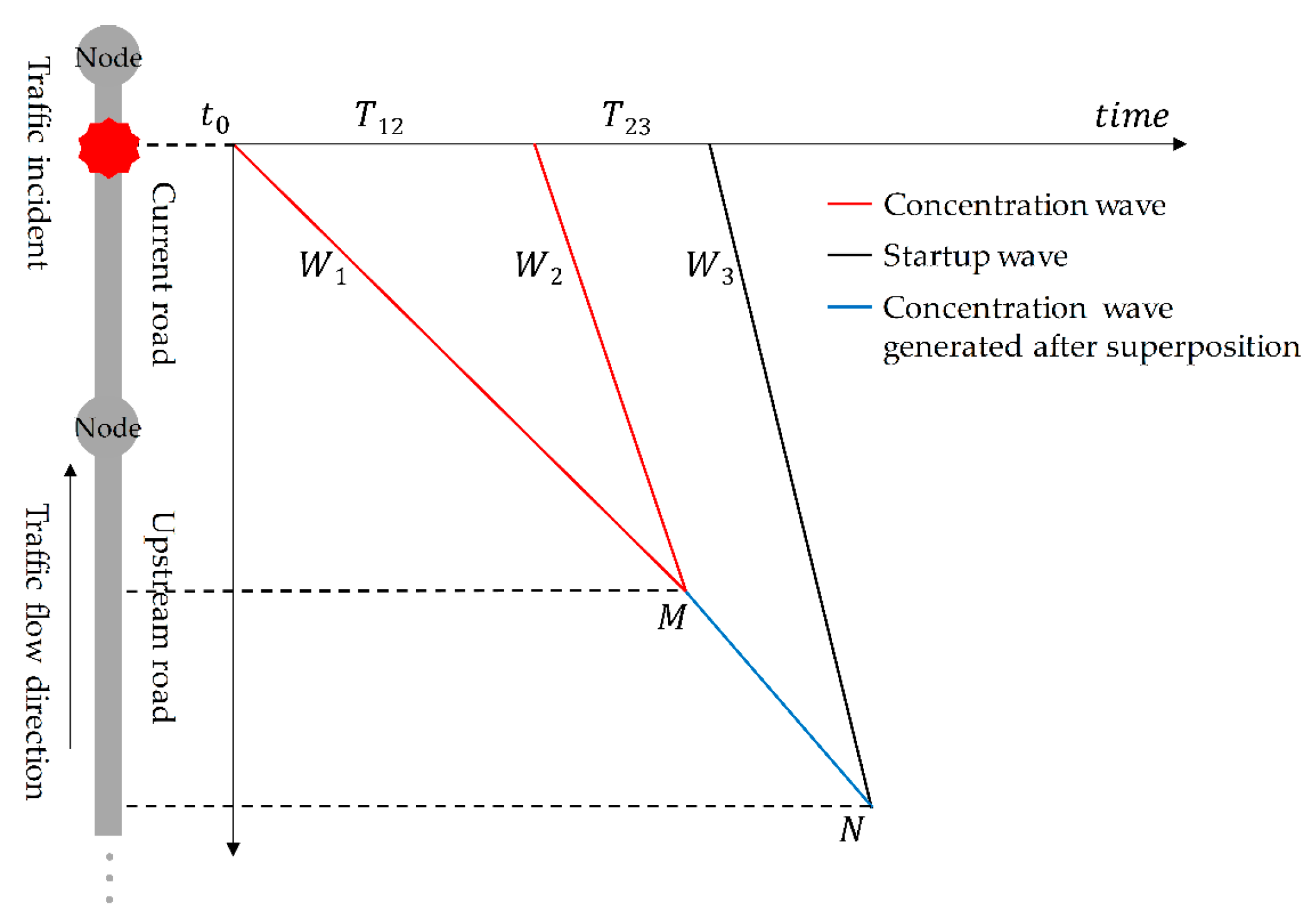
Figure 3.
Basic conditions of shockwave superposition: (a) Condition A; and (b) Condition B.

Figure 4.
Propagation conditions: (a) Condition A1; (b) Condition B1; (c) Condition A2; and (d) Condition B2. The illustrations of road sections on the left are similar to that in Figure 2. The current road section is on the white background, and the upstream road section is on the gray background. The dashed line ‘’ represents the length of the current road section.
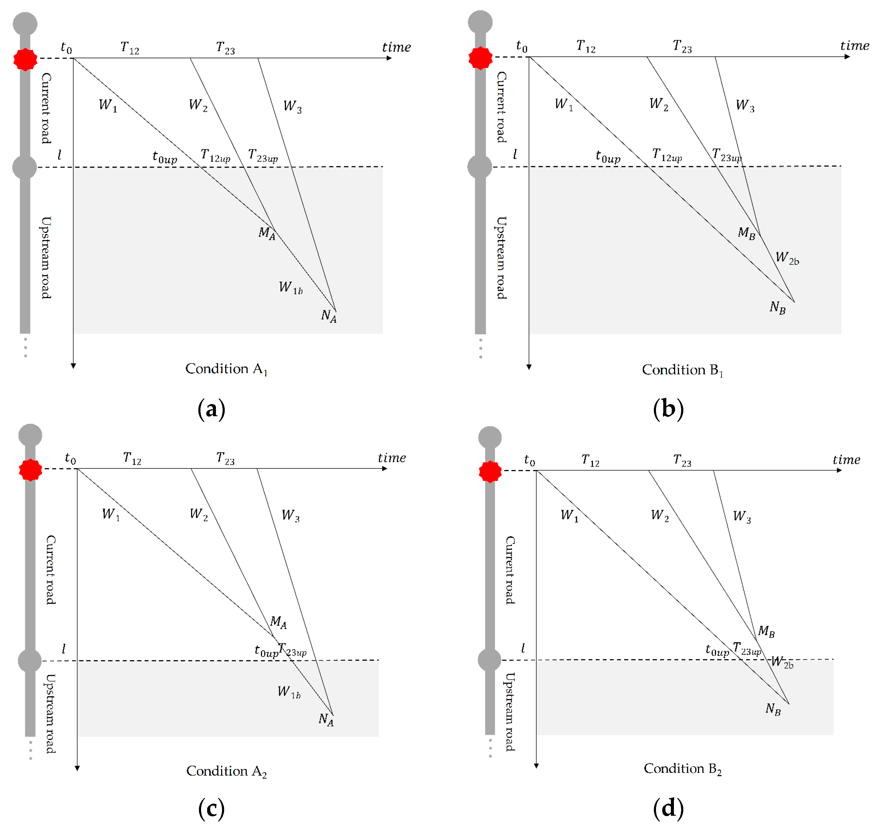
Figure 5.
Overall procedure of condition evaluation of current and upstream road sections.
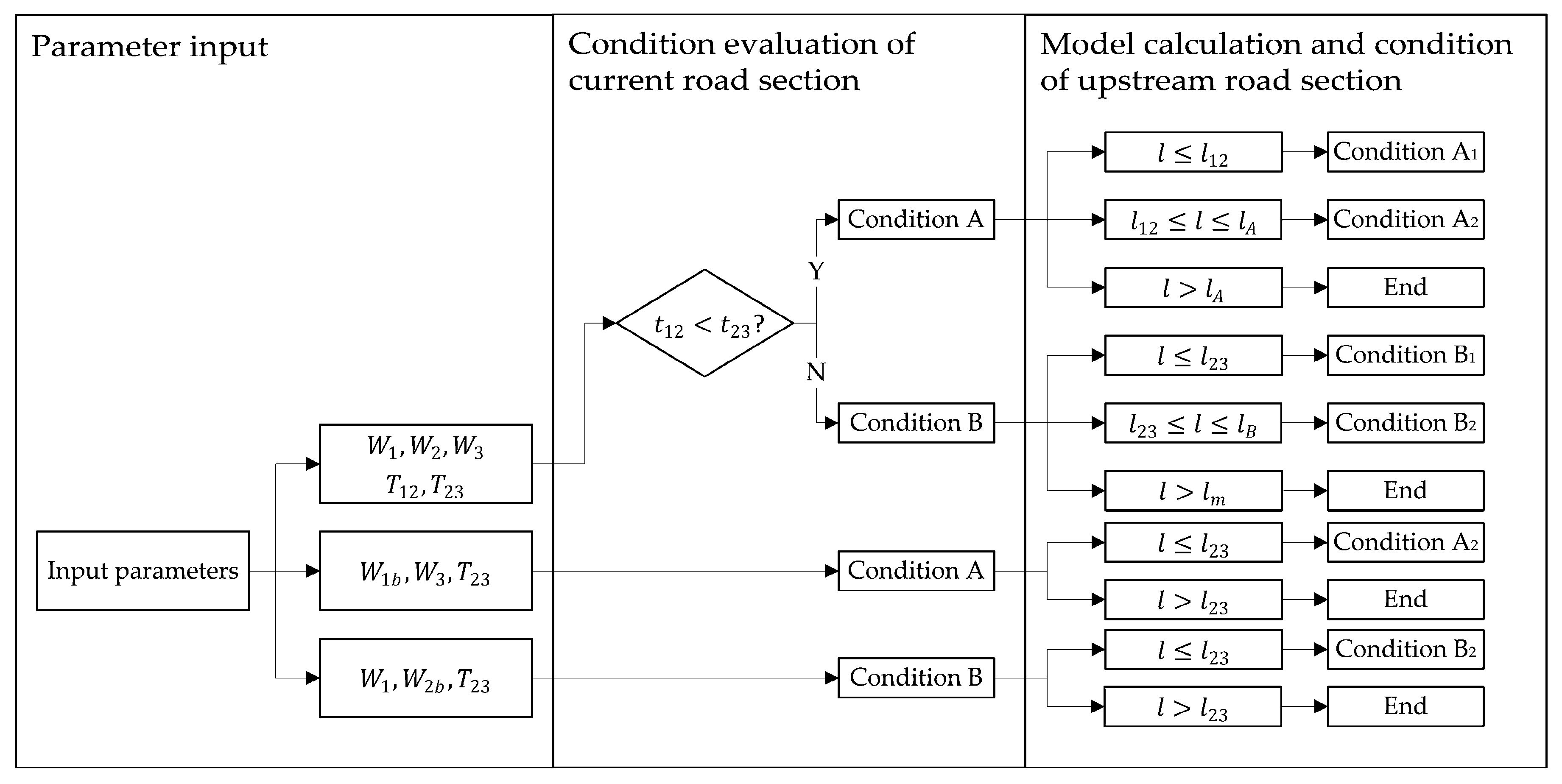
Figure 6.
(a) Queuing propagation at an intersection. Vehicles drawn in different colors take different trajectories; (b) Interference of vehicles taking turns and going straight.
Figure 6.
(a) Queuing propagation at an intersection. Vehicles drawn in different colors take different trajectories; (b) Interference of vehicles taking turns and going straight.
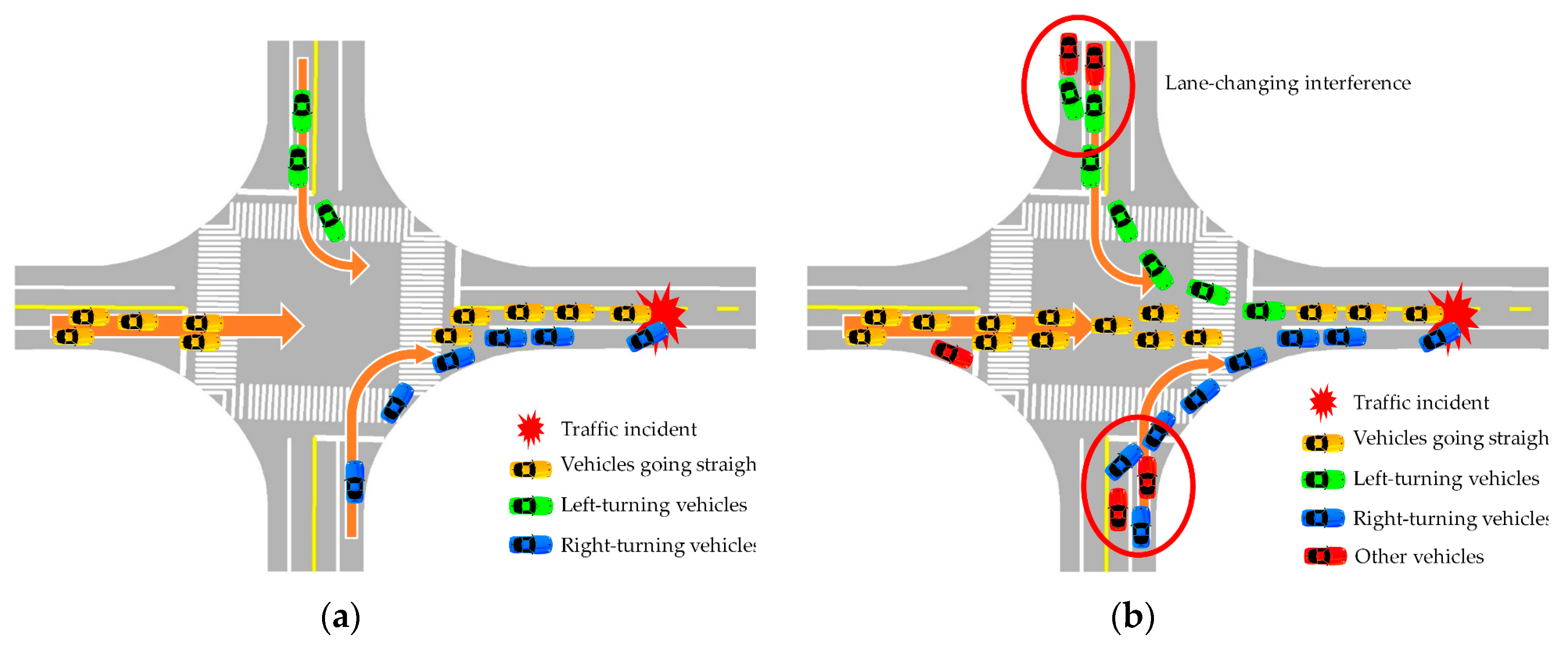
Figure 7.
Spatiotemporal influence scope of two cases at different timestamps. The roads marked in red are congested, and the roads whose startup shockwave has already passed are free and marked in green.
Figure 7.
Spatiotemporal influence scope of two cases at different timestamps. The roads marked in red are congested, and the roads whose startup shockwave has already passed are free and marked in green.
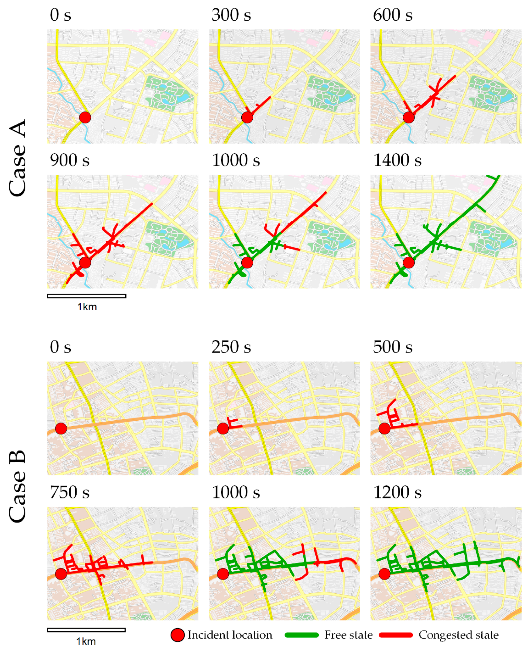
Figure 8.
Total influence length comparison between the proposed model, car-following model, and real-world scenario of (a) Case A; and (b) Case B.
Figure 8.
Total influence length comparison between the proposed model, car-following model, and real-world scenario of (a) Case A; and (b) Case B.

Figure 9.
Spatiotemporal diagrams comparing the result of the proposed model, car-following model and actual data for Case A. The variance between the proposed model and truth is shown in the fourth row.
Figure 9.
Spatiotemporal diagrams comparing the result of the proposed model, car-following model and actual data for Case A. The variance between the proposed model and truth is shown in the fourth row.

Figure 10.
Spatiotemporal diagrams comparing the result of the proposed model, car-following model and actual data for Case B. The variance between proposed model and truth is shown in the fourth row.
Figure 10.
Spatiotemporal diagrams comparing the result of the proposed model, car-following model and actual data for Case B. The variance between proposed model and truth is shown in the fourth row.

Table 1.
Inputs to the spatiotemporal influence prediction model from the traffic incident.
| Data Type | Parameter |
|---|---|
| Traffic incident data | Location— |
| Occurrence time— | |
| Number of lanes blocked— | |
| Response time— | |
| Clearance time— | |
| Traffic flow data | Traffic flow of each road section— |
| Road network data | Road section length— |
| Speed limit— | |
| Number of lanes— | |
| Road capacity per lane— | |
| Jam density— |
Table 2.
Evaluation of the sub-conditions of shockwave propagation.
| Condition Type | ||
|---|---|---|
| Condition A1 | Upstream road | - |
| Condition B1 | - | Upstream road |
| Condition A2 | Current road | - |
| Condition B2 | - | Current road |
Table 3.
Parameters of the upstream road section under each condition of continuous propagation.
| Condition of Current Road | Condition of Upstream Road | |||
|---|---|---|---|---|
| Condition A1 | A1 | |||
| A2 | - | |||
| Condition B1 | A1 | |||
| B2 | - | |||
| Conditions A2 and B2 | A2, B2 | - |
Table 4.
Information for selected cases.
| Description | Case A | Case B |
|---|---|---|
| Time | 1 July 2014 13:35 | 3 March 2014 18:22 |
| Type | Two-car collision | Two-car collision |
| Location | Siping Road, 50 m south of Quyang Road | Lujiabang Road, 35 m east of Zhaozhou Road |
| Police arrival time | 300 s | 380 s |
| Clearance time | 600 s | 410 s |
| Number of lanes blocked | 1 | 1 |
| Road hierarchy | Secondary arterial | Primary arterial |
| Number of lanes | 2 | 3 |
| Traffic capacity per lane | 650 veh/h | 900 veh/h |
| V/C ratio | 0.45 | 0.7 |
Table 5.
Proportion of the road length that is correctly predicted/not predicted/falsely predicted in the two cases.
Table 5.
Proportion of the road length that is correctly predicted/not predicted/falsely predicted in the two cases.
| Time | Correctly Predicted | Not Predicted | Falsely Predicted | |
|---|---|---|---|---|
| Case A | 300 s | 84.5% | 15.5% | 0.0% |
| 600 s | 74.1% | 25.9% | 0.0% | |
| 900 s | 77.6% | 6.7% | 15.7% | |
| 1000 s | 66.6% | 4.3% | 29.1% | |
| 1400 s | 61.5% | 3.6% | 34.8% | |
| Case B | 250 s | 63.3% | 0.0% | 36.7% |
| 500 s | 67.7% | 0.0% | 32.3% | |
| 750 s | 65.7% | 0.0% | 34.3% | |
| 1000 s | 64.0% | 2.1% | 33.9% | |
| 1200 s | 57.7% | 7.2% | 35.1% | |
Table 6.
Computation time comparison between the proposed model and the car-following model.
| Model | Case A | Case B |
|---|---|---|
| Proposed model | 1.98 s | 4.78 s |
| Car-following model | 38 s | 105 s |
© 2017 by the authors. Licensee MDPI, Basel, Switzerland. This article is an open access article distributed under the terms and conditions of the Creative Commons Attribution (CC BY) license (http://creativecommons.org/licenses/by/4.0/).
Share and Cite
MDPI and ACS Style
Liu, C.; Zhang, S.; Wu, H.; Fu, Q. A Dynamic Spatiotemporal Analysis Model for Traffic Incident Influence Prediction on Urban Road Networks. ISPRS Int. J. Geo-Inf. 2017, 6, 362. https://doi.org/10.3390/ijgi6110362
AMA Style
Liu C, Zhang S, Wu H, Fu Q. A Dynamic Spatiotemporal Analysis Model for Traffic Incident Influence Prediction on Urban Road Networks. ISPRS International Journal of Geo-Information. 2017; 6(11):362. https://doi.org/10.3390/ijgi6110362
Chicago/Turabian StyleLiu, Chun, Shuhang Zhang, Hangbin Wu, and Qiang Fu. 2017. "A Dynamic Spatiotemporal Analysis Model for Traffic Incident Influence Prediction on Urban Road Networks" ISPRS International Journal of Geo-Information 6, no. 11: 362. https://doi.org/10.3390/ijgi6110362
Note that from the first issue of 2016, this journal uses article numbers instead of page numbers. See further details here.