An Ensemble Model for Co-Seismic Landslide Susceptibility Using GIS and Random Forest Method


1
Division of Earth Environmental System Science, Pukyong National University, 45 Yongso–ro, Nam-gu, Busan 48513, Korea
2
Department of Geography, University of Bergen, Fosswinckelsgt. 6, 5020 Bergen, Norway
*
Author to whom correspondence should be addressed.
ISPRS Int. J. Geo-Inf. 2017, 6(11), 365; https://doi.org/10.3390/ijgi6110365
Submission received: 5 July 2017
/
Revised: 4 November 2017
/
Accepted: 13 November 2017
/
Published: 16 November 2017
Abstract
:The Mw 7.8 Gorkha earthquake of 25 April 2015 triggered thousands of landslides in the central part of the Nepal Himalayas. The main goal of this study was to generate an ensemble-based map of co-seismic landslide susceptibility in Sindhupalchowk District using model comparison and combination strands. A total of 2194 co-seismic landslides were identified and were randomly split into 1536 (~70%), to train data for establishing the model, and the remaining 658 (~30%) for the validation of the model. Frequency ratio, evidential belief function, and weight of evidence methods were applied and compared using 11 different causative factors (peak ground acceleration, epicenter proximity, fault proximity, geology, elevation, slope, plan curvature, internal relief, drainage proximity, stream power index, and topographic wetness index) to prepare the landslide susceptibility map. An ensemble of random forest was then used to overcome the various prediction limitations of the individual models. The success rates and prediction capabilities were critically compared using the area under the curve (AUC) of the receiver operating characteristic curve (ROC). By synthesizing the results of the various models into a single score, the ensemble model improved accuracy and provided considerably more realistic prediction capacities (91%) than the frequency ratio (81.2%), evidential belief function (83.5%) methods, and weight of evidence (80.1%).
1. Introduction
On 25 April 2015, a catastrophic earthquake of Mw 7.8 was struck Nepal at 06:11:26 UTC. The epicenter of the main shock was located at Barpak, (28°15′07″ N, 84°07′02″ E) in the Gorkha District, approximately 75 km east of Kathmandu. The earthquake killed more than 9000 people, and fully or partially damaged 1.1 million houses [1]. Over 400 aftershocks of ≥Mw 4 were recorded within two years after the main quake. The earthquake also triggered various mass movements [2,3], some of which caused damage, such as blocked roads and dammed rivers, and threatened infrastructures in many parts of the earthquake-affected areas with steep topography and deep valleys.
Landslides caused by earthquakes are known to be a major natural hazard, in some cases causing as much or more damage than the initial ground shaking [4], and the Gorkha earthquake was not an exception. The shock vibration around the steep mountains caused a large number of landslides and debris flows. More than 40 people were rescued from such debris flows, and over 3000 people were reported missing. The effects of co-seismic landslides were most severe in settlements around Sindhupalchowk District, causing complete destruction of 96.8% of the houses and the loss of 3550 lives [3].
Compilation of co-seismic landslides into an inventory is crucial, and statistical analyses of the spatial distribution of such landslides are significant in determining the areas most susceptible to landslides in future extreme events such as earthquakes and torrential rainfall [5]. Shaking induced by previous events might weaken slopes (by opening joints in rock masses, fracturing materials, increasing pore water pressure in soil slopes, reducing cohesion in soils, etc.). The effects can cause slopes to fail in subsequent earthquakes, even under low-intensity events. According to Papadopoulos and Plessa [6], such conditions are a possible cause of earthquake-induced landslide disasters in Greece. In recent years, several statistical methods have emerged for analyzing co-seismic landslides related to individual earthquake events [5,7,8,9]. These methods comprise causative factors (CFs) such as soil depth, slope angle, soil or rock strength index, vegetation cover, terrain roughness, moisture content, height, horizontal distance to roads, streams, etc., and peak ground acceleration (PGA) with the modified Mercalli (MM) intensity [10,11]. The scale of analysis, essential details of the susceptibility map, and the accessibility and quality of input data influence such methodologies [12,13,14,15]. Analytical problems arise when individual models act differently on the same set of data. Such differences between the results of different models can be attributed to differences in model belief and algorithms, or demand of various definite data. These drawbacks can be avoided by applying an ensemble of models for landslide susceptibility modeling, rather than the outputs from single model. Although some previous studies have assessed landslide susceptibility by comparing forecasts from multiple models, there is presently no agreed method for combining different geographical forecasts into an optimal prediction [16]. Molteni et al. [17] and Marsigli et al. [18] used different models that produced separate results, then evaluated these results independently and combined them into the best performing optimal forecast.
In this work, popular bivariate models such as the frequency ratio (FR) [19,20,21,22], evidential belief function (EBF) [22,23,24], and weight of evidence (WOE) [22,25,26,27,28,29,30] methods were used and compared. Discrepancies among the results from different modeling approaches may be due to differences in model assumptions and algorithms. These common situations led to suggest using an ensemble of models for landslide susceptibility modeling, rather than relying on outputs from a single model to guide eradication efforts [31]. A random forest (RF) classification was adopted to combine the models and produce an ensemble landslide susceptibility map. RF is an ensemble learning method of classification that combines the idea of bagging with random feature selection. It has several other advantages: (i) it does not require assumptions on the distribution of explanatory parameters; (ii) it allows for the mixed use of categorical and numerical parameters without using dummy parameters; and (iii) it can account for interactions and nonlinearities between parameters [28,29,30,31,32,33,34,35,36]. RF classification and regression methods are widely used in remote sensing for image classification [37]. This study could provide new insights into co-seismic landslide susceptibility modeling in severely landslide-affected regions where available data are rather limited and differences in scale exist.
2. Study Area
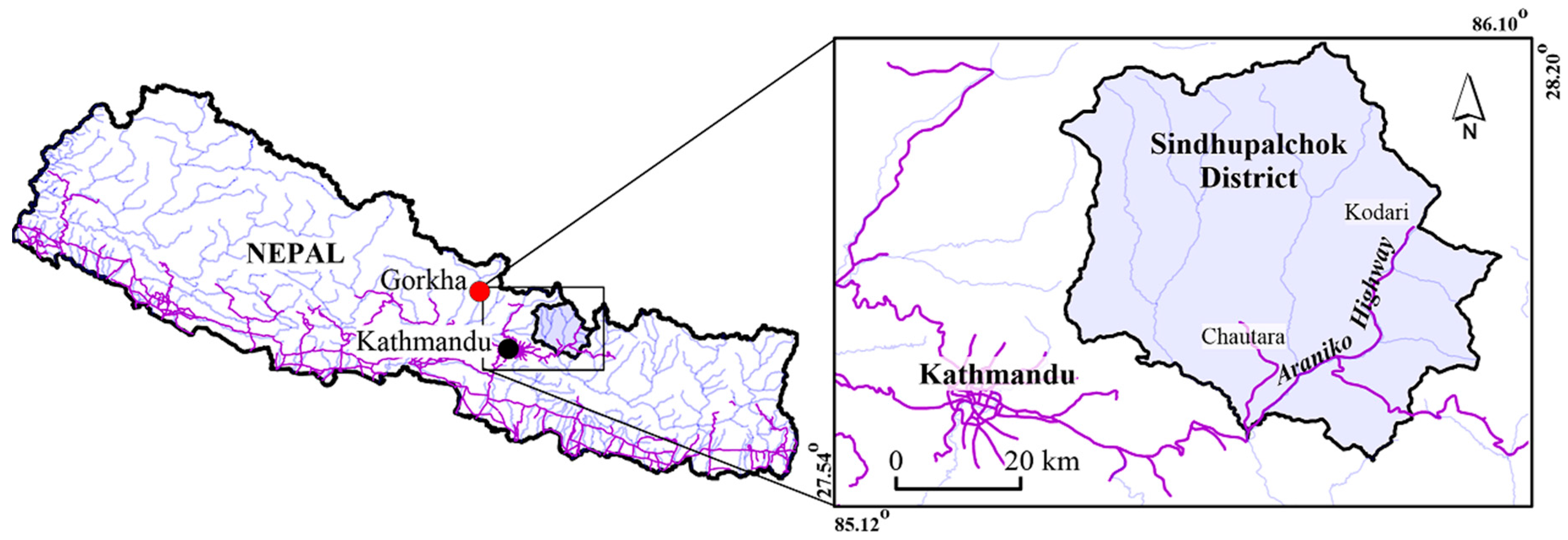
The Sindhupalchowk District study area, lies in the central part of Nepal (79.44° E–80.07° E, 27.61° N–28.2° N) at an elevation of 750–7080 m asl, covering an area of 2542 km2. As a result of the large elevation range, it has three different types of climates: tropical up to 1000 m asl, sub-tropical from 1000 to 2000 m asl, and temperate above 2000 m asl. Annual rainfall is approximately 2500 mm, and temperature varies from 7.5 °C to 32 °C. The area is mountainous and rich in natural resources, and the people depend entirely on agriculture for their survival. The district lies partly in the Mid-Hills and partly in the High-Hills, and exhibits very rugged terrain with deeply dissected gullies. Generally, the area has a predominantly gentle slope with cultivated land followed by forests in the upper part of the hills at steeper slope angles. It has a fragile topography with steep to moderate slopes, and the tectonic structures that initiate slope instability. In particular, the Arniko Highway, the only highway links Nepal to China (Figure 1), was heavily damaged and blocked by several landslides following the Gorkha earthquake.
Geologically, the study area lies between the Higher Himalaya and the Lesser Himalaya [38]. The Higher Himalayan Sequence covers about 65% of the study area, which consists of Precambrian (Higher Himalayan Crystalline rocks) high-grade metamorphic rocks such as gneisses, quartzite, schists, migmatite, and marble [39]. In some areas, Higher Himalayan gneisses have intruded into this sequence. Similarly, the Lesser Himalayan Sequence covers 35% of the study area and consists of Precambrian to Late Paleozoic rocks such as slate, dolomite, quartzite, augen gneiss, and limestone. The area of investigation is transgressed by the northerly inclined Main Central Thrust (MCT), which separates the Higher Himalayan Sequence and Lesser Himalayan Sequence tectonically.
3. Data Used
3.1. Landslide Inventory
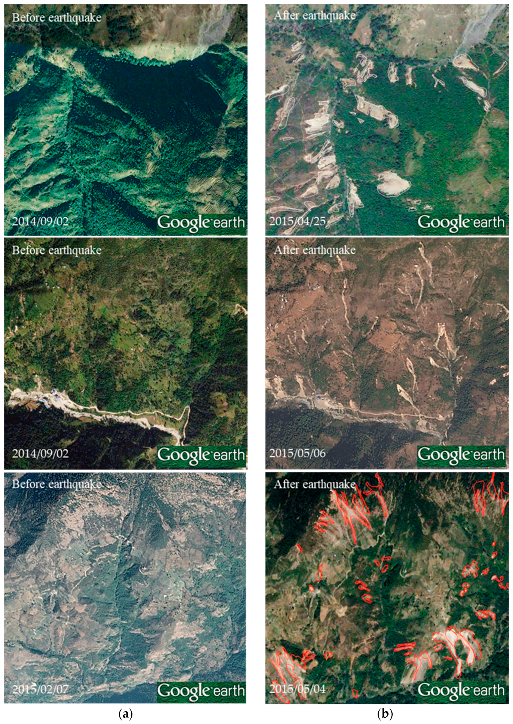
The precise delineation of landslide location is crucial for landslide susceptibility assessment of an area [40,41,42]. Thus, it is necessary to prepare an inventory map of co-seismic landslides. In this research, landslide locations were detected by compiling previous research and reports [2,3,43], and manual interpretation of Google Earth images. Google Earth provides a good alternative data source in inaccessible areas, and high-resolution imagery can be downloaded and combined with a geographical information system (GIS) [44]. Earthquake-induced landslides were located by comparing pre- and post-event imagery using historical timeline feature tools in Google Earth (Figure 2), and were then exported from Google Earth into the GIS environment.
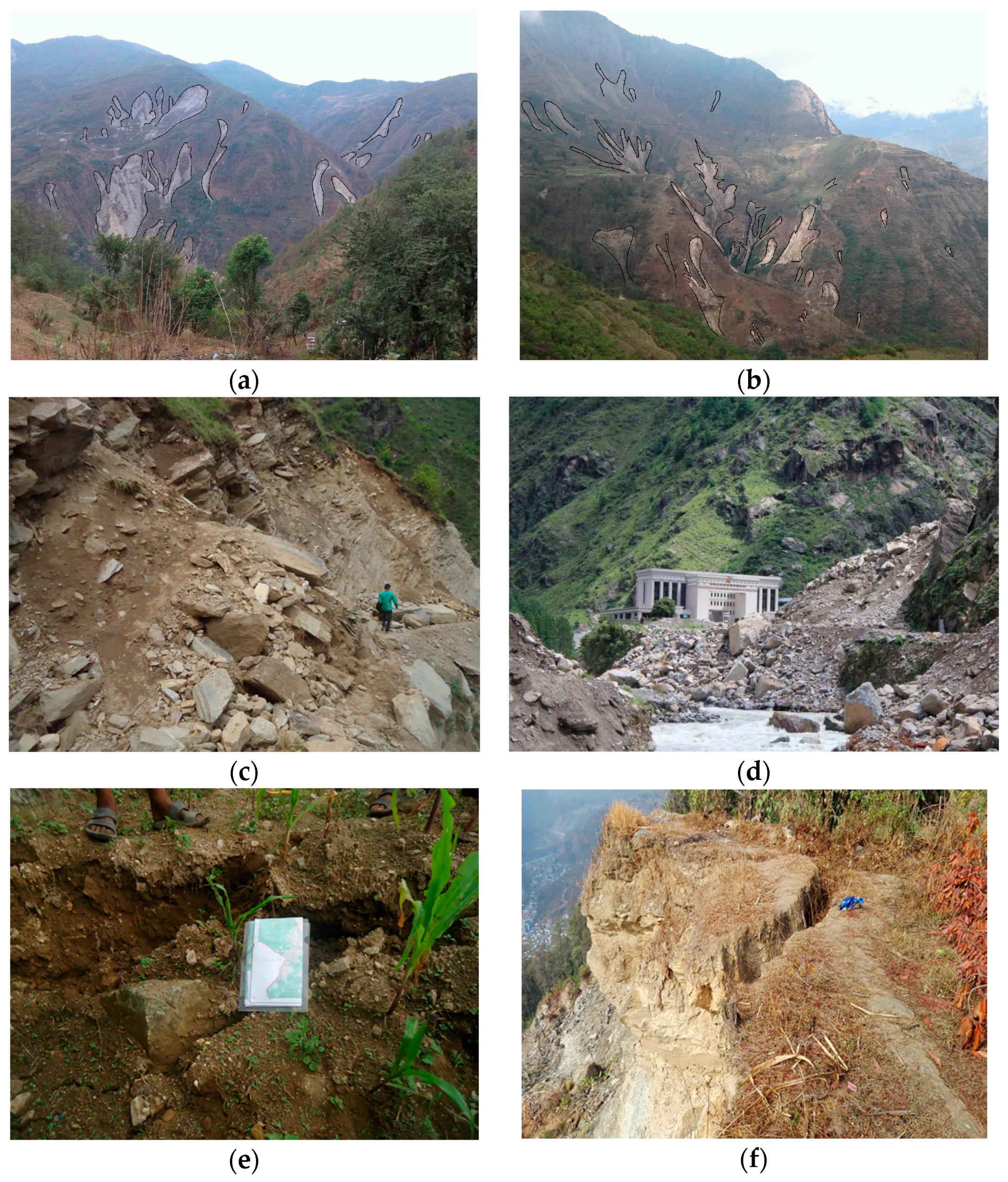
A field survey was conducted to correct existing landslide inventory maps in accessible parts of Sindhupalchowk District, thus increasing the reliability of the maps. In this survey, differences in landslide detectability and erosion were evaluated at 240 different locations (Figure 3). Local people were consulted about the presence and absence of landslides in their vicinity. Most of the observed landslides were rock falls and colluvium failures; however, all types of landslides were considered in combination in order to evaluate the probability associated with the earthquake event.
Through the image analysis and field survey, 2194 co-seismic landslides were identified covering area of 20.75 m2 to 95,029 m2 (average 3983 m2). In this study, a landslide initiation area was considered as a landslide point to prepare inventory data. Petschko et al. [45] employed a different landslide inventory sampling strategy, i.e., point inventory and polygon inventory, and they observed only small differences in the predictive capability of the model.
In this study, the data set of identified landslide was randomly split into two subsets: (i) the training data (1536 items; ~70%); and (ii) model validation data (658 items; ~30%), as shown in Figure 4. To ensemble with RF, the model needs landslide and non-landslide areas. Therefore, landslide initiation points were assigned a value of “1” and remaining pixels were assigned a value of 0.
3.2. Landslide Causative Factors
In this study, 11 causative factors (CFs) were collected from various sources and grouped into four types: seismic, geologic, topographic, and hydrologic as shown in Table 1. Several studies [2,3,4,5,43] have shown that these CFs are important in landslide analyses, and they are used to prepare landslide susceptibility maps, as shown in Table S1.
A digital elevation model (DEM) for the study area was generated from topographic maps at a scale of 1:25,000. The DEM resolution is 30 m × 30 m, and based on the DEM, all other CFs were rasterized for further analysis.
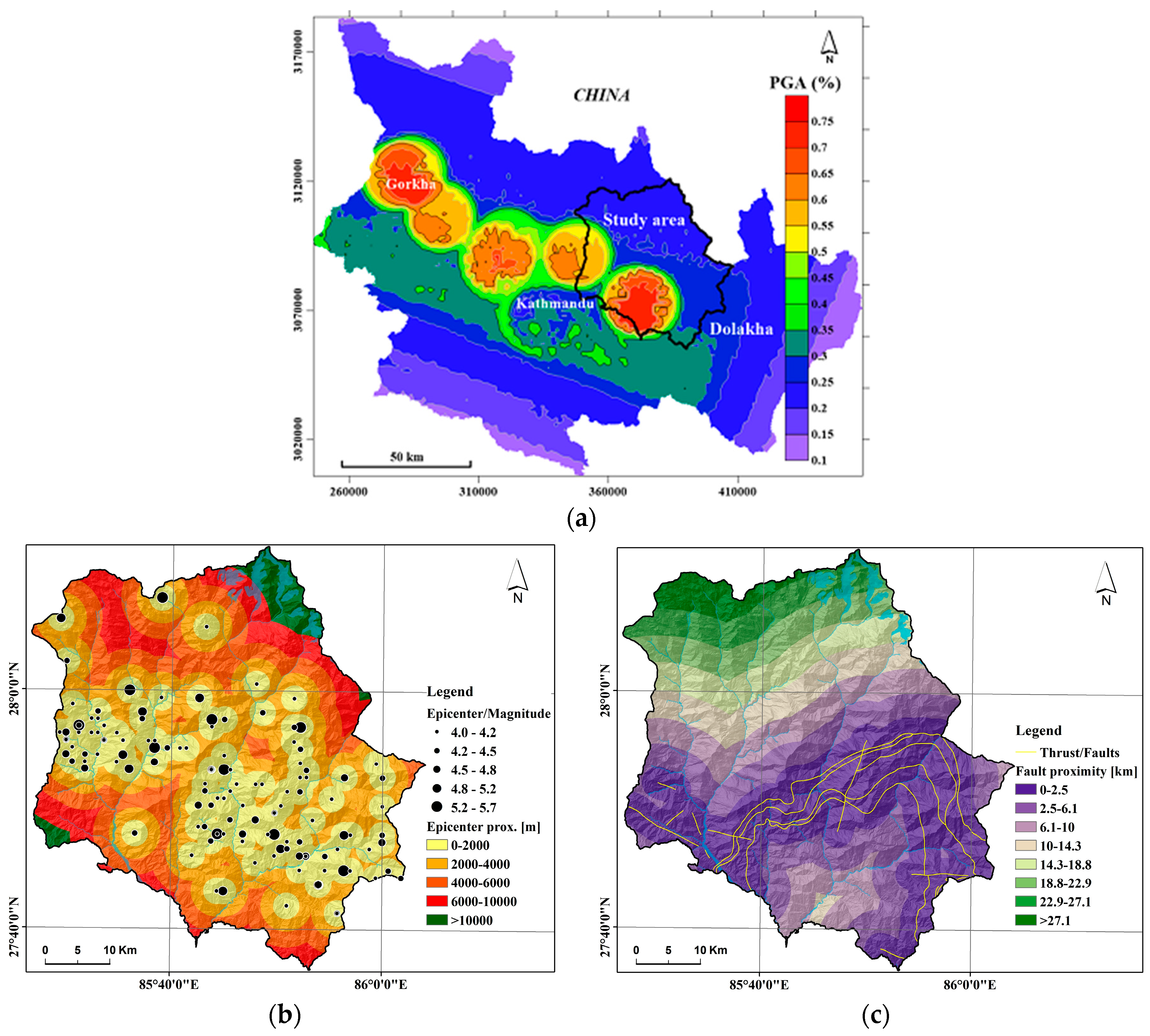
Peak ground acceleration (PGA), epicenter proximity, and seismic fault proximity were selected as seismic parameters for statistical analysis of the co-seismic landslides. Co-seismic landslides are triggered by strong ground-shaking acting on a rock mass. The strength of the ground-shaking can be calculated from the maximum acceleration, i.e., PGA, which is used to represent the seismic hazard scenario [46]. The PGA data of the Gorkha earthquake were obtained from the US Geological Survey (USGS 2015), and ranged from <0.24 to >0.68 g, as presented in Figure 5a. According to the USGS, the PGA map comprised eight classes: <0.24 g, 0.24–0.28 g, 0.28–0.36 g, 0.36–0.44 g, 0.44–0.52 g, 0.52–0.60 g, 0.60–0.68 g, and >0.68 g. In general, there is greater vibration near the epicenter, where many of the co-seismic landslides therefore occur. In this study, 133 epicenters were located using the locations of aftershocks >4 (Mb), published by the USGS (http://earthquake.usgs.gov). From these epicenters, an epicenter proximity map was prepared using the Euclidean distance function, comprising five classes: <2 km, 2–4 km, 4–6 km, 6–10 km, and >10 km, as shown in Figure 5b. A natural break method [47] was employed to classify the epicenter proximity. This is a data clustering method designed to determine the best arrangement of values in different classes [48]. The strength of rock mass decreases in the proximity of active faults, weakening the hillslope and leading to further instability [49]. A fault map was extracted from a geological map prepared by Dhital [39]. To determine the proximity of the faults, the Euclidean distance function was used and classified using the natural break scheme as: <2.5 km, 2.5–6.1 km, 6.1–10 km, 10–14.3 km, 14.3–18.8 km, 18.8–22.9 km, 22.9–27.1 km, and >27.1 km, as shown in Figure 5c.
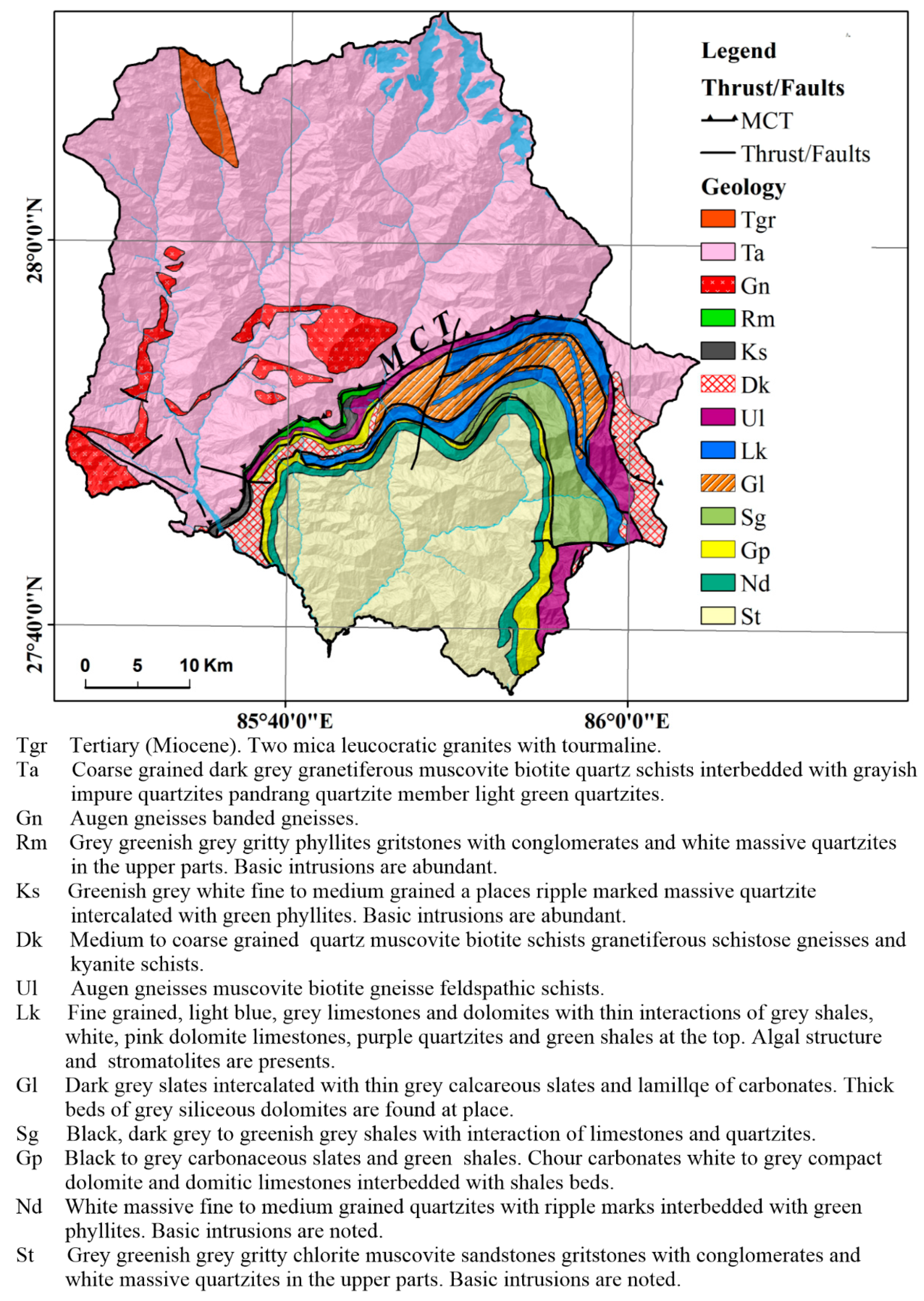
Geology strongly affects the distribution of landslides. It is widely recognized that geological parameters greatly influence the occurrence of landslides, because different lithological units have varying physical properties, leading to variations in the permeability and strength of rocks and soils [50]. In this study, the lithological layers were extracted by modifying geological maps of Nepal [39]. The data were divided into 13 lithological units, as depicted in Figure 6.
The spatial distribution of topographic attributes, including elevation, slope, curvature, and internal relief, was extracted using GIS. Although there is no direct relationship between elevation and landslide occurrence, research has shown an increase in landslide occurrence at higher elevation [51]. In Sindhupalchowk district, the elevation ranged from 750 m to 5013 m asl. The elevation was divided into 10 classes using the natural break algorithm in the GIS, i.e.,: <1281 m, 1281–1755 m, 1755–2254 m, 2254–3302 m, 3302–3850 m, 3850–4424 m, 4424–4973 m, 4973–5621 m, 5621–6968 m, and >6968 m asl (Figure 7a). The terrain slope calculates the gradient at any pixel on the surface which was derived from the first derivative function of the DEM. In this area, slope ranges from 0 to 71.2°. For analysis, the slope data were divided into five classes: <16°, 16–26.5°, 26.5–35.9°, 35.9–45.8°, and >45.8° using the natural break algorithm (Figure 7b). Another important CF is plan curvature, which measures the rate of change of terrain aspect angle measured in the horizontal plane. This can be used to differentiate between ridges and valleys. Plan curvature was calculated from a second-order derivative of the DEM. It was divided into concave, straight slope (plan slope), and convex, as shown in Figure 7c. Internal relief is defined as the elevation differences within a unit area, and was computed as the difference between the maximum and minimum altitudes per 900 m2. Internal relief shows the topographic breakage regarding slope and provides an indication of the potential energy available for mass wasting and soil erosion. Internal relief was divided into five classes: <47 m, 47–74 m, 74–104.7 m, 104.7–149.8 m, and >149.8 m (Figure 7d).
Drainage proximity, sediment transport index (STI). and topographic wetness index (TWI) are hydrological factors that play vital roles in slope instability [52]. During ground shaking, saturated or partially saturated soil slope lose strength and behave like a liquid. The Euclidean function in GIS was used to calculate eight drainage proximity classes throughout the study: <50 m, 50–100 m, 100–200 m, 200–400 m, 400–600 m, 600–800 m, 800–1000 m, and >1000 m (Figure 8a). By combining the length and steepness of slope, STI was calculated. It characterizes erosion and the deposition process [53]. STI was classified into five groups via the natural break classification method: <7.1, 7.1–12.3, 12.3–18.1, 18.1–28.2, and >28.2 (Figure 8b). Similarly, TWI is a steady-state wetness index that is commonly used to quantify topographic control on hydrological processes. The natural break method was also used to classify TWI into five groups: <5, 5–6.9, 6.9–9.4, 9.4–13.9, and >13.9 (Figure 8c).
4. Methodology
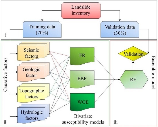
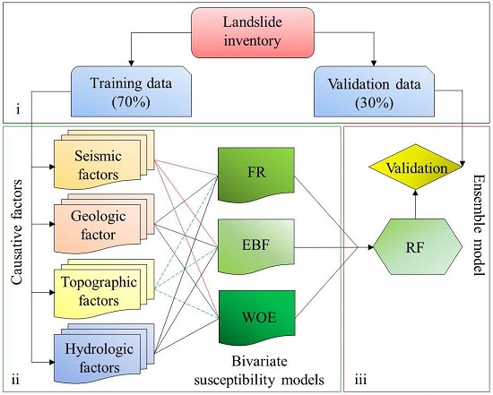
This study investigated the efficiency of bivariate statistical analysis and ensemble models for mapping landslide susceptibility. Figure 9 is an overview of the approach that was applied for the co-seismic landslide susceptibility mapping in the study area. The flow chart consists of three distinct phases: (i) collection of landslide inventory data, with collected data separated into training data and validation data; (ii) collection of landslide CFs and application of three popular bivariate statistical models (FR, EBF, and WOE) to analyze landslide susceptibility using a training data set; and (iii) combining the results from three bivariate models into an ensemble of the RF model, which was then validated using landslide validation data.
4.1. Frequency Ratio Method
The frequency ratio (FR) is the area where landslides occurred as the proportion of the total study area, and is also the ratio of the probabilities of a landslide occurrence versus non-occurrence for a given attribute [54]. First, the FR was calculated for each range of CF, and these FRs were then summed to calculate landslide susceptibility. FR can be defined as in Equation (1):
where, is the percentage of landslides in class i of parameter j, and is the percentage of a certain class of i of the parameter j. If the ratio is >1, then the relationship between the occurrence of landslides and the given CF is stronger, and vice versa [26].
4.2. Evidential Belief Function
The Dempster–Shafer theory of evidence was first proposed by Shafer [55], considered as a spatial integration model with mathematical representation. The estimation of EBFs from evidential data always relates to the proposition that the EBFs consist of four functions: degree of belief (Bel), uncertainty (Unc), disbelief (Dis), and plausibility (Pls). Bel and Pls interpret the lower and the upper degrees of belief that the evidence supports a proposition. This means that Bel and Pls are “pessimistic” and “optimistic” measures, respectively, of the spatial association of landslide occurrence with each class of evidence. The Bel represents the distribution of landslide occurrences [22,53,56]. Thus, only the Bel function was transformed into the landslide susceptibility map.
Suppose, a study area T consists of a total number of pixels N(T), landslide D occurs in a number of pixels N(D). The classes of CF in T are given by Cij (j = 1, 2, ..., m), then by overlaying a binary map (i.e., 0 = absence, 1 = presence) of D on each evidential map, the numbers of pixels Cij overlapping [i.e., N(Cij ∩ D)] and not overlapping [i.e., N(Cij) − N(Cij ∩ D)] with pixels containing D are calculated. Equation (2) shows the EBF (Bel) function:
where
The numerator to calculate parameter is the conditional probability of the existence of the landslide, while the denominator is a conditional probability where D exists in the absence of Cij.
4.3. Weight of Evidence
Spiegelhalter and Knill-Jones [57] introduced WOE in the medical field. Good [58] derived the WOE as a measure of the amount of information defined a piece of evidence. Bonham-Carter [59] introduced a mathematical formulation of the WOE method to produce mineral potential maps, based on the Bayesian probability framework [60,61]. In recent decades, the WOE method was introduced to landslide susceptibility modeling [19,22,25,62], and showed high reliability in investigating the spatial relationships and the distribution of special features [26,63]. Weights for each landslide CF, Cij are estimated based on the presence or absence of landslides D within the various classes of a given causative factor, as shown in Equations (3) and (4);
where W+ and W− are the weights of the presence or absence of landslides between a certain group of a CF. Equation (3) gives the conditional probability of occurrence of landslides and Equation (4) gives the same for the absence of landslides. Weight contract is the difference between the two weights , which gives the strength of correlation between the expected variable and landslides [64]. The weight contrast is positive/negative when there is a positive/negative association between the landslide and CFs class.
4.4. Ensemble with Random Forest
The general RF method was first proposed by Ho [65]. RF classification is basically a machine-learning algorithm developed by Breiman [66]. According to Williams [67], the RF algorithm tends to produce highly precise results, since the instability provided by the ensemble can be observed when creating a single decision tree. RF approaches have been used in the classification of remote sensing images [37,68], but seldom in landslide susceptibility studies [69,70]. In a single classification tree, small changes in the training data produce a large variance that usually points to low classification certainty. The basic idea of RFs is to expand multiple decision trees for a random subset of variables associated with training data.
RFs give various outputs for analyzing results that consist of out-of-bag (OOB) accuracy and evaluate the contribution of CF. As an alternative to cross-validation, RF classification provides OOB errors. In the case of the classification of formally non-identified data, RFs take advantage of the large variance between individual trees, where each tree votes for class membership and the respective class is allowed according to the majority of votes. These ensembles show robust and exact performance for complex data, with little requirement for fine-tuning in the presence of large, noisy variables. The RF method does not require assumptions, and can combine categorical and continuous parameters [71]. The present study makes extensive use of the “ModelMap” package [72], which is implemented in the R statistical programming environment [73].
5. Results
5.1. Landslide Inventory Distribution Analysis
The spatial distributions of landslides in each class of CF was analyzed using the spatial analysis tool in GIS. All landslides were considered in order to calculate the spatial relationship between CFs and landslide distribution.
The analysis results show that the number of landslides is less in areas where the PGA is high (Figure 10a). This finding is in contrast with the statement given in Section 3.2, where areas of high PGA show moderate slope distribution. Roback et al. [74] also showed that the landslide density from the Gorkha earthquake does not correlate directly with modeled PGA, where high-density landslides occur at relatively low values of modeled PGA (mostly 0.2–0.3 g). The overlap between PGA and landslide density (per square kilometer) is presented in Figure 10b. The correlation between landslides and epicenter proximity shows that the frequency of landslides decreases as distance from the epicenter increases (Figure 10c). Similarly, as shown in Figure 10d, considering fault proximity, co-seismic landslides were found to be strongly controlled by fault proximity.
The correlation analysis showed that the highest frequency distribution of landslides occurred in the Precambrian rock sequence (Ta), as shown in Figure 10e. This sequence mainly comprises highly jointed and fractured sedimentary and low-grade metamorphic rocks, such as slate, shale, siltstone, sandstone, quartzite, and garnetiferous and graphitic schist [39].
In terms of elevation, most of the landslides were confined to an elevation range of 1281 m to 3302 m asl (Figure 10f), as most of the aftershock epicenters were concentrated within this elevation range. In addition, most of the landslides were concentrated along slopes of 26.5° to 45.8° because the colluvium deposits rest on these slopes and became unstable during the shocks. Slopes steeper than 45.8° (Figure 10g) were found to have a low frequency of landslides as neither colluvium nor weathered soil can rest on such gradients [75]. In the case of plan curvature, the planner and convex slopes showed higher landslide frequencies than concave slopes (Figure 10h), because convex rounded hillslopes may be exposed to continuous swelling and contraction of loose debris on an inclined slope [50]. In general, higher internal relief exhibited high possibility of landslides [76]. In the study area, landslides are mainly concentrated on internal relief ranges from 47 m to 149.8 m (Figure 10i) because internal reliefs above 149.8 m consist of bare rocks without colluvial deposits.
Landslide frequency increases with proximity to drainage (Figure 10j). Rivers create steep slopes in their vicinities, and water can adversely affect the slope angle by cutting the toe of the terrain.
In case of STI, landslide frequency decreases with lower STI values. Areas with low STI values experience less erosion, whereas those with high values indicate the action of erosion on the topography. Higher landslide frequencies are distributed in areas with moderate STI values (7.1–18.1), as shown in Figure 10k. Landslide occurrence is more common in areas with low TWI values (Figure 10l). Higher TWI value represents a higher-order drainage channel, whereas low TWI value indicates lower-order drainage channels, which increase instability.
5.2. Landslide Susceptibility Mapping
Eleven CFs were used to prepare the landslide susceptibility maps. As described earlier (Section 3), only 70% of the total landslides (training data) were considered in the models.
5.2.1. Application of Bivariate Models
Correlation analysis was performed between landslides location and CFs. The spatial relationship between seismic CFs and landslides is shown in Table S2. The FR, EBF (Bel), and WOE weightings showing the probability of the occurrence of landslides, highly correlated with PGA values from 0.28 to 0.6. In terms of epicenter proximity, the probability of the occurrence of landslides existed at distances less than 2000 m. As the fault proximity increased, the probability of the occurrence of landslides decreased (Table S2).
The spatial relationships between geology and landslide are presented in Table S3. It shows that rock formation Sg has the highest probability, followed by Rm in the FR model. Similarly, in the EBF model, rock formation Sg has the highest probability, followed by Rm, Lk, Gl, and Nd. In the WOE model, landslide probability showed negative correlation with geological formations Tgr, Ta, and St.
Table S4 shows the spatial relationship between topographic CFs and the probability of landslide occurrence. Elevations of 1281–3302 m appeared to show a greater probability of landslide occurrence than other elevation ranges because most of the aftershocks were distributed in this range. The slope range of 35.9–45.8° was highly correlated with the occurrence of landslides. The WOE value showed that areas below 35.9 and above 45.8° were unfavorable for landslide occurrence. FR and EBF (Bel) values indicated that all slope shapes had reasonably similar probability values, whereas the WOE value showed a negative correlation with concave and planner slopes. Internal reliefs of 14.75–149.8 showed a correlation between FR and EBF (Bel) values for probable landslide occurrences. In the WOE model, internal reliefs of 74–149.8 had a good positive correlation with occurrence of landslides.
The spatial relationship between hydrologic CFs and landslides is given in Table S5. The proximity to drainage showed high FR and EBF (Bel) values. WOE values showed that proximities less than 50–200 m were positively correlated with the probability of landslides occurrence. High STI values reflected high erosion rates, and therefore indicated low stability. Low TWI values showed high FR and EBF (Bel) values, and WOE values with TWI < 5 were positively correlated with landslide occurrences.
After calculating the FR, EBF (Bel), and WOE weightages, all values were assigned to the corresponding classes of CFs and then overlaid to prepare three landslide susceptibility maps, respectively. By overlaying and calculating the landslide frequency, the FR weightage were calculated for all CFs. Then, FR values of the eleven landslide CFs were calculated using Equation (1). Figure 11a shows the results for the FR model; this mapping represents the integration of all of the weight maps on a cell-by-cell basis. Similarly, using the predicted values of EBF (Bel), the landslide susceptibility map of the study area was produced (Figure 11b). The weights of WOE were allocated to each CF group, and the resulting thematic maps were superposed and numerically summed to obtain a landslide susceptibility map using WOE (Figure 11c).
5.2.2. Application of the Ensemble Model
In the present study, an ensemble of RFs was applied for landslide susceptibility mapping of Sindhupalchowk District, Nepal. RF is commonly applied for data prognosis and analysis purposes. It has numerous attractive features such as the capacity to handle correlation and composite interactions of high dimensional data. The RF algorithm selects an arbitrary feature on each node of a split variable set [77], and tends to produce highly accurate models. To produce the ensemble, the three previously obtained susceptibility maps using FR, EBF (Bel), and WOE, 2000 trees and three variables for the separation point were considered at every node.
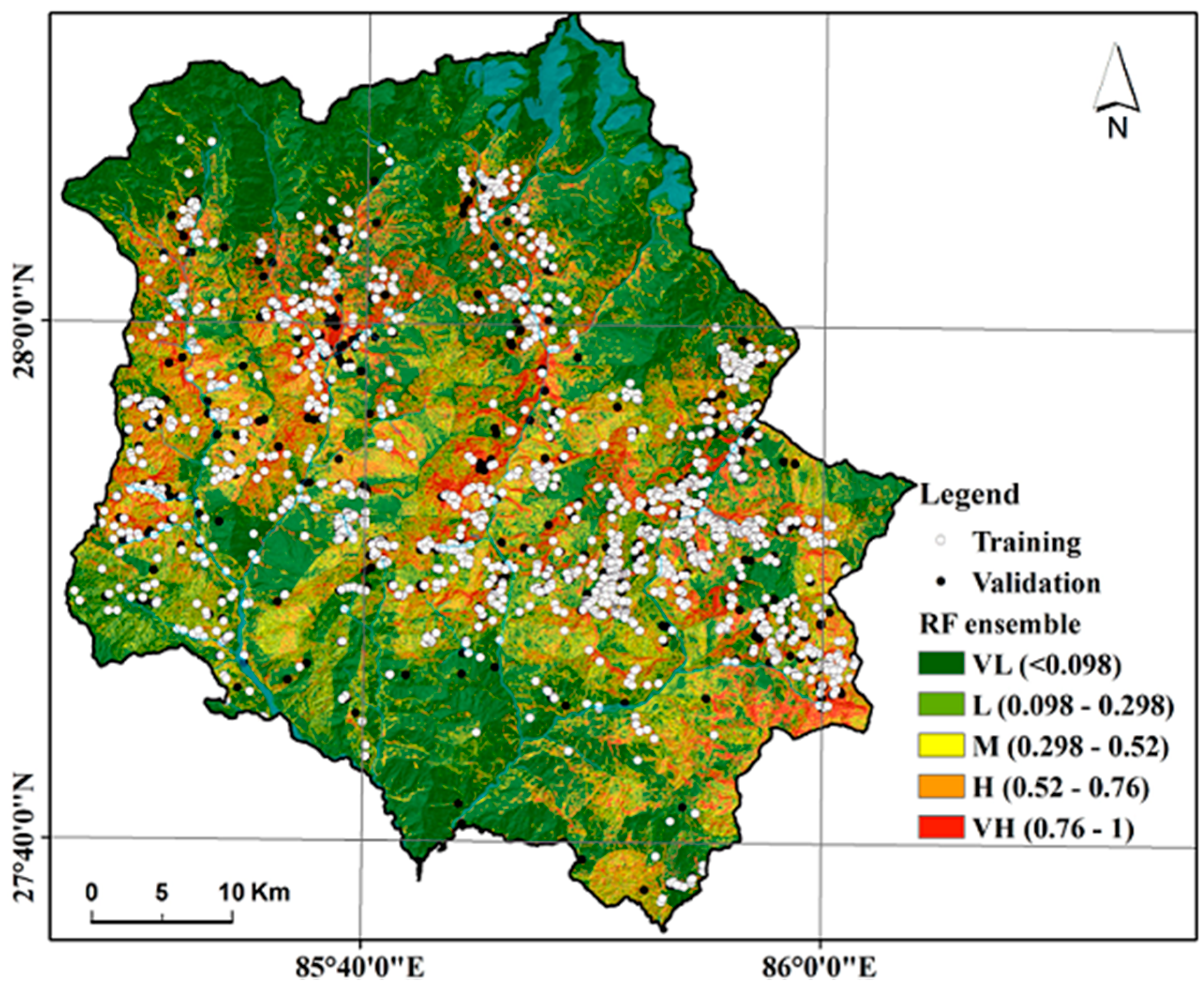
Finally, the ensemble RF was used to prepare the landslide susceptibility map, and the natural break classification scheme was used to classify the map into very low, low, moderate, high, and very high susceptibility classes in the GIS [19,56]. The map obtained from the ensemble RF method indicated that approximately 46.56% of the study area had very low susceptibility to landslides, and of the remainder 16.59%, 13.95%, 11.72%, and 11.16% were flagged as having low, moderate, high, and very high susceptibilities, respectively (Figure 12).
6. Validation of Ensemble Landslide Susceptibility Map
The receiver operating characteristic (ROC) curve was used to calculate the performance of a landslide susceptibility map prepared using the three bivariate models, and the RF ensemble model. In the ROC analysis, the area under the curve (AUC) characterized the nature of a forecast system [78]. The quantitative–qualitative relationship between prediction accuracy and AUC could be categorized as follows: 0.5–0.6, poor; >0.6–0.7, average; >0.7–0.8, good; >0.8–0.9, very good; and >0.9–1, excellent [79]. The success rates were retrieved by comparing the landslide training data with the results of FR, EBF (Bel) and WOE (Figure 13a). The figure shows that the EBF (Bel) had the highest AUC value (0.835), followed by the FR model (0.812) and WOE (0.801).
For validation of the RF model, training and validation data were used to determine the success rate and prediction rate of the given model. Lee [80] described the accuracy of the predictor variable; the model predicted landslides from the prediction rate curve. The success rate curve showed an AUC value of 0.91, while the prediction rate curve showed an AUC value of 0.969 (Figure 13b). From these results, the RF model was found to perform excellently in assessing susceptibility to co-seismic landslide.
7. Discussion
Landslides, like other natural hazards such as floods, earthquakes, and avalanches, are often difficult to predict [81]. A range of methods exist to assess the stability of slopes during earthquakes, including stress-deformation analyses and Newmark’s sliding-block model [82,83] that can be used directly in the design of engineering works as well as in the quantification of risk. Unfortunately, such methods are not suitable in the present scenario, because of the large number of events and the large spatial extent of the study area [84]. Fortunately, the development of GIS capabilities has provided a suitable platform for the analysis of large numbers of landslides covering large areas, and allows the incorporation of seismic shaking, geological, topographic and hydrologic parameters. However, there are no agreed, universal guidelines for selecting CFs [85,86] nor for selecting the number and size of CF classes. Therefore, the selection of landslide CFs and the number of classes were determined according to the geo-environmental characteristics of the study area, the mechanism of landslide occurrences, and other similar landslide prediction studies and available institutional resources [87]. Previous studies used a range of differing CFs to produce the landslide susceptibility maps. The prediction accuracy of a landslide model is highly dependent on the method used, and the same set of CFs can produce different accuracies with different methods. Therefore, the investigation of new methods is necessary to avoid such drawbacks [87]. In this study, 11 CFs were considered for modeling landslide susceptibility maps using three bivariate techniques: FR, EBF, and WOE, and the obtained results were combined using an ensemble RF model. The RF model, not sensitive to overfitting or to outliers in the training dataset [66].
A direct comparison of the present landslide susceptibility maps with those of previous studies is problematic, due to differences in sampling strategies, spatial scales, predictor sets, and model evaluation techniques. Consistent with the present findings, Pourghasemi and Kerle [88] also reported that a coupled approach employing the RF method with an EBF method in the western province of Iran found to be applicable and improved predictive accuracy. In the study by Umar et al. [89], the ensemble model applied in Sumatera, Indonesia showed reasonable efficiency for susceptibility mapping of the earthquake induced landslide. Xu et al. [90] applied a neural network approach to the spatial prediction of co-seismic landslides related to the 2008 earthquake in Wenchuan, China. In that case, such soft computing technologies did not achieve better results than traditional bivariate models and logistic regression models.
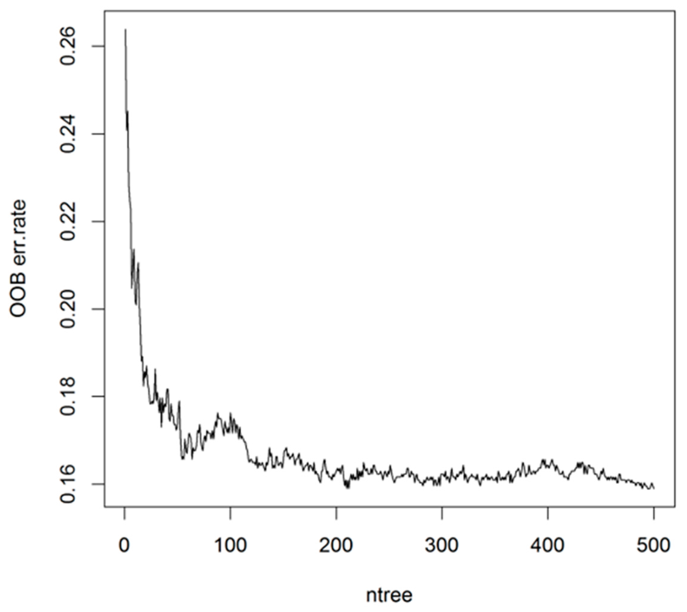
However, in the present study, the results showed that the RF ensemble model performed better than individual bivariate models for predicting co-seismic landslide susceptibility. To access the accuracy of this model, out-of-bag error (OOB) analysis was also carried out. The model was run as a function of increasing trees to identify the minimum number of trees required to minimize OOB errors. Figure 14 shows that the OOB error started stabilizing from 500 trees onwards. Thus, the optimal configuration of the model was considered to be 500 trees. Since an OOB error rate of 19.07% was obtained, the accuracy of the model is 80.93%, showing that the model is performs reasonably well [55].
In addition, it should be noted that the performances of the model can also be influenced by other items, such as the selection of CFs, and by the training and validation landslide data. Therefore, further attention should be paid on this issue in future studies.
8. Conclusions
On 25 April 2015, a large (MW 7.8) earthquake struck Nepal, triggering thousands of landslides in the central region of the Nepal Himalaya and resulting in the loss of more than 9000 lives. Bivariate models, including the FR, EBF, and WOE, were applied and compared using 11 CFs related to landslide susceptibility. A random forest (RF) ensemble was then applied to combine these models and generate a final landslide susceptibility map. From 2194 identified landslides, 1536 (~70%) were randomly selected to train the model and the remaining 658 (~30%) were used for model validation. The distributions of landslides in each CFs class were analyzed using GIS software. To ensemble the three susceptibility maps obtained using FR, EBF (Bel) and WOE, 2000 trees were selected, and for each node, only three variables were considered for the separation point. This achieved an OOB error of 19.07%, with the model showing a reasonable good accuracy of 80.93%. From this, it could be concluded that the model is reasonably good. Lastly, using the ensemble RF, a landslide susceptibility map was created and classified. The obtained map indicated that 46.56% of the study area shows low landslide susceptibility to landslides, whereas 16.59%, 13.95%, 11.72%, and 11.16% of the area have low, moderate, high, and very high susceptibilities, respectively. The ROC curve was employed to determine the performance of the landslide susceptibility map, and the AUC was determined to assess the quality of the forecast system. The EBF (Bel) model showed the highest AUC value (0.835), followed by the FR (0.812) and WOE (0.801) models. These values indicates that all the models achieve excellent accuracy. The RF model was validated using training and validation data to determine the success rate and prediction rate of the model. The success rate curve had an AUC value of 0.91, while the prediction rate curve had an AUC value of 0.969, indicating excellent performance for assessing co-seismic landslide susceptibility.
Supplementary Materials
The following are available online at www.mdpi.com/2220-9964/6/11/365/s1.
Acknowledgments
The authors are thankful to the anonymous reviewers for their valuable comments, which were very helpful in revising the manuscript to its present form. This work was supported by the National Research Foundation of Korea (NRF) grant funded by the Korean government (MSIT: Ministry of Science and ICT) (No. NRF–2017M2A8A4015042).
Author Contributions
Suchita Shrestha performed the research, analyzed the data, and wrote the paper. Tae-Seob Kang designed the research, the code tests, and extensively updated the paper. Madan Krishna Suwal was involved in data collection. All authors read and approved the final manuscript.
Conflicts of Interest
The authors declare no conflicts of interest.
References
- Ministry of Home Affairs. Ministry of Home Affairs (MoHA) and Disaster Preparedness Network–Nepal; Nepal Disaster Report 2015; Government of Nepal: Nepal, 2015; p. 180.
- Kargel, J.S.; Leonard, J.; Shugar, D.H.; Haritashya, U.K.; Bevington, A.; Fielding, E.J.; Fujita, K.; Geertsema, M.; Miles, E.S.; Steiner, J.; et al. Geomorphic and geologic controls of geohazards induced by Nepal’s 2015 Gorkha earthquake. Science 2016, 351, aac8353. [Google Scholar] [CrossRef] [PubMed]
- Regmi, A.D.; Dhital, M.R.; Zhang, J.Q.; Su, L.J.; Chen, X.Q. Landslide susceptibility assessment of the region affected by the 25 April 2015 Gorkha earthquake of Nepal. J. Mt. Sci. 2016, 13, 1941–1957. [Google Scholar] [CrossRef]
- Kritikos, T.; Robinson, T.R.; Davies, T.R. Regional coseismic landslide hazard assessment without historical landslide inventories: A new approach. J. Geophys. Res. Earth Surf. 2015, 120, 711–729. [Google Scholar] [CrossRef] [Green Version]
- Xu, C.; Xu, X.; Yao, X.; Dai, F. Three (nearly) complete inventories of landslides triggered by the May 12, 2008 Wenchuan Mw 7.9 earthquake of China and their spatial distribution statistical analysis. Landslides 2014, 11, 441–461. [Google Scholar] [CrossRef]
- Papadopoulos, G.A.; Plessa, A. Magnitude-distance relations for earthquake-induced landslides in Greece. Eng. Geol. 2000, 58, 377–386. [Google Scholar] [CrossRef]
- Jibson, R.W.; Harp, E.L.; Michael, J.A. A method for producing digital probabilistic seismic landslide hazard maps. Eng. Geol. 2000, 58, 271–289. [Google Scholar] [CrossRef]
- Lee, C.T.; Huang, C.C.; Lee, J.F.; Pan, K.L.; Lin, M.L.; Dong, J.J. Statistical approach to earthquake–induced landslide susceptibility. Eng. Geol. 2008, 100, 43–58. [Google Scholar] [CrossRef]
- Gorum, T.; Fan, X.; van Westen, C.J.; Huang, R.Q.; Xu, Q.; Tang, C.; Wang, G. Distribution pattern of earthquake–induced landslides triggered by the 12 May 2008 Wenchuan earthquake. Geomorphology 2011, 133, 152–167. [Google Scholar] [CrossRef]
- Miles, S.B.; Keefer, D.K. Comprehensive areal model of earthquake–induced landslides: Technical specification and user guide. US. Geol. Survey 2007. [Google Scholar]
- Miles, S.B.; Keefer, D.K. Evaluation of CAMEL—Comprehensive areal model of earthquake–induced landslides. Eng. Geol. 2009, 104, 1–15. [Google Scholar] [CrossRef]
- Anbalagan, R. Landslide hazard evaluation and zonation mapping in mountainous terrain. Eng. Geol. 1992, 32, 269–277. [Google Scholar] [CrossRef]
- Pachauri, A.K.; Pant, M. Landslide hazard mapping based on geological attributes. Eng. Geol. 1992, 32, 81–100. [Google Scholar] [CrossRef]
- Mehrotra, G.S.; Sarkar, S.; Kanungo, D.P.; Mahadevaiah, K. Terrain analysis and spatial assessment of landslide hazards in parts of Sikkim Himalaya. J. Geol. Soc. India 1996, 47, 491–498. [Google Scholar]
- Sarkar, S.; Kanungo, D.P.; Mehrotra, G.S. Landslide hazard zonation: A case study in Garhwal Himalaya, India. Mt. Res. Dev. 1995, 15, 301–309. [Google Scholar] [CrossRef]
- Chen, G.; Meng, X.; Tan, L.; Zhang, F.; Qiao, L. Comparison and combination of different models for optimal landslide susceptibility zonation, Quarterly. J. Eng. Geol. Hydrogeol. 2014, 47, 283–306. [Google Scholar] [CrossRef]
- Molteni, F.; Buizza, R.; Palmer, T.N.; Petroliagis, T. The ECMWF ensemble prediction system: Methodology and validation. Q. J. R. Meteorol. Soc. 1996, 122, 73–119. [Google Scholar] [CrossRef]
- Marsigli, C.; Montani, A.; Nerozzi, F.; Paccagnella, T.; Tibaldi, S.; Molteni, F.; Buizza, R. A strategy for high-resolution ensemble prediction. II: Limited-area experiments in four Alpine flood events. Q. J. R. Meteorol. Soc. 2001, 127, 2095–2115. [Google Scholar] [CrossRef]
- Mohammady, M.; Pourghasemi, H.R.; Pradhan, B. Landslide susceptibility mapping at Golestan Province, Iran: A comparison between frequency ratio, Dempster–Shafer, and weights–of–evidence models. J. Asian Earth Sci. 2012, 61, 221–236. [Google Scholar] [CrossRef]
- Regmi, A.D.; Devkota, K.C.; Yoshida, K.; Pradhan, B.; Pourghasemi, H.R.; Kumamoto, T.; Akgun, A. Application of frequency ratio, statistical index, and weights–of–evidence models and their comparison in landslide susceptibility mapping in Central Nepal Himalaya. Arab. J. Geosci. 2014, 7, 725–742. [Google Scholar] [CrossRef]
- Jaafari, A.; Najafi, A.; Pourghasemi, H.R.; Rezaeian, J.; Sattarian, A. GIS–based frequency ratio and index of entropy models for landslide susceptibility assessment in the Caspian forest, northern Iran. Int. J. Environ. Sci. Technol. 2014, 11, 909–926. [Google Scholar] [CrossRef]
- Ding, Q.; Chen, W.; Hong, H. Application of frequency ratio, weights of evidence and evidential belief function models in landslide susceptibility mapping. Geocarto Int. 2017, 32, 619–639. [Google Scholar] [CrossRef]
- Althuwaynee, O.F.; Pradhan, B.; Lee, S. Application of an evidential belief function model in landslide susceptibility mapping. Comput. Geosci. 2012, 44, 120–135. [Google Scholar] [CrossRef]
- Lee, S.; Hwang, J.; Park, I. Application of data–driven evidential belief functions to landslide susceptibility mapping in Jinbu, Korea. Catena 2013, 100, 15–30. [Google Scholar] [CrossRef]
- Hong, H.; Ilia, I.; Tsangaratos, P.; Chen, W.; Xu, C. A hybrid fuzzy weight of evidence method in landslide susceptibility analysis on the Wuyuan area, China. Geomorphology 2017, 290, 1–16. [Google Scholar] [CrossRef]
- Poli, S.; Sterlacchini, S. Landslide representation strategies in susceptibility studies using weights–of–evidence modeling technique. Nat. Resour. Res. 2007, 16, 121–134. [Google Scholar] [CrossRef]
- Kayastha, P.; Dhital, M.R.; De Smedt, F. Landslide susceptibility mapping using the weight of evidence method in the Tinau watershed, Nepal. Nat. Hazards 2012, 63, 479–498. [Google Scholar] [CrossRef]
- Tsangaratos, P.; Ilia, I.; Hong, H.; Chen, W.; Xu, C. Applying Information Theory and GIS-based quantitative methods to produce landslide susceptibility maps in Nancheng County, China. Landslides 2017, 14, 1091–1111. [Google Scholar] [CrossRef]
- Thiery, Y.; Malet, J.P.; Sterlacchini, S.; Puissant, A.; Maquaire, O. Landslide susceptibility assessment by bivariate methods at large scales: Application to a complex mountainous environment. Geomorphology 2007, 92, 38–59. [Google Scholar] [CrossRef] [Green Version]
- Neuhäuser, B.; Terhorst, B. Landslide susceptibility assessment using “weights-of-evidence” applied to a study area at the Jurassic escarpment (SW-Germany). Geomorphology 2007, 86, 12–24. [Google Scholar] [CrossRef]
- Pham, B.T.; Bui, D.T.; Dholakia, M.B.; Prakash, I.; Pham, H.V.; Mehmood, K.; Le, H.Q. A novel ensemble classifier of rotation forest and Naïve Bayer for landslide susceptibility assessment at the Luc Yen district, Yen Bai Province (Viet Nam) using GIS. Geomat. Nat. Hazards Risk 2016, 1–23. [Google Scholar] [CrossRef]
- Hong, H.; Pourghasemi, H.R.; Pourtaghi, Z.S. Landslide susceptibility assessment in Lianhua County (China): A comparison between a random forest data mining technique and bivariate and multivariate statistical models. Geomorphology 2016, 259, 105–118. [Google Scholar] [CrossRef]
- Youssef, A.M.; Pourghasemi, H.R.; Pourtaghi, Z.S.; Al–Katheeri, M.M. Landslide susceptibility mapping using random forest, boosted regression tree, classification and regression tree, and general linear models and comparison of their performance at Wadi Tayyah Basin, Asir Region, Saudi Arabia. Landslides 2016, 13, 839–856. [Google Scholar] [CrossRef]
- Dou, J.; Oguchi, T.; Hayakawa, Y.S.; Uchiyama, S.; Saito, H.; Paudel, U. GIS–Based Landslide Susceptibility Mapping Using a Certainty Factor Model and Its Validation in the Chuetsu Area, Central Japan; Landslide Science for a Safer Geoenvironment; Sassa, K., Canuti, P., Yin, Y., Eds.; Springer: Cham, Switzerland, 2014; pp. 419–424. [Google Scholar]
- Pourghasemi, H.R.; Rossi, M. Landslide susceptibility modeling in a landslide prone area in Mazandarn Province, north of Iran: A comparison between GLM, GAM, MARS, and M–AHP methods. Theor. Appl. Climatol. 2016. [Google Scholar] [CrossRef]
- Chen, W.; Panahi, M.; Pourghasemi, H.R. Performance evaluation of GIS–based new ensemble data mining techniques of adaptive neuro–fuzzy inference system (ANFIS) with genetic algorithm (GA), differential evolution (DE), and particle swarm optimization (PSO) for landslide spatial modelling. CATENA 2017, 157, 310–324. [Google Scholar] [CrossRef]
- Ham, J.; Chen, Y.; Crawford, M.M.; Ghosh, J. Investigation of the random forest framework for classification of hyperspectral data. IEEE Trans. Geosci. Remote Sens. 2005, 43, 492–501. [Google Scholar] [CrossRef]
- Sharma, C.K. Geology of Nepal Himalaya and Adjacent Countries; Sangeeta Sharma: Kathmandu, Nepal, 1990. [Google Scholar]
- Dhital, M.R. Geology of the Nepal Himalaya: Regional Perspective of the Classic Collided Orogen; Springer: Cham, Switzerland, 2015. [Google Scholar]
- Guzzetti, F.; Mondini, A.C.; Cardinali, M.; Fiorucci, F.; Santangelo, M.; Chang, K.T. Landslide inventory maps: New tools for an old problem. Earth Sci. Rev. 2012, 112, 42–66. [Google Scholar] [CrossRef]
- Harp, E.L.; Jibson, R.W. Landslides triggered by the 1994 Northridge, California, earthquake. Bull. Seismol. Soc. Am. 1996, 86, S319–S332. [Google Scholar]
- Keefer, D.K. Landslides caused by earthquakes. Geol. Soc. Am. Bull. 1984, 95, 406–421. [Google Scholar] [CrossRef]
- Tiwari, B.; Ajmera, B.; Dhital, S. Characteristics of moderate–to large–scale landslides triggered by the Mw 7.8 2015 Gorkha earthquake and its aftershocks. Landslides 2017, 1–22. [Google Scholar] [CrossRef]
- Corominas, J.; Van Westen, C.; Frattini, P.; Cascini, L.; Malet, J.P.; Fotopoulou, S.; Catani, F.; van Den Eeckhaut, M.; Mavrouli, O.; Agliardi, F.; et al. Recommendations for the quantitative analysis of landslide risk. Bull. Eng. Geol. Environ. 2014, 73, 209–263. [Google Scholar] [CrossRef] [Green Version]
- Petschko, H.; Bell, R.; Leopold, P.; Heiss, G.; Glade, T. Landslide Inventories for Reliable Susceptibility Maps in Lower Austria. In Landslide Science and Practice; Springer: Berlin/Heidelberg, Germany, 2013; pp. 281–286. [Google Scholar]
- Tsapanos, T.M. Appraisal of seismic hazard parameters for the seismic regions of the east circum–Pacific belt inferred from a Bayesian approach. Nat. Hazards 2003, 30, 59–78. [Google Scholar] [CrossRef]
- Mahalingam, R.; Olsen, M.J.; O’Banion, M.S. Evaluation of landslide susceptibility mapping techniques using lidar–derived conditioning factors (Oregon case study). Geomat. Nat. Hazard Risk 2016, 7, 1884–1907. [Google Scholar] [CrossRef]
- Jenks, G. The data model concept in statistical mapping. Int. Yearb. Cartogr. 1967, 7, 347–356. [Google Scholar]
- Dramis, F.; Sorriso–Valvo, M. Deep–seated gravitational slope deformations, related landslides and tectonics. Eng. Geol. 1994, 38, 231–243. [Google Scholar] [CrossRef]
- Pradhan, B.; Lee, S. Landslide susceptibility assessment and factor effect analysis: Backpropagation artificial neural networks and their comparison with frequency ratio and bivariate logistic regression modelling. Environ. Model. Softw. 2010, 25, 747–759. [Google Scholar] [CrossRef]
- Ercanoglu, M.; Gokceoglu, C. Use of fuzzy relations to produce landslide susceptibility map of a landslide prone area (West Black Sea Region, Turkey). Eng. Geol. 2004, 75, 229–250. [Google Scholar] [CrossRef]
- Gökceoglu, C.; Aksoy, H. Landslide susceptibility mapping of the slopes in the residual soils of the Mengen region (Turkey) by deterministic stability analyses and image processing techniques. Eng. Geol. 1996, 44, 147–161. [Google Scholar] [CrossRef]
- Pradhan, A.M.S.; Kang, H.S.; Lee, S.; Kim, Y.T. Spatial model integration for shallow landslide susceptibility and its runout using a GIS–based approach in Yongin, Korea. Geocarto Intern. 2016, 1–22. [Google Scholar] [CrossRef]
- Bonham-Carter, G.F. Geographic Information Systems for geoscientists–modeling with GIS. Comput. Methods Geosci. 1994, 13, 398. [Google Scholar]
- Shafer, G. A Mathematical Theory of Evidence; Princeton University Press: Princeton, NJ, USA, 1976; Volume 1, p. xiii–297. [Google Scholar]
- Pradhan, A.M.S.; Kim, Y.T. Spatial data analysis and application of evidential belief functions to shallow landslide susceptibility mapping at Mt. Umyeon, Seoul, Korea. Bull. Eng. Geol. Environ. 2016, 76, 1263–1279. [Google Scholar] [CrossRef]
- Spiegelhalter, D.J.; Knill-Jones, R.P. Statistical and knowledge–based approaches to clinical decision–support systems, with an application in gastroenterology. J. R. Stat. Soc. Ser. A 1984, 147, 35–77. [Google Scholar] [CrossRef]
- Good, I.J. Weight of Evidence: A Brief Survey. In Bayesian Statistics 2; Bernardo, J.M., DeGroot, M.H., Lindley, D.V., Smith, A.F.M., Eds.; Elsevier: New York, NY, USA, 1985; pp. 249–269. [Google Scholar]
- Bonham-Carter, G.F. Geographic Information Systems for Geoscientist: Modelling with GIS. In Computer Methods in the Geosciences; Merriam, D.F., Ed.; Pergamon/Elsevier: New York, NY, USA, 2002; Volume 13, pp. 302–334. [Google Scholar]
- Bonham-Carter, G.F.; Agterberg, F.P.; Wright, D.F. Integration of geological datasets for gold exploration in Nova Scotia. Digit. Geol. Geogr. Inf. Syst. 1988, 15–23. [Google Scholar] [CrossRef]
- Van Westen, C.J. The modelling of landslide hazards using GIS. Surv. Geophys. 2000, 21, 241–255. [Google Scholar] [CrossRef]
- Ilia, I.; Tsangaratos, P. Applying weight of evidence method and sensitivity analysis to produce a landslide susceptibility map. Landslides 2016, 13, 379–397. [Google Scholar] [CrossRef]
- Regmi, N.R.; Giardino, J.R.; Vitek, J.D. Modeling susceptibility to landslides using the weight of evidence approach: Western Colorado, USA. Geomorphology 2010, 115, 172–187. [Google Scholar] [CrossRef]
- Armaş, I. Weights of evidence method for landslide susceptibility mapping, Prahova Subcarpathians, Romania. Nat. Hazards 2012, 60, 937–950. [Google Scholar] [CrossRef]
- Ho, T.K. Random decision forests. In Proceedings of the Third international Conference on Document Analysis and Recognition, Montreal, QC, Canada, 14–15 August 1995. [Google Scholar]
- Breiman, L. Random forests. Mach. Learn. 2001, 5, 5–32. [Google Scholar] [CrossRef]
- Williams, G. Data Mining with Rattle and R: The Art of Excavating Data for Knowledge Discovery (Use R!); Springer Science+Business Media, LLC: New York, NY, USA, 2011. [Google Scholar] [CrossRef]
- Pal, M. Random forest classifier for remote sensing classification. Int. J. Remote Sens. 2005, 26, 217–222. [Google Scholar] [CrossRef]
- Vorpahl, P.; Elsenbeer, H.; Märker, M.; Schröder, B. How can statistical models help to determine driving factors of landslides? Ecol. Model. 2012, 239, 27–39. [Google Scholar] [CrossRef]
- Brenning, A. Spatial prediction models for landslide hazards: Review, comparison and evaluation. Nat. Hazards Earth Syst. Sci. 2005, 5, 853–862. [Google Scholar] [CrossRef]
- Catani, F.; Lagomarsino, D.; Segoni, S.; Tofani, V. Landslide susceptibility estimation by random forests technique: sensitivity and scaling issues. Nat. Hazards Earth Syst. Sci. 2013, 13, 2815–2831. [Google Scholar] [CrossRef]
- Freeman, E.; Frescino, T.; Freeman, M.E. Package ‘ModelMap’ 2016. Available online: ftp://mandriva.c3sl.ufpr.br/CRAN/web/packages/ModelMap/ModelMap.pdf (accessed on 5 July 2017).
- Venables, W.N.; Smith, D.M.; The R Development Core Team. An Introduction to R, Notes on R: A Programming Environment for Data Analysis and Graphics. Available online: https://cran.r-project.org/doc/manuals/R-intro.pdf (accessed on 5 July 2017).
- Roback, K.; Clark, M.K.; West, A.J.; Zekkos, D.; Li, G.; Gallen, S.F.; Chamlagain, D.; Godt, J.W. The size, distribution, and mobility of landslides caused by the 2015 M w 7.8 Gorkha earthquake, Nepal. Geomorphology 2017. [Google Scholar] [CrossRef]
- Magliulo, P.; Di, L.A.; Russo, F.; Zelano, A. Geomorphology and landslide susceptibility assessment using GIS and bivariate statistics: A case study in southern Italy. Nat. Hazards 2008, 7, 411–435. [Google Scholar] [CrossRef]
- Pradhan, A.M.S.; Kim, Y.T. Relative effect method of landslide susceptibility zonation in weathered granite soil: A case study in Deokjeok–ri Creek, South Korea. Nat. Hazards 2014, 72, 1189–1217. [Google Scholar] [CrossRef]
- Meyer, D.; Leisch, F.; Hornik, K. The support vector machine under test. Neurocomputing 2003, 55, 169–186. [Google Scholar] [CrossRef]
- Nandi, A.; Shakoor, A. A GIS–based landslide susceptibility evaluation using bivariate and multivariate statistical analyses. Eng. Geol. 2010, 110, 11–20. [Google Scholar] [CrossRef]
- Yesilnacar, E.K. The Application of Computational Intelligence to Landslide Susceptibility Mapping in Turkey. Ph.D. Thesis, University of Melbourne, Parkville, Australia, 2005. [Google Scholar]
- Lee, S. Application and verification of fuzzy algebraic operators to landslide susceptibility mapping. Environ. Geol. 2007, 52, 615–623. [Google Scholar] [CrossRef]
- Bui, D.T.; Tuan, T.A.; Klempe, H.; Pradhan, B.; Revhaug, I. Spatial prediction models for shallow landslide hazards: A comparative assessment of the efficacy of support vector machines, artificial neural networks, kernel logistic regression, and logistic model tree. Landslides 2016, 13, 361–378. [Google Scholar]
- Newmark, N.M. Effects of earthquakes on dams and embankments. Geotechnique 1965, 15, 139–160. [Google Scholar] [CrossRef]
- Miles, S.B.; Ho, C.L. Rigorous landslide hazard zonation using Newmark’s method and stochastic ground motion simulation. Soil Dyn. Earthq. Eng. 1999, 18, 305–323. [Google Scholar] [CrossRef]
- Van Western, C.J. Geo-information Tools for Landslide Risk Assessment: An Overview of Recent Developments. In Proceeding of the Ninth International Symposium on Landslides, Rio de Janeiro, Brazil, 28 June–2 July 2004; Landslides: Evaluation and Stabilization; Mauricio Ehrlich, W.L., Fontoura, S.A.B., Sayao, A.S.F., Eds.; Balkema, Taylor & Francis Group: London, UK, 2004; Volume 1, pp. 39–56. [Google Scholar]
- Xu, C.; Xu, X.; Yao, Q.; Wang, Y. GIS-based bivariate statistical modelling for earthquake-triggered landslides susceptibility mapping related to the 2008 Wenchuan earthquake, China. Q. J. Eng. Geol. Hydrogeol. 2013, 46, 221–236. [Google Scholar] [CrossRef]
- Ayalew, L.; Yamagishi, H. The application of GIS-based logistic regression for landslide susceptibility mapping in the Kakuda-Yahiko Mountains, Central Japan. Geomorphology 2005, 65, 15–31. [Google Scholar] [CrossRef]
- Chen, W.; Xie, X.; Wang, J.; Pradhan, B.; Hong, H.; Bui, D.T.; Duan, Z.; Ma, J. A comparative study of logistic model tree, random forest, and classification and regression tree models for spatial prediction of landslide susceptibility. Catena 2017, 151, 147–160. [Google Scholar] [CrossRef]
- Pourghasemi, H.R.; Kerle, N. Random forests and evidential belief function-based landslide susceptibility assessment in Western Mazandaran Province, Iran. Environ. Earth Sci. 2016, 75, 185. [Google Scholar] [CrossRef]
- Umar, Z.; Pradhan, B.; Ahmad, A.; Jebur, M.N.; Tehrany, M.S. Earthquake induced landslide susceptibility mapping using an integrated ensemble frequency ratio and logistic regression models in West Sumatera Province, Indonesia. Catena 2014, 118, 124–135. [Google Scholar] [CrossRef]
- Xu, C.; Xu, X.; Dai, F.; Saraf, A.K. Comparison of different models for susceptibility mapping of earthquake triggered landslides related with the 2008 Wenchuan earthquake in China. Comput. Geosci. 2012, 46, 317–329. [Google Scholar] [CrossRef]
Figure 1.
Map showing the location of Sindhupalchowk District.

Figure 2.
Google Earth images of landslides triggered by the earthquake: (a) before; (b) after the event.
Figure 2.
Google Earth images of landslides triggered by the earthquake: (a) before; (b) after the event.

Figure 3.
Co-seismic landslides observed during field survey: (a,b) landslides initiated on steep slopes; (c) rock topple; (d) rockslide partially damming the Bhote Koshi at Rasuwagadhi; (e) observed cracking; (f) hanging block.
Figure 3.
Co-seismic landslides observed during field survey: (a,b) landslides initiated on steep slopes; (c) rock topple; (d) rockslide partially damming the Bhote Koshi at Rasuwagadhi; (e) observed cracking; (f) hanging block.

Figure 4.
Landslide inventory map.
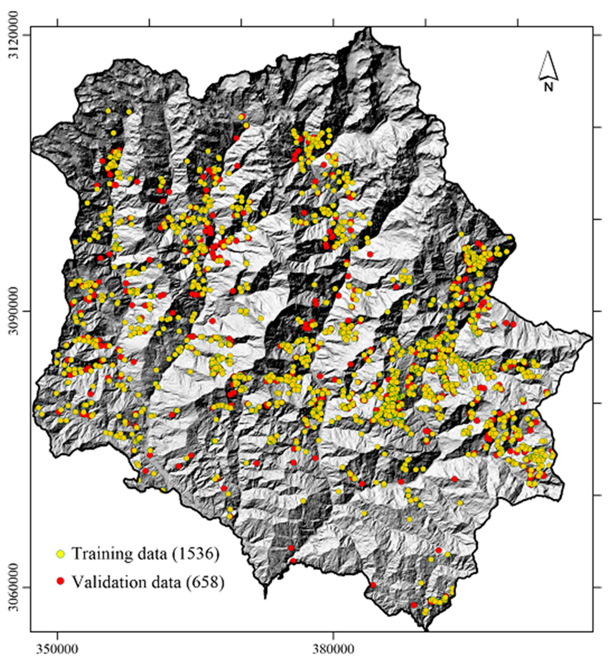
Figure 5.
Seismic causative factors: (a) peak ground acceleration (PGA) map of earthquake-affected areas; (b) epicenter proximity; (c) fault proximity.
Figure 5.
Seismic causative factors: (a) peak ground acceleration (PGA) map of earthquake-affected areas; (b) epicenter proximity; (c) fault proximity.

Figure 6.
Geological map of the study area (Modified from Dhital 2015).

Figure 7.
Topographic factors: (a) elevation; (b) slope; (c) plan curvature; (d) internal relief.
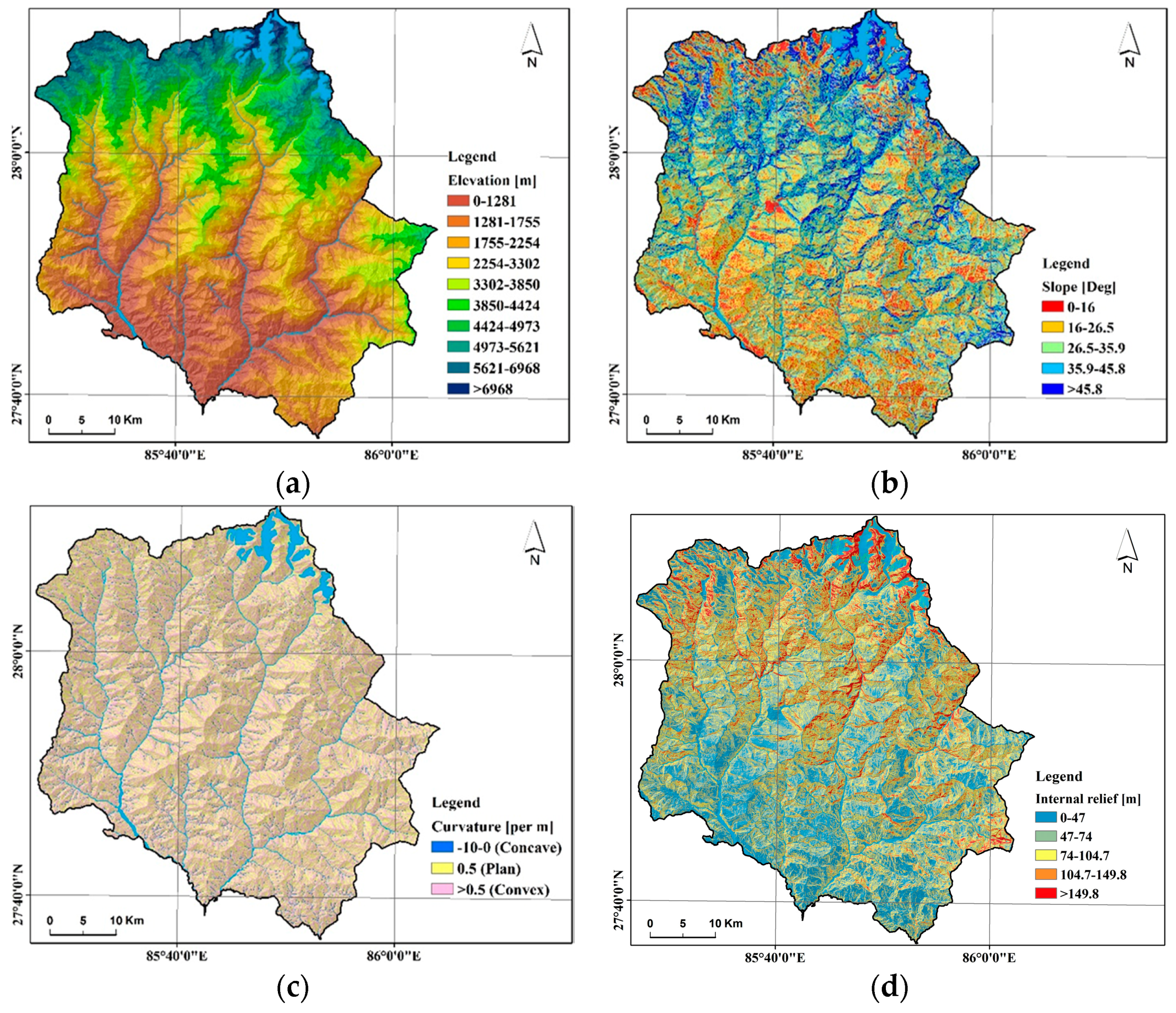
Figure 8.
Hydrologic factors: (a) drainage proximity; (b) sediment transport index (STI); (c) topographic wetness index (TWI).
Figure 8.
Hydrologic factors: (a) drainage proximity; (b) sediment transport index (STI); (c) topographic wetness index (TWI).
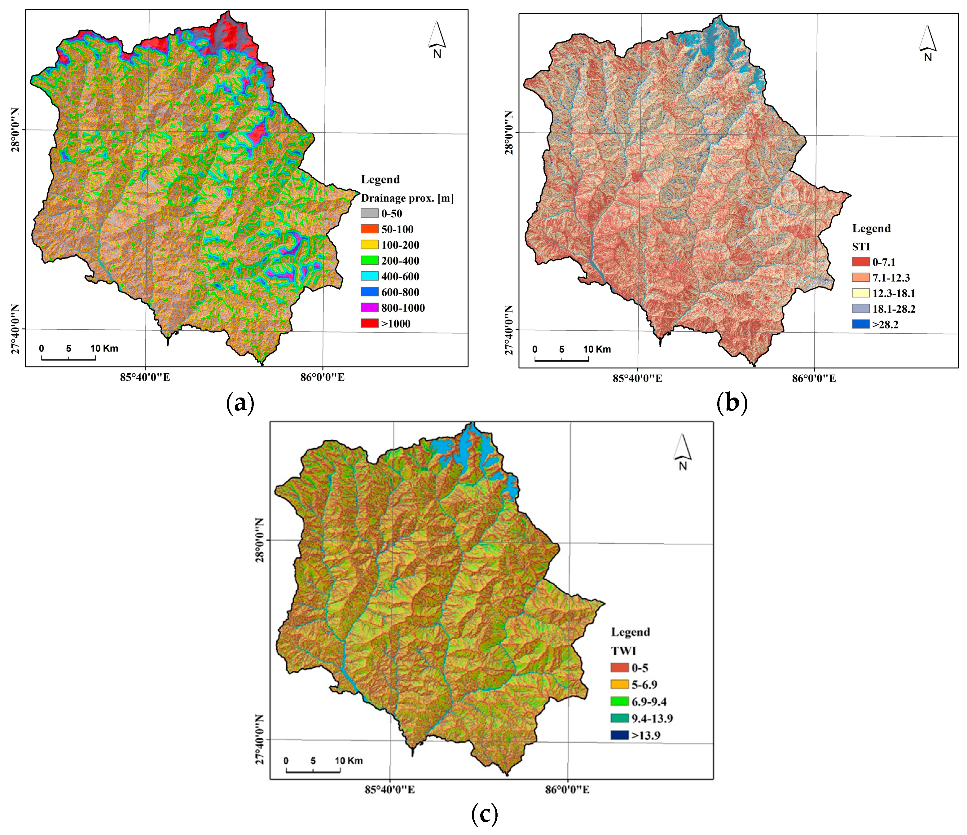
Figure 9.
Flow chart of the co-seismic landslide susceptibility modeling.
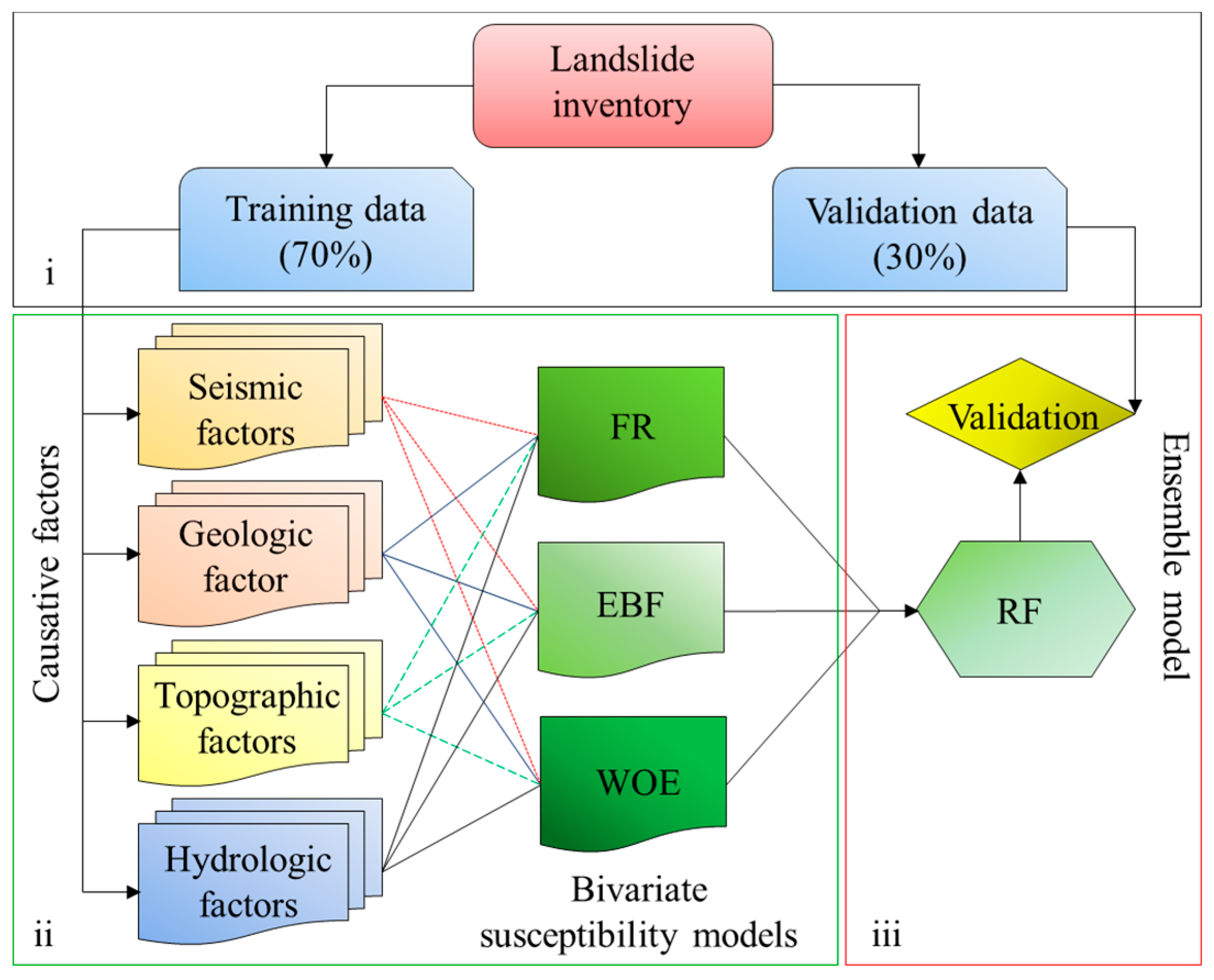
Figure 10.
Frequency of landslides and area of their influence: (a) PGA; (b) overlay between PGA and landslide density; (c) epicenter proximity; (d) fault proximity; (e) geology; (f) elevation; (g) slope; (h) plan curvature; (i) internal relief; (j) drainage proximity; (k) STI; (l) TWI.
Figure 10.
Frequency of landslides and area of their influence: (a) PGA; (b) overlay between PGA and landslide density; (c) epicenter proximity; (d) fault proximity; (e) geology; (f) elevation; (g) slope; (h) plan curvature; (i) internal relief; (j) drainage proximity; (k) STI; (l) TWI.
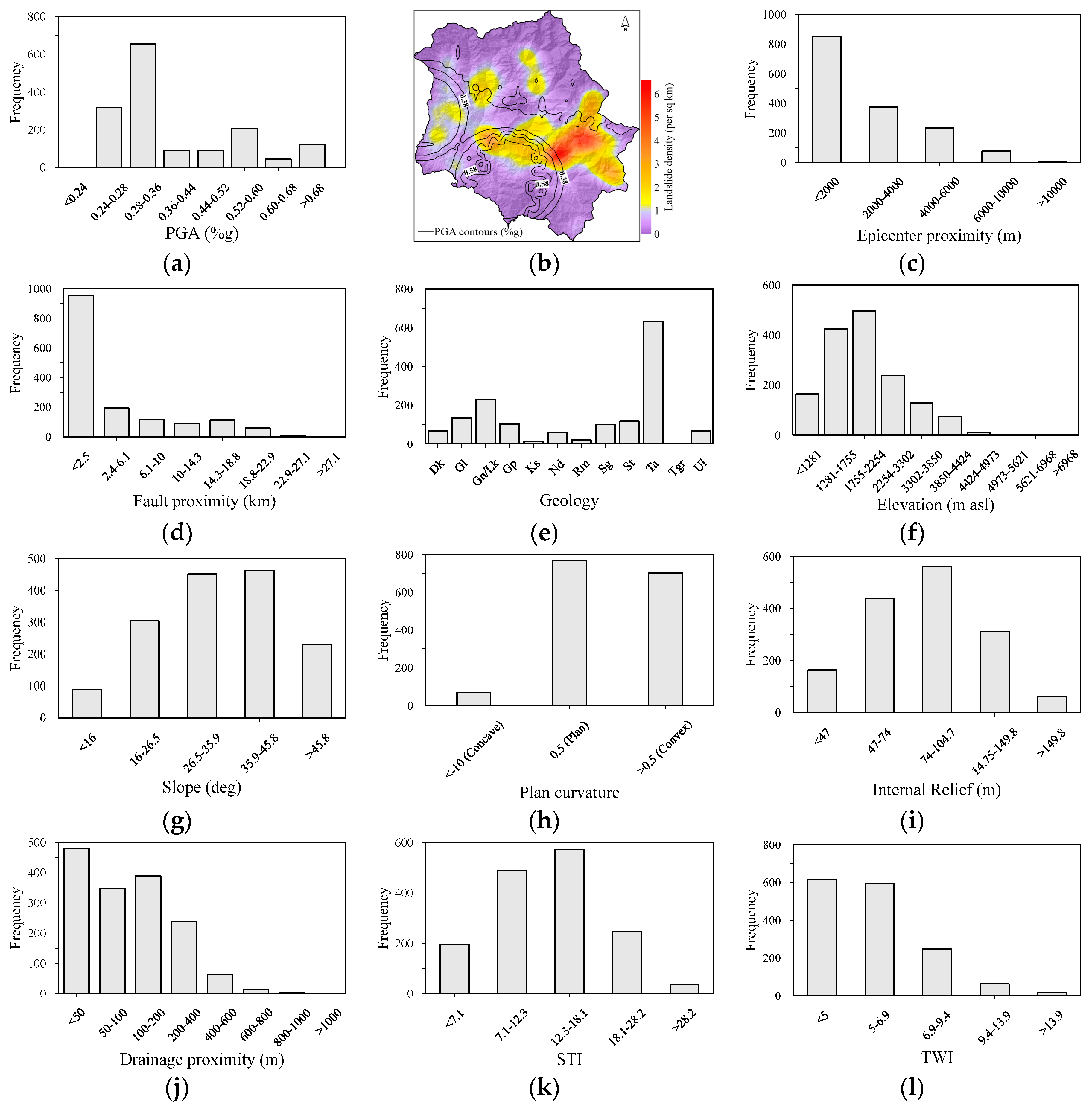
Figure 11.
Landslide susceptibility index: (a) FR model; (b) evidential belief function (EBF) (Bel) model; (c) weight of evidence (WOE) model.
Figure 11.
Landslide susceptibility index: (a) FR model; (b) evidential belief function (EBF) (Bel) model; (c) weight of evidence (WOE) model.
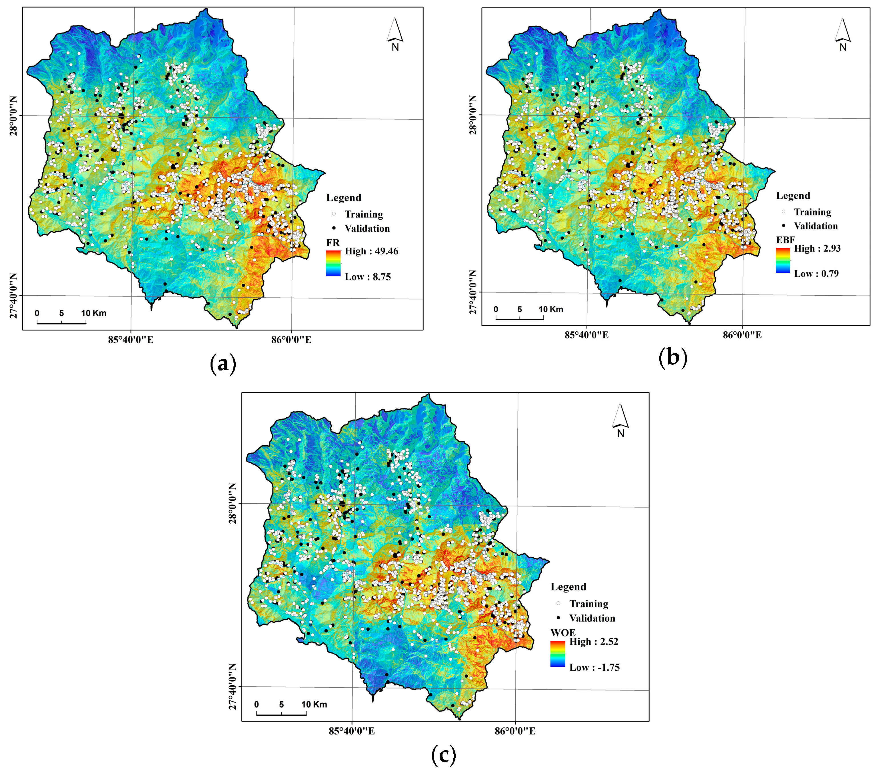
Figure 12.
Landslide susceptibility mapping using an ensemble of FR, EBF and WOE using the RF model.
Figure 12.
Landslide susceptibility mapping using an ensemble of FR, EBF and WOE using the RF model.

Figure 13.
Validation using a receiver operating characteristic curve (ROC). (a) Success rate curves of bivariate models (FR, EBF and WOE) using training data; (b) success rate and prediction rate of the ensemble RF landslide susceptibility model.
Figure 13.
Validation using a receiver operating characteristic curve (ROC). (a) Success rate curves of bivariate models (FR, EBF and WOE) using training data; (b) success rate and prediction rate of the ensemble RF landslide susceptibility model.

Figure 14.
Out-of-bag error plot of the random forest (RF) algorithm for the study area.

Table 1.
Data type, source and scale.
| Type | Causative Factor | Source/Producer | Scale |
|---|---|---|---|
| Seismic | Peak ground acceleration | USGS 2015/Rasterized in geographical information system (GIS) | 1:25,000 |
| Epileft proximity | Dhital (2015)/Euclidean analysis in GIS | 1:50,000 | |
| Fault proximity | Dhital (2015)/Euclidean analysis in GIS | 30 × 30 | |
| Geologic | Geology | Dhital (2015)/Rasterized in GIS | 1:50,000 |
| Topographic | Elevation | Department of Survey, Government of Nepal/Contour interval 20 m/DEM in GIS | 1:25,000 |
| Slope | GIS | 1:25,000 | |
| Plan curvature | GIS | 1:25,000 | |
| Internal relief | GIS | 1:25,000 | |
| Hydrologic | Drainage proximity | Department of Survey, Government of Nepal/Euclidean analysis in GIS | 1:25,000 |
| Sediment transport index | GIS | 1:25,000 | |
| Topographic wetness index | GIS | 1:25,000 |
© 2017 by the authors. Licensee MDPI, Basel, Switzerland. This article is an open access article distributed under the terms and conditions of the Creative Commons Attribution (CC BY) license (http://creativecommons.org/licenses/by/4.0/).
Share and Cite
MDPI and ACS Style
Shrestha, S.; Kang, T.-S.; Suwal, M.K. An Ensemble Model for Co-Seismic Landslide Susceptibility Using GIS and Random Forest Method. ISPRS Int. J. Geo-Inf. 2017, 6, 365. https://doi.org/10.3390/ijgi6110365
AMA Style
Shrestha S, Kang T-S, Suwal MK. An Ensemble Model for Co-Seismic Landslide Susceptibility Using GIS and Random Forest Method. ISPRS International Journal of Geo-Information. 2017; 6(11):365. https://doi.org/10.3390/ijgi6110365
Chicago/Turabian StyleShrestha, Suchita, Tae-Seob Kang, and Madan Krishna Suwal. 2017. "An Ensemble Model for Co-Seismic Landslide Susceptibility Using GIS and Random Forest Method" ISPRS International Journal of Geo-Information 6, no. 11: 365. https://doi.org/10.3390/ijgi6110365
Note that from the first issue of 2016, this journal uses article numbers instead of page numbers. See further details here.