Mapping and Analyzing Stream Network Changes in Watonwan River Watershed, Minnesota, USA

Abstract

Much of the Watonwan River tributary system to the upper Mississippi River basin (UMR), and the fluvial systems to which it drains, are listed as impaired under the United States Environmental Protection Agency Clean Water Act303(d) and/or by the Minnesota Pollution Control Agency. In addition, eutrophic conditions and excessive sedimentation rates exist in Lake Pepin, a riverine lake to which the UMR drains. Thus, understanding the hydrogeomorphic change throughout the UMR is vital in order to establish appropriate efforts to mitigate environmental hazards downstream. This study attempts to evaluate hydrogeomorphic change at the watershed scale in the Watonwan River watershed between 1855 and the near present. Historical plat maps, digital elevation models (DEMs), aerial images, soil/topographic characteristics, land-use change, and field surveys are analyzed. Surficial hydrologic features digitized from historical plat maps are compared with contemporary stream networks extracted from high-resolution DEMs. Scale effects are investigated using multi-resolution (1 m, 3 m, 8.5 m, and 30 m) DEMs, with 8.5 m DEMs being ideal for watershed scale analysis, and 1–3 m DEMs being ideal for subwatershed analysis. There has been a substantial hydrogeomorphic change in the watershed since 1855, but most significantly, we interpret that the highest rates of erosion occur in the eastern watershed, where knickzone propagation has produced substantial relief.

1. Introduction

Although sediment transport and erosion by streams are a natural part of the fluvial system, excessively high sediment loads can lead to the impairment of a stream [1], and can often lead to biodiversity loss and other associated environmental issues [2]. Significant reaches of the upper Mississippi River Basin (UMR) in the United States (US), are considered impaired for turbidity due to excess suspended sediment loading under section 303(d) of the United States Environmental Protection Agency (EPA) Clean Water Act. This accompanies ongoing environmental problems associated with turbidity, eutrophic conditions, and high sedimentation rates in Lake Pepin, a riverine lake at the mouth of the UMR (Figure 1; [1,2,3]).

The Minnesota River basin (MRB) is a tributary to the UMR, and supplies 80–90% of the suspended sediment load of the UMR, as measured from sediment cores from Lake Pepin (Figure 1; [2,3,4]). The background geomorphic history of the MRB has resulted in a landscape underlain primarily by glacial till and glaciofluvial sands that are now exposed to erosion by ongoing fluvial response to abrupt, postglacial base-level fall (~13.4 ka; e.g., [5,6]). The UMR is, therefore, naturally primed to produce large volumes of sediment throughout the Holocene. However, sedimentation rates have increased by an order of magnitude from pre-settlement to present [2,3]. The increase in sedimentation has led to an impairment listing and the loss of biodiversity, thus necessitating an investigation of the cause and nature of historic geomorphic and hydrologic change within the MRB. Prior research suggests that this increase is the result of more erosive rivers associated with significant land-cover/land-use change from native wetland and prairie to row crop agriculture, as well as the alteration of natural hydrologic pathways both on the surface and in the subsurface [7,8]. It may also be associated with higher discharges in this region related to ongoing climatic change [8,9]). In a recent study, Belmont et al. [1] identified fluvial processes eroding bluffs, banks, channel incision, and ravines as prominent point sources of sediment loading in the Le Sueur River, a tributary to the Minnesota River in the Greater Blue Earth River basin.

The Watonwan River, like the Le Sueur, is a tributary to the Blue Earth River (Figure 1), the largest tributary of the Minnesota River. The Watonwan River is located in south–central Minnesota, with a total area of 227,280 ha (561,620 acres) covered by six counties: Watonwan, Blue Earth, Cottonwood, Martin, Brown, and Jackson. The 182 km Watonwan River starts in central Cottonwood County and flows into the Blue Earth River approximately 13 km southwest of Mankato, Minnesota, US. The Greater Blue Earth River basin, including the Watonwan River and the Le Sueur River watersheds, contributes 55% of the suspended sediment load and 69% of the nitrate load to the Minnesota River at Mankato [10,11]. Due to a highly erodible substrate (primarily near surface lake sediments and underlying fine-grained glacial till and glaciofluvial sands) and higher, flashier flows attributed to climate, hydrologic, and land-use changes in the Watonwan River system, there has been a dramatic increase in erosion and, in turn, sediment loading in the watershed since European settlement in the late 1800s [12,13]. Clearly, these watersheds are undergoing significant changes, but that change is not yet fully or holistically understood. Restoration of water quality in the watershed requires accurate identification of the sediment supply [14] and an understanding of the changed landscape. The Watonwan’s proximity and similarity to intensively studied rivers such as the Le Sueur River [1,5] makes it an ideal case study watershed to further investigate historic geomorphic and hydrologic change at a watershed scale.

It is to the authors’ knowledge that no previous research has attempted to map watershed-scale stream network and surface hydrology change since European settlement in the middle 1800s in this area, particularly by using our oldest spatial record—the 1855 plat maps. Many have intensively investigated the geochemical signatures of sediment in transport [1,13,15], main-stem channel planform dynamics [16,17], and the long-term landscape evolution of main-stem drainage [5] in nearby streams to aid in understanding the environmental issues plaguing these watersheds. However, in this context, this study demonstrates a first attempt at evaluating geomorphic and hydrologic changes at a watershed scale in the Watonwan River watershed from 1855 to the present. According to the Minnesota Pollution Control Office (MPCA) [13], degraded water quality and biological communities were found throughout the Watonwan River watershed. For example, none of the 53 assessment units in the watershed passed for aquatic life general use. Tolerant fish species (e.g., white sucker and creek chub), which are known to exist in streams that are chemically impaired, habitat limited, sediment laden and/or high in nitrates, accounted for 74% of the total number of fish collected [13]. In addition to the persisting sediment problem, bacteria impairments were common throughout the watershed [13].

In this study, the watershed scale refers to the “Department of Natural Resources (DNR) Major Watershed” published in 2009, which is similar to the level 8 hydrological unit (HUC8 drainage unit) defined by the United States Geological Survey (USGS) [18]. Here, we use morphometric analysis and environmental data compilation to predict locations in the modern Watonwan watershed landscape that may be susceptible to erosional processes responsible for excess sediment loading. Therefore, the objectives of this research include: (1) mapping stream network change using digital 1855 General Land Office (GLO) plat maps and contemporary digital elevation models (DEMs); (2) analyzing scale effects using multi-source and multi-resolution (1 m, 3 m, 8.5 m, and 30 m) DEMs in the generation of flow networks; (3) evaluating major land-use and land-cover changes within changed areas of the stream network; (4) identifying those areas of highest potential for erosive point sources in the modern watershed informed by Belmont et al. [1]. The results from this research are an initial effort to aid researchers, landowners, and policy makers in understanding historical hydrogeomorphic and land use-change, as well as to predict, at the watershed scale, the locations of ongoing hydrogeomorphic change in the stream network.

2. Materials and Methods

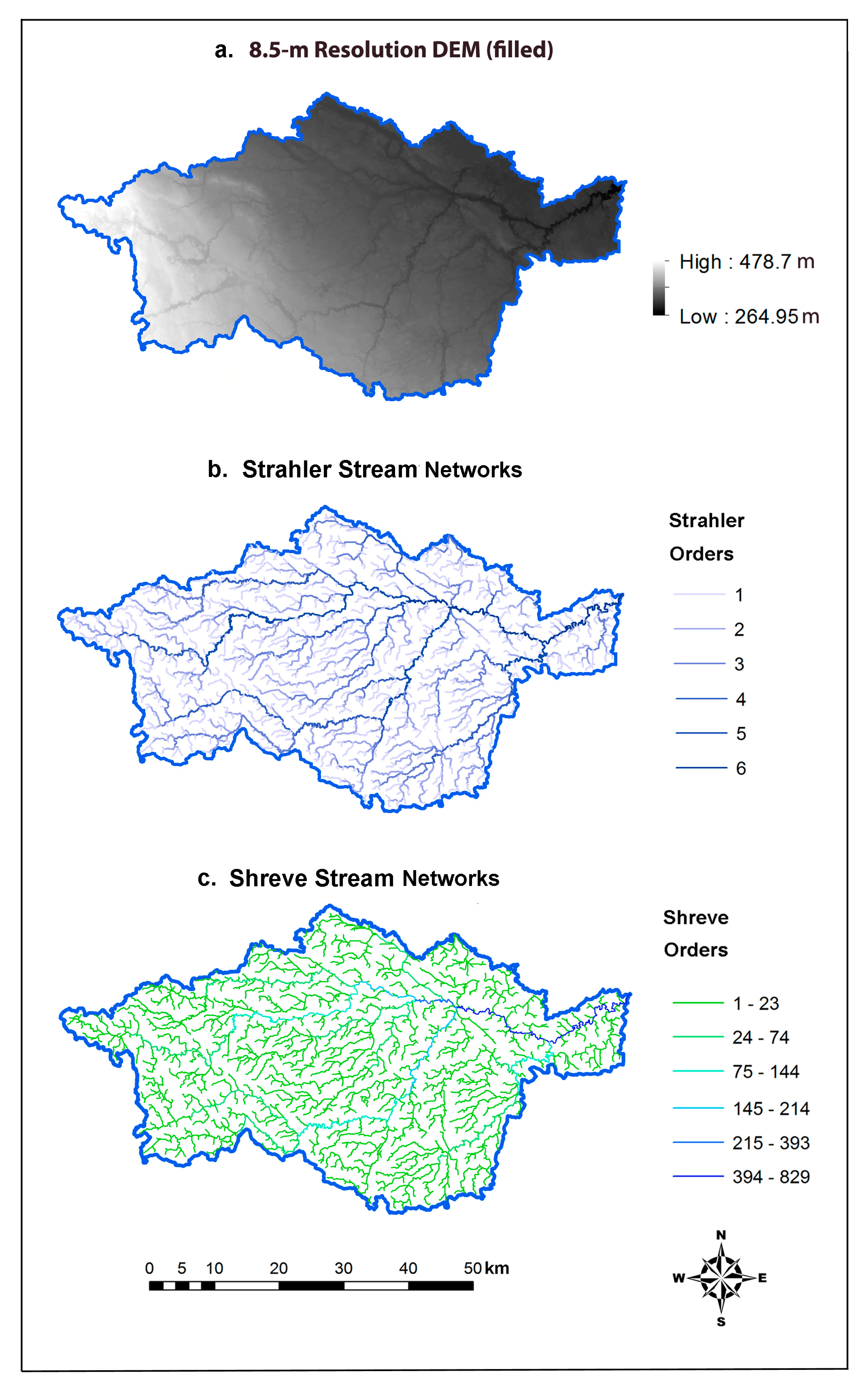
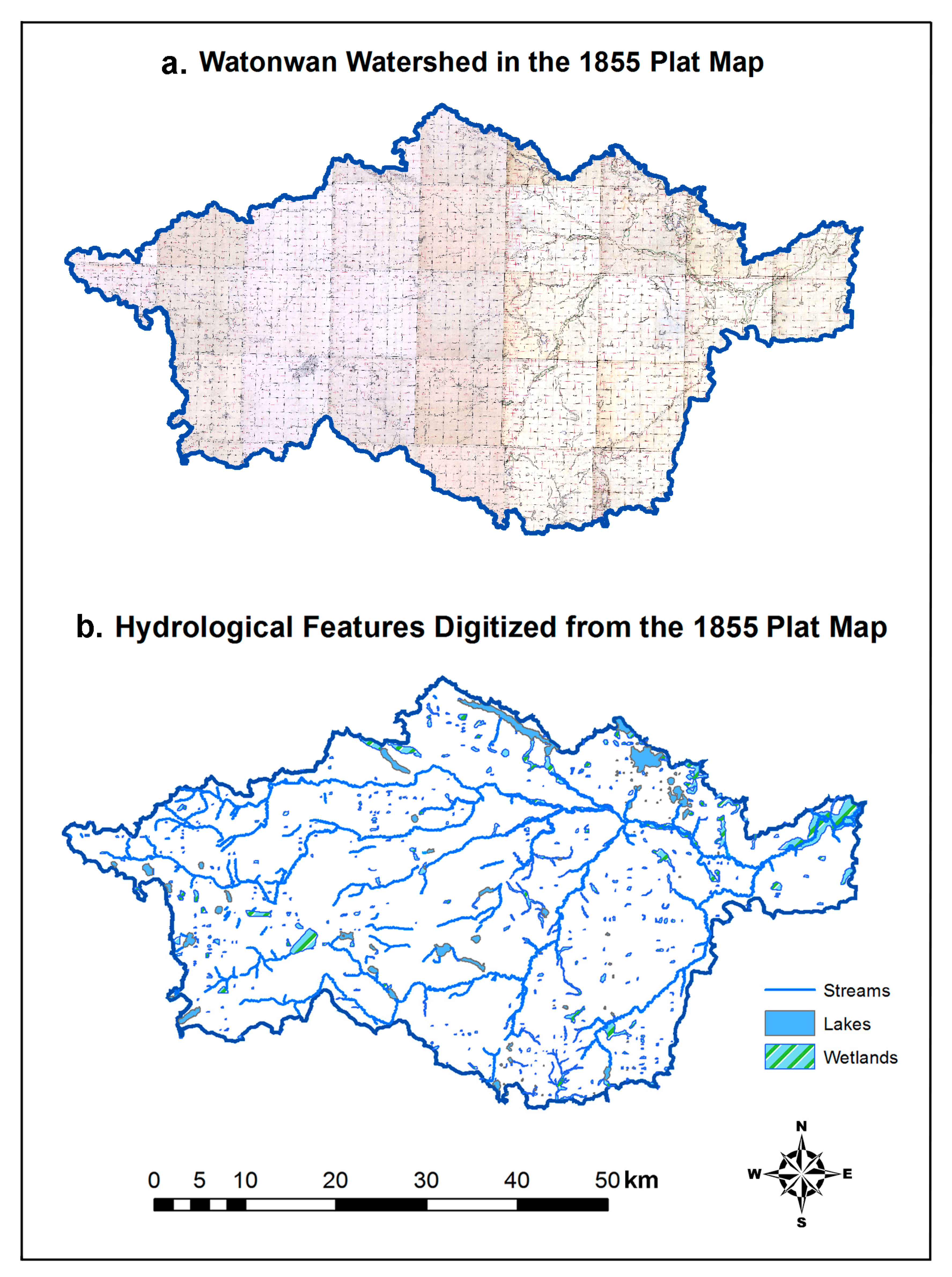
2.1. Historical Stream Network Derivation in Watonwan Watershed

A digital copy of Minnesota’s 1855 plat map imagery was obtained from the Minnesota Pollution Control Office (MPCA). The original hard copy plat maps were created between 1848 and 1907 during the first government land survey of the state of Minnesota by the US Surveyor General’s Office. The plat maps are on the Public Land Survey System (PLSS), and are divided by townships and sections. Each township is comprised of 36 sections, with an area of one square mile (640 acres or 259 ha) for each section. Distance was measured using chains and links, or using triangulation for those areas (e.g., lakes or hilly terrain) where measuring by chains was not possible (www.mngeo.state.mn.us/glo). The original map scale was 1:31,680 (1 inch = 40 chains). The scanned maps were of high quality (800 dpi; 24-bit color). For example, we were able to zoom into a scale of 1:4462, and the quarter section lines remained lucid on an 18 inch display. We could zoom in even further before encountering any fuzziness. Most of them were georeferenced in order to “coincide with statewide geographic data without appreciably altering (warping) the image” (https://gisdata.mn.gov/dataset/plan-glo-plat-maps-georef). Best available corners at the time to survey accuracy (1:24,000 scale) were used in the georeferencing process. First-order polynomial method was used. However, the number of ground control points (GCPs) and the root mean square error (RMSE) values for the rectification were not recorded. The survey plat maps and the survey field notes serve as fundamental legal records in Minnesota, as all property titles and descriptions for real estate transactions are based on these maps. In addition, they provide an underutilized “record of the state’s physical geography prior to European settlement” (www.mngeo.state.mn.us/glo/).

The digital plat map covering the Watonwan watershed was clipped from the statewide mosaic using the Watonwan watershed boundary file downloaded from the Minnesota Geospatial Commons (gisdata.mn.gov/). The plat map was then split into eight subsets to facilitate the accurate digitization of watershed surficial hydrologic features (e.g., streams, lakes, and wetlands). To locate the surficial hydrologic features, we utilized the PLSS township and section boundaries, the information shown on the plat map, and a map key from the Minnesota Geospatial Information Office (MNGEO). The hydrologic features were digitized at an approximate scale of 1:5000. A file geodatabase was created for each plat map subset, in which individual feature layers for streams, wetlands, and lakes were created. The attributes for all features in these individual geodatabases were formatted to contain the same data structure in order to facilitate the successful merging of the feature data after digitization. After merging, any overlapping features were clipped, and stream digitization accuracy was re-evaluated and edited.

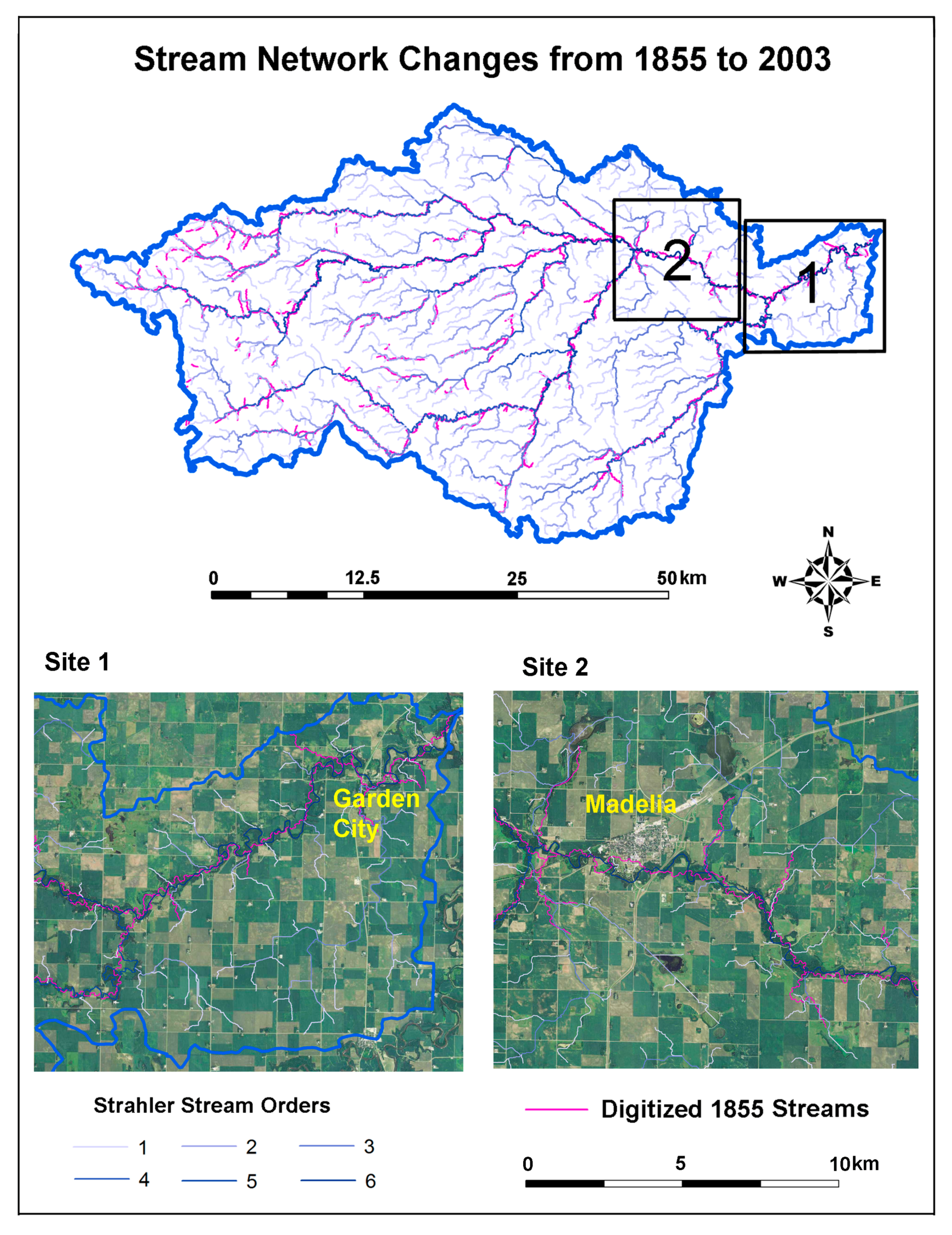
2.2. Contemporary Stream Network Extraction and Stream Change Analysis in Watonwan Watershed

While historical stream networks were digitized from the 1855 plat maps, contemporary stream networks were extracted from an 8.5 m resolution 2003 National Elevation Dataset (NED) obtained from the USGS (lta.cr.usgs.gov/NED). The NED DEM is a bare earth digital terrain model (DTM), and is in geographic coordinates with a North American datum of 1983. Using the hydrological tools in ArcGIS 10.3.1, a customized model was created to extract the stream network from the DEM. As DEMs usually contain depressions that hinder flow routing [17], the first step was to fill single-cell depressions in the DEM by raising each cell’s elevation to the lowest elevation value on the rim of the depression. This allows continuous water flows across the surface of the DEM within a watershed, and ensures water routes to a common outlet [19,20]. The filled DEM was then used to derive the flow direction and flow accumulation. Next, a stream network was created using a threshold value of 1000 cells based on the flow accumulation result. In particular, multiple thresholds (e.g., 500, 1000, 1500, 2000, etc.) were tested. Generally, the density of the drainage network decreases as the threshold value is increased. The threshold value of 1000 cells was selected as it provided an ideal result, with the extracted stream networks shown a high density and matched with the channel networks in the high-resolution digital aerial imagery. The resulting data were then applied to a stream order using both the Strahler [21] and Shreve [22] methods. Although commonly used, the Strahler method does have limitations, as it does not incorporate the cumulative increase in discharge that results from lower order tributaries flowing into larger order streams. Instead, the order only increases when streams of the same order intersect [21]. By contrast, in the Shreve method, the orders are additive. Thus, the numbers from the Shreve method indicate the numbers or magnitudes of upstream links [22]. In both methods, all stream links without any tributaries or upstream stream segments are classified as first-order streams.

To visualize and predict locations that have or may be undergoing stream network and geomorphic change (i.e., locations that are likely to have been or currently may be erosional point sources), the digitized 1855 plat map stream network was overlain on the 2003 streams extracted from the 8.5 m DEM. This was done so that a comparative analysis of stream network changes could be observed. In ArcGIS, the contemporary stream network characterized using Strahler stream ordering was intersected with the digitized 1855 network to delineate the changes in the stream network over this time period. Stream sinuosity values were calculated as the actual path length of the river divided by the shortest path length from the two times, and compared.

Other watershed scale datasets were obtained or derived to evaluate the contemporary physical and geomorphic characteristics of the watershed to predict where modern geomorphic/erosional processes may be most active. Percent slope and a topographic position index (TPI) were calculated across the watershed. TPI calculates the difference between the elevation at a cell, and the average elevation in a neighborhood surrounding that cell. Both percent slope and TPI were derived from the DEM using a 3 × 3 pixel neighborhood around the center pixel. Both metrics can indicate areas of high relief, where fluvial and hillslope geomorphic processes may be intensely active on eroding banks, bluffs, and ravines (1). In addition, the 2011 National Land Cover Data (NLCD) was downloaded from the Multi-Resolution Land Characteristics (MRLC) Consortium (www.mrlc.gov/nlcd2011.php), and extracted for the Watonwan watershed. The NLCD data is used to assess the character of current land use at the watershed scale. This is particularly important, as it has been suggested that the conversion of native wetland and prairie to row crop agriculture is correlated to the dynamic change responsible for growing environmental issues in the regional waterways [23]. The 1855 plat maps were created before the most significant shifts in land use practice in the region.

The Soil Survey Geographic Data (SSURGO) was downloaded from the United States Department of Agriculture (USDA) Geospatial Data Gateway (gdg.sc.egov.usda.gov/) for each of the six counties covering the watershed. They were then merged and clipped using the Watonwan watershed boundary file. From the soil dataset, hydrological soil groups and the soil erodibility factor (K-factor) values were extracted and mapped to estimate areas prone to erosion and the relationship of these areas to soil characteristics. Specifically, hydrological soil groups include four types: “A”, “B”, “C”, and “D”, with the “A” soil type representing the highest rate of infiltration [24]. The K-factor indicates the relative susceptibility of the soil to erosion, and the amount and rate of runoff [25]. It ranges from 0.02 for the least erodible soils to 0.64 for the most erodible [26]. According to the USDA [23], fine textured soils that are high in clay have low K values (<0.15), as they are resistant to detachment. Coarse-textured sandy soils also have low K values (<0.2) because of low runoff, even though they are easily detached. Medium-textured soils (e.g., silt loam soils) have moderate K values ranging from 0.25 to 0.4. Soils with a high silt content are the most erodible (K values >0.4), as they are easily detached, and tend to produce large amounts and rates of runoff.

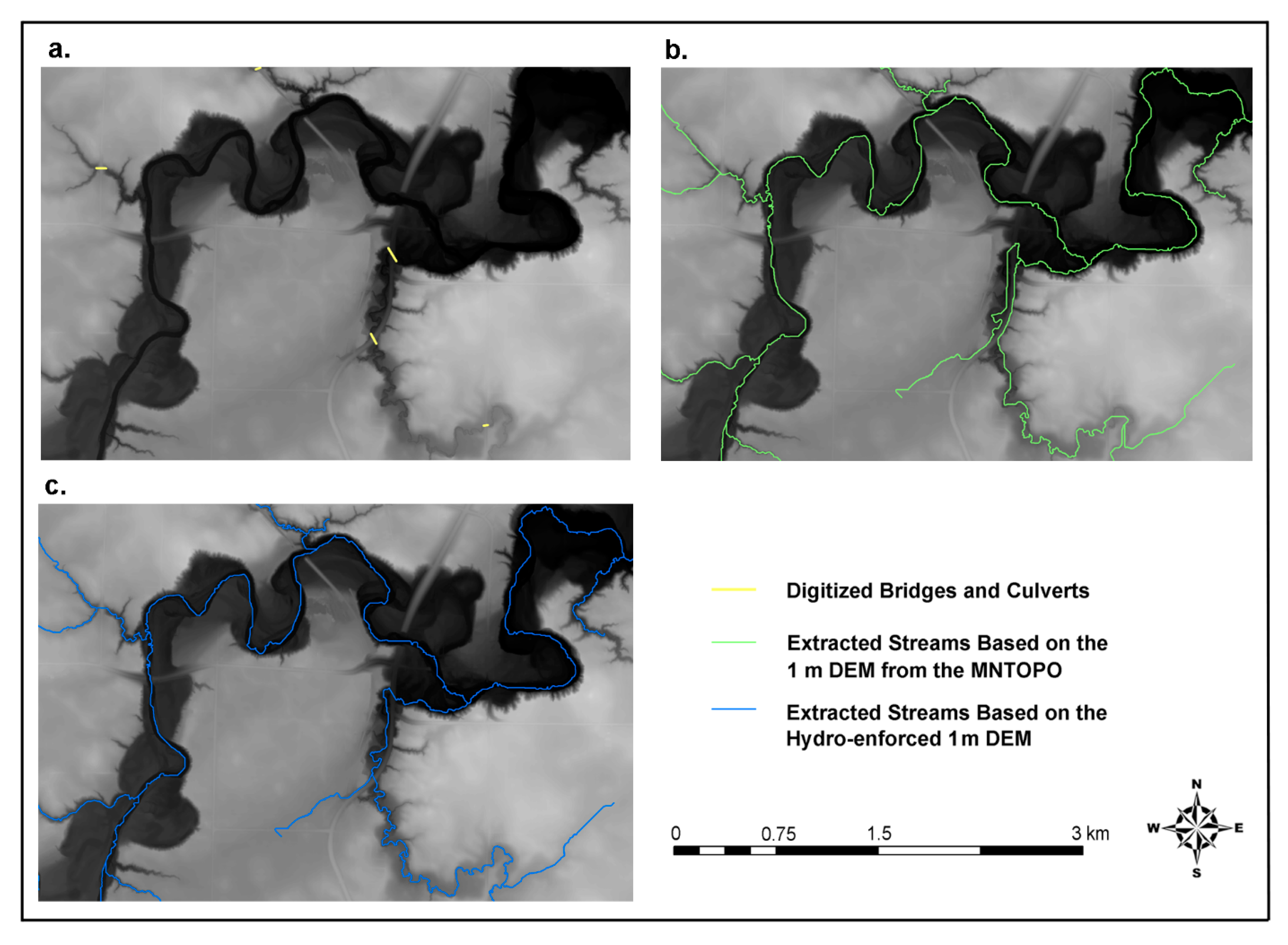
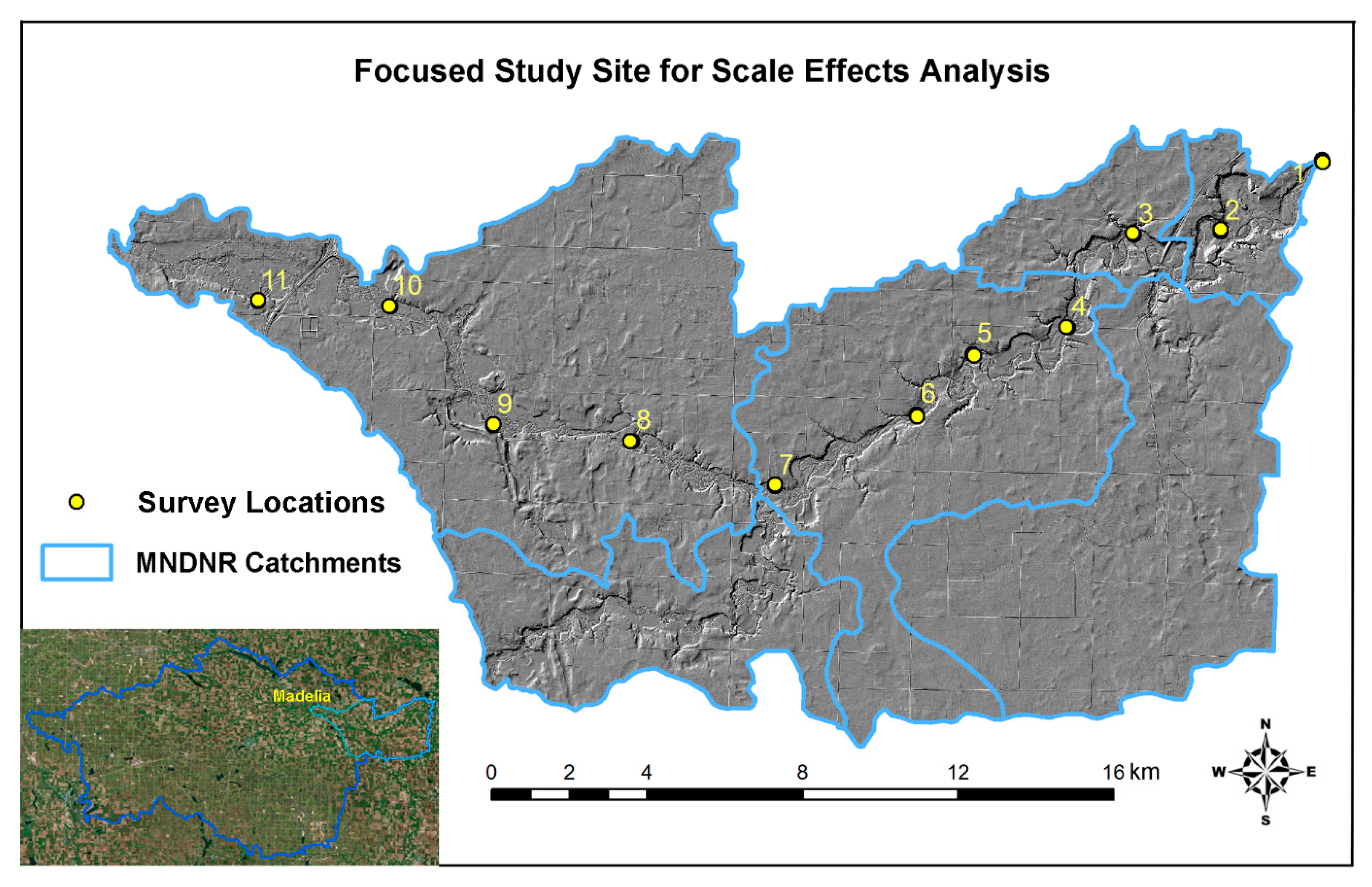
2.3. DEM Scale Effect Analysis and Creation of Hydrologically Enforced LiDAR-based DEM in a Focused Study Site

To evaluate how the spatial resolution of a DEM may affect the accuracy of an extracted stream network, scale effect analysis was conducted using multi-resolution (1 m, 3 m, 8.5 m and 30 m) DEMs for a focused study area—six Minnesota Department of Natural Resources (MNDNR) catchments along a 32 km (20 mile) stretch of the east Watonwan River, starting from the city of Madelia (Figure 2). MNDNR catchments are the smallest delineated and digitized drainage areas representing the hydrologic boundary [27]. The average drainage area of the six catchments was 3653 ha. While the 8.5-m and 30-m DEMs of 2003 were obtained from the USGS (lta.cr.usgs.gov/NED), the 1-m and 3-m DEMs were downloaded from the MnTOPO (arcgis.dnr.state.mn.us/maps/mntopo/), which is a web application for viewing and downloading Light Detection and Ranging (LiDAR)-based high-resolution elevation data, made available by the Minnesota Elevation Mapping Project of the MNDNR. The LiDAR data covering this study site was acquired between 2010 and 2012. There was a seven to nine year gap between the LiDAR data and the USGS DEM. During that intervening period, there were no catastrophic events. Our findings of nominal changes in the river course during this period serves as corroborating evidence.

Before extracting the stream network, the high-resolution LiDAR-based 1-m and 3-m DEMs covering this focused study area were further hydrologically modified using the Agricultural Conservation Planning Framework (ACPF) tool provided by the USDA. As an extension to ArcGIS software, the ACPF tool is designed to process and analyze soils, land use, and LiDAR-based high-resolution elevation data in order to identify a broad range of opportunities to install conservation practices in fields and/or in HUC12 subwatersheds (http://northcentralwater.org/acpf/). The ACPF tool has the hydromodification functions. There are four levels of DEM hydromodification: (1) the level 1 hydro-smoothing development fills and/or breaches depressions across the DEM landscape simply to make water flow to a hydrologic point of interest, as we did in the watershed-scale stream network extraction using the 8.5-m DEM in Section 2.2. DEMs of this level are the least accurate at representing actual landscape hydrology, because the elevation alterations are conducted on the DEM without regard to the scope and scale of subsequent user needs; (2) the level 2 hydro-flattening process is the standard LiDAR-based data holding for Minnesota disseminated through the MnTOPO website. The LiDAR-derived bare earth elevation values from the source data remain intact, except at selected influential large bridge decks and within the confining boundaries of lakes and streams. Using LiDAR data, terrain drape, and/or 2D digitization, breaklines can be created to flatten the lakes and open water wetland elevations to a constant elevation. For example, the LiDAR-based 1-m and 3-m DEMs downloaded from the MnTOPO are hydro-flattened by vendors; (3) In the level 3 hydro-enforcing development, major road–stream crossings are breached for DNR mapped watercourses using breakline enforcement to allow the DEM surface to depict the actual flow of water beneath the roads; and (4) in the last level of the hydro-conditioning process, all DEM depressions in a watershed are evaluated with the greatest cost in order to replicate landscape hydrology and hydrologic connectivity across a drainage area of interest while maintaining the integrity of the DEM [28].

To extract accurate stream networks from the LiDAR-based DEMs in this study, the third level hydromodification (hydro-enforcement) is preferred. In the analysis, the major road–stream crossings for the test study site were manually breached on the screen using the Minnesota Department of Transportation (MNDOT) bridges and culverts point feature layer and the MNDNR’s hydro-infrastructure’s layer as the references. Consequently, the 1-m and 3-m DEMs were hydro-enforced using the digitized breaklines in the ACPF tool before the stream network extractions.

Due to the limitations and technical challenges discussed in the Supplementary section, we were only able to conduct the hydro-enforcement for the LiDAR-based DEMs in a focused study area, which equals about 9.64% of the total area of Watonwan watershed.

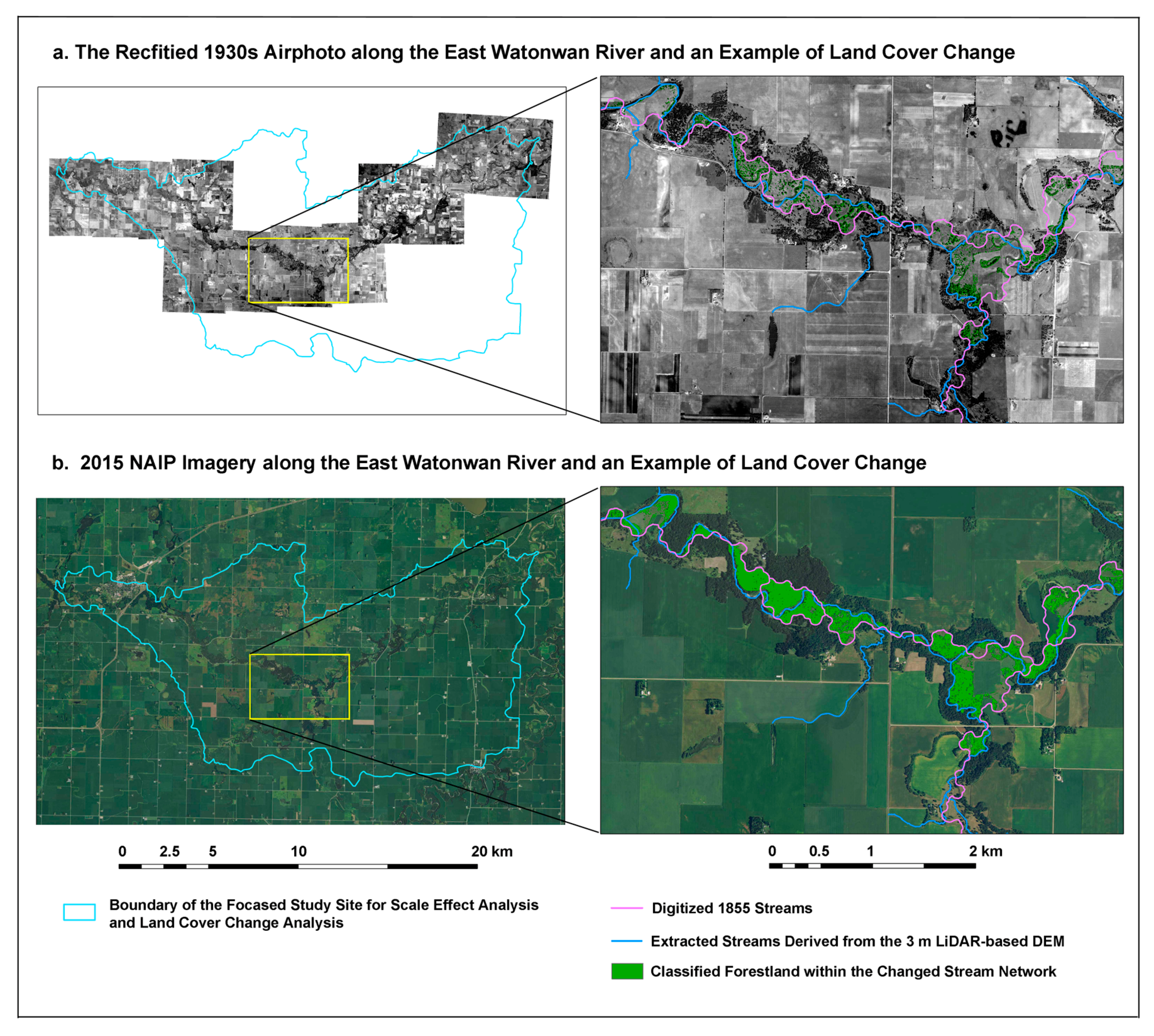
2.4. Field Survey and Land Cover Change Analysis in a Focused Study Site

A field survey was also conducted to assess river widths and river centers at 11 field survey locations that were roughly evenly distributed along the 32-km stretch of the East Watonwan River (Figure 2). A Trimble Geo7x GNSS (Global Navigation Satellite System) unit was used. The GNSS plotted points along the river have gone through differential corrections, but have also produced results with a majority accuracy of 1–2 m due to the presence of dense tree canopies along the river. To determine river width at each survey site, the left and right bank points were measured separately using the GNSS and then measured by connecting them in ArcGIS. Consequently, the center of the river channel was identified and measured for the 11 sites by bisecting the connected lines. The accuracies of the stream networks extracted by the customized GIS model, from four DEMs of different resolutions, were assessed using the GNSS measured locations and the 1-m resolution 2015 National Agricultural Inventory Program (NAIP) aerial imagery.

We utilized 2011 NLCD data for the entire watershed-level land cover analysis. However, the earliest available NLCD data was only from 1992. Therefore, to evaluate the long-term land use change and further examine the land-use changes within the stream network, historical high-resolution aerial images and contemporary NAIP orthoimagery were used. The historical, 1930s 1-m resolution black and white (B&W) aerial photographs were acquired from the Minnesota Historical Aerial Photographs Online database (www.lib.umn.edu/apps/mhapo/). The 2003 and 2015 color NAIP orthoimagery with red, green, and blue bands were acquired from the MNGEO Data Clearinghouse (www.mngeo.state.mn.us/). To cover the 32-km main stem of the east Watonwan River, in total, 12 scanned aerial photos from the 1930s were obtained, while the contemporary NAIP images were obtained as county mosaics. Aerial photo collections and interpretations were focused on identifying significantly changed areas along the river.

The historical photos were georectified individually using the 2015 NAIP imagery as the reference map. The map scale of the 1930s B&W photos is 1:20,000 while the color NAIP orthoimagery have a nominal scale of 1:40,000. For each aerial photo, 10 GCPs (e.g., road crossings or artificial targets) evenly distributed across the photo were identified and collected. No camera calibration parameters were used, as we did not have access to this information. The RMSE values were less than 3 m. The 12 rectified aerial photos were then mosaicked together. The land-use and land-cover changes within the identified changed stream network along the 32-km stretch of the Watonwan River were examined by classifying the 1930s historical aerial photos and the 2015 NAIP imagery. Feature Analyst, an object-based classifier that makes use of not only spectral, but also spatial information in the imagery, was used. It was found that for remote sensing images with a low spectral variation, especially for the historical B&W aerial photography, the object-based approach and hierarchical learning process provided by the Feature Analyst were very useful [29,30]. Training polygons for forest and agriculture land-cover classes were carefully digitized from the high spatial resolution airborne imagery for both years, as they are the two prevailing land-cover types shown in the changed areas of stream networks.

3. Results

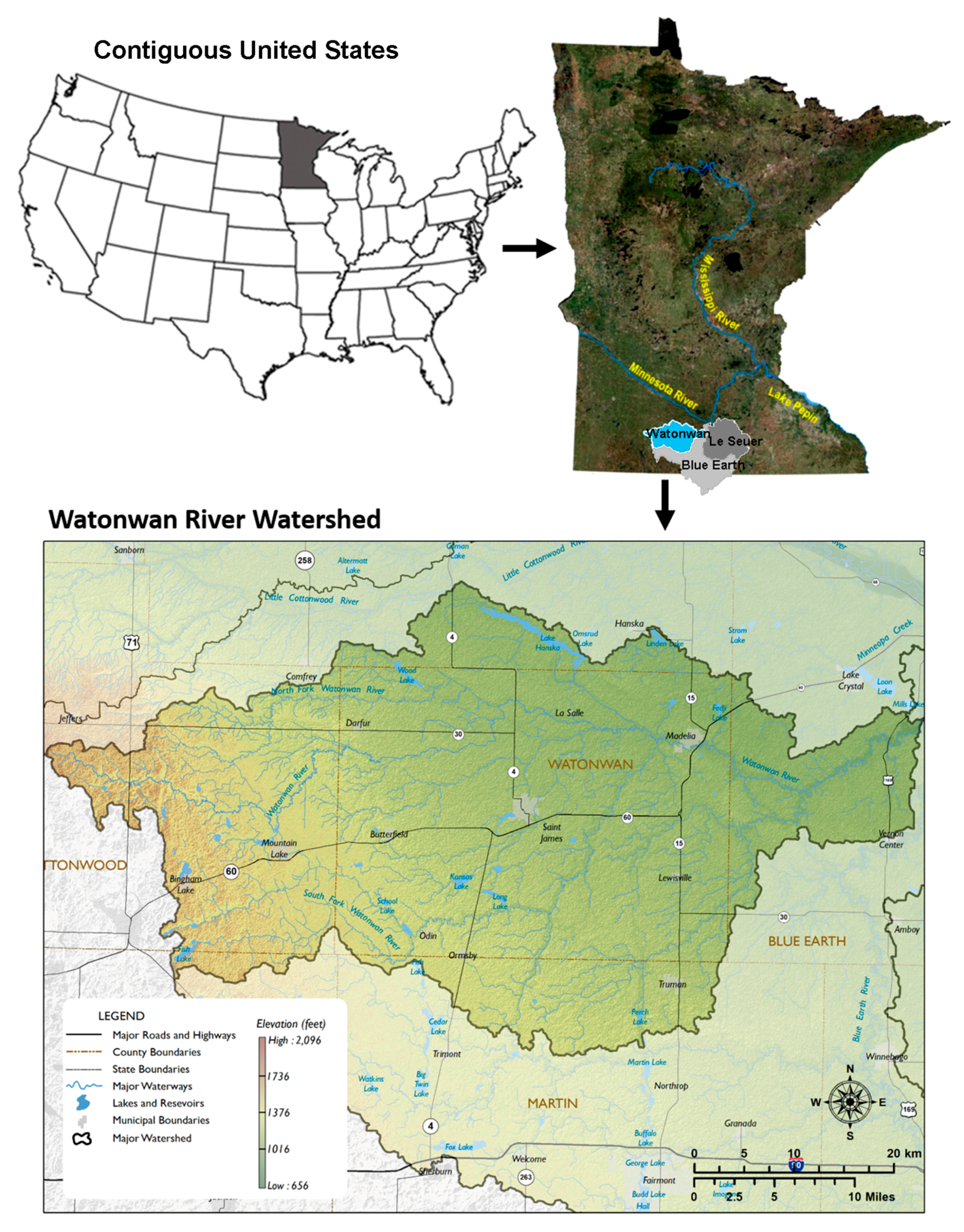
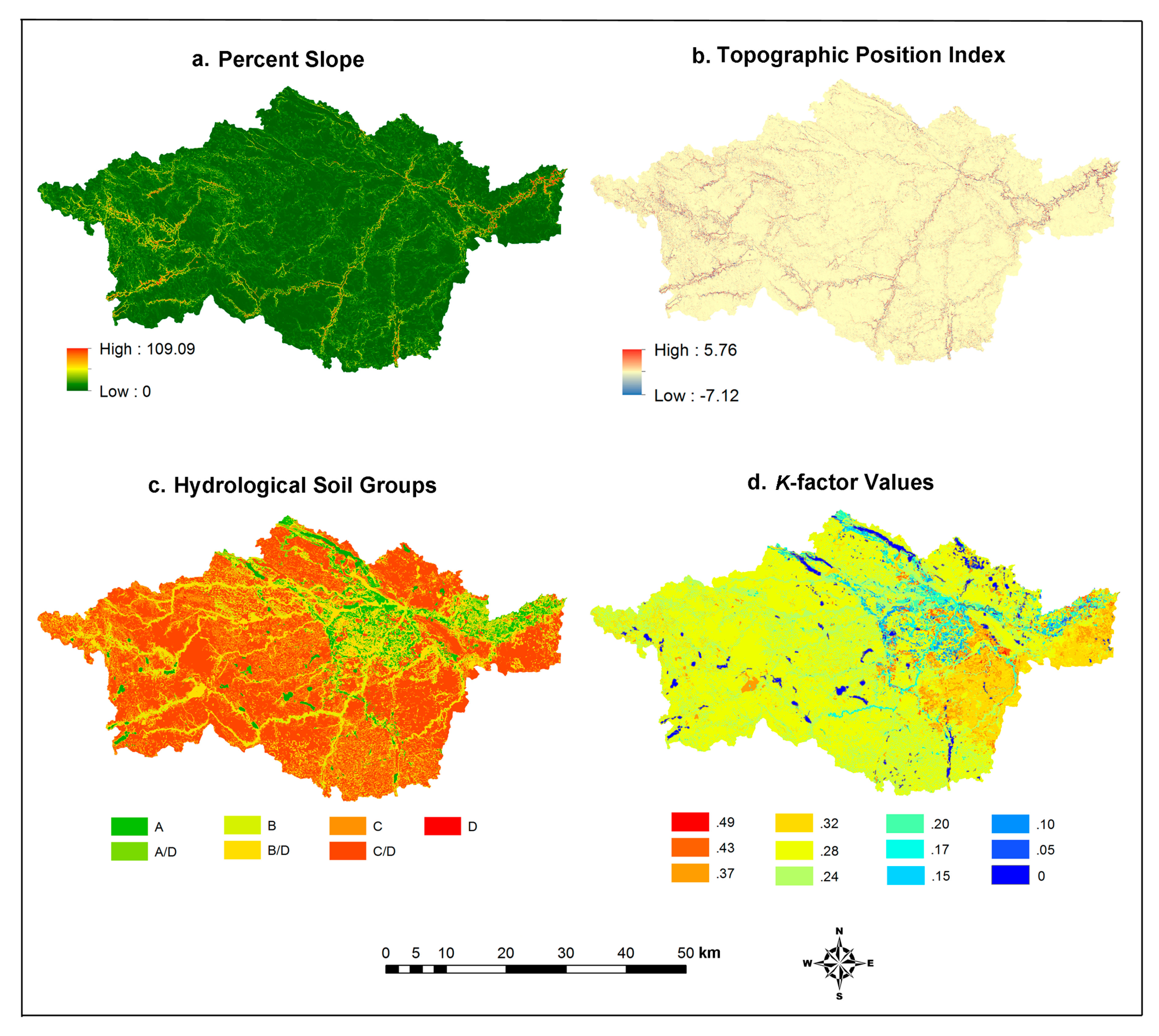
3.1. Geomorphic Characteristics of the Watonwan Watershed

The calculated percent slope map of the entire watershed revealed ranges from 0 to 109.09%, or 0 to 47.49 degrees, with the highest slopes concentrated in the lower ~20 km of the watershed (Figure 3a). The calculated TPI also revealed similar spatial patterns to the percent slope data within the Watonwan watershed (Figure 3b). SSURGO data indicated that the majority of the watershed is underlain by low permeability hydrological soil types (C, C/D, D), with only small clusters of highly permeable (A and B) soil groups located primarily in the northeastern and north–central reaches of the watershed (Figure 3c). C and D hydrologic soil groups, which predominate the watershed, have moderate to high surface runoff potential, contain 20–40% (C) or >40% (D) clay content, and <50% sand [25]. The soil erodibility (K) values range from 0.05 to 0.49 in the watershed (Figure 3d). However, the majority of the watershed has moderate or high K values ranging from 0.28 to 0.49, likely indicating high silt loam and/or silty-textured soils. The locations with the highest K-factor values in the eastern Watonwan watershed also, generally, have the most impermeable soil types (C and D).

3.2. Hydrogeomorphic and Land-Cover Changes

The 8.5-m DEM and the derived contemporary stream networks in Strahler and Shreve orders are displayed in Figure 4, while the digitized 1855 plat map hydrology is displayed in Figure 5. Through comparative analysis, we found that the Watonwan River channel has straightened along many segments close to small towns and at some areas of confluence with tributary streams (e.g., Figure 6). For example, Garden City and Madelia are two such small towns (Figure 6). We observe the overall course of the Watonwan River being changed significantly between 1855 and 2003. The measured maximum river course shift is approximately 740 m near Madelia, as shown in Figure 6. The minimum measured shift was 2 m. The sinuosity of the digitized 1855 Watonwan River channel ranges from 1.08 to 6.76, with an average of 1.57, whereas the sinuosity of the 2003 third to sixth order (Strahler) streams is from 1 to 2.98, with a mean value of 1.44.

According to the 2011 NLCD data, nearly 87% of the Watonwan watershed’s land use was in “Cultivated Crops”, followed by “Developed, Open Space” (5.23%) and “Emergent Herbaceous Wetlands” (2.65%) (

Table 1. 2011 National Land Cover Data (NLCD) statistic for the Watonwan watershed.

Land Cover Class	Total Area (ha)	Percentage (%)
Cultivated Crops	195,898	86.57
Developed, Open Space	11,835	5.23
Emergent Herbaceous Wetlands	5947	2.63
Open Water	3583	1.58
Deciduous Forest	2434	1.08
Grassland/Herbaceous	2080	0.92
Developed, Low Intensity	1627	0.72
Pasture/Hay	1185	0.52
Other Land Covers	1693	0.75

). Figure 5 shows the 1855 plat map and the digitized historical hydrological features including streams, lakes, wetlands, and rivers in the Watonwan watershed. Lakes and wetlands were mainly concentrated in the northern and northeastern portions of the watershed. When compared with the lakes and wetlands extracted from the National Wetlands Inventory (NWI) (http://www.fws.gov/wetlands), we found that many wetlands were diminished, conforming to the MPCA [13]’s report that the wetlands in the Watonwan watershed have been reduced by 92%.

Furthermore, land-cover change analysis along the main stem of the east Watonwan River, a 32-km reach in our focused study area, revealed that in the 1930s, land cover was approximately 15% forest and 84% agriculture land; however, the land-cover composition changed significantly, with 51% forest and 47% agriculture found in 2015 (Figure 7).

3.3. DEM Scale Effect Analysis Result for the Focused Study Site

Figure 8a provides an example of the breached digitized dams (road–stream crossings) overlaid on the 1-m LiDAR-based DEM obtained from the MnTOPO website. The extracted stream networks from the original 1-m DEM and the hydro-enforced 1-m DEM are shown in Figure 8b,c. Our results indicate that the hydrological enforcement allowed the actual flows of water beneath the road at mapped intersections of roads.

The accuracies of the stream networks extracted based on the four DEMs of different resolutions were assessed by calculating the distances between the measured river center using the global positioning system (GPS) unit and the extracted river center by the GIS model at the 11 survey sites. The results are summarized in

Table 2. Measured river widths and accuracy assessment of the extracted river centers derived from the four different DEMs at the 11 sample sites.

Field Sample	River Width (m)	Distance Between Extracted River Center and Measured River Center (m)
		1-m DEM	3-m DEM	8.5-m DEM	30-m DEM
1	44.96	13.33	14.31	0.48	788.35
2	44.46	12.66	10.98	12.74	67.47
3	36.24	11.22	10.58	10.52	22.57
4	38.48	10.40	7.88	20.39	4.69
5	39.55	14.93	14.20	12.55	19.54
6	37.74	15.79	15.82	40.32	53.51
7	36.88	12.74	14.76	30.52	40.23
8	38.81	3.35	0.36	28.14	61.56
9	22.80	1.89	5.90	6.38	329.17
10	20.68	41.90	47.72	7.29	605.61
11	25.96	11.54	6.54	9.89	37.76
Mean	35.14	13.61	13.55	16.29	184.59

, from which we can see that the LiDAR-based 1-m and 3-m DEMs produced the most accurate streams, with a mean error of approximately 13.6 m. The streams created from the 8.5-m DEM showed a slightly higher distance error of 16.3 m. In contrast, the mean distance between the extracted river center and measured river center derived from the 30-m DEM is remarkably larger (184.59 m), with sample site #10 showing the highest error of 605.6 m.

Our scale effect analysis in the focused study site showed that the 3-m DEM achieved similar accuracy to the 1-m DEM, indicating that the 3-m DEM might be the optimal input for HUC12 subwatershed-scale or MNDNR catchment-level hydrological analysis. On the other hand, the streams created from the 8.5-m DEM showed only a slightly higher error than those of the 1-m and 3-m DEMs. These results demonstrated that for HUC8 watershed-scale analysis, it is practical to use the 8.5-m DEM when also considering the tolerance fault issue (described in the Supplementary section) related to watershed analyses using high-resolution DEMs.

Moreover, to extract highly accurate high-resolution stream networks, it is necessary to develop a hydro-enforced DEM manually using the ACPF tool by breaching major road–stream crossings using breakline enforcement to depict the actual flow of water beneath the roads. In addition, when comparing the streams produced from the hydrological model based on the 8.5-m DEM to the high-resolution NAIP orthoimagery, it was found that the model is most accurate in the west portion of the watershed. This is probably due to there being less variation in elevation, while the east portion of the watershed could have benefitted from a higher resolution DEM. This was confirmed by the results based on the 1-m and 3-m hydro-enforced DEMs for the selected catchments on the east Watonwan River. The MNDNR is working on producing a hydrologically enforced LiDAR-based DEM for the entire Watonwan watershed. Upon completion, this product would greatly benefit various local hydrological studies. For example, the hydro-enforced product can be resampled to 8.5 m resolution and used to extract a more accurate stream network for the entire Watonwan watershed, as the hydro-enforced LiDAR provides better positional accuracy.

4. Discussion

In general, altered hydrology seems to define the hydrology of the Watonwan River watershed, as only 22% of streams have not been modified in the watershed ([13]; Figure 4 and Figure 5). According to the MNDNR [16], “significant portions of the river and its tributaries have been straightened and altered to provide for drainage of farmland and flood reduction.” For example, the North Fork Watonwan River, starting in the northwest corner of the watershed, has been channelized through the reach between 1950 and 1991, whereas the Lower Watonwan River near Garden City is over-widened, not accessing its floodplain until bankfull flow is more than doubled [16]. We do observe significant change along the main stem of the Watonwan River through this historical period. The river does reveal a high degree of lateral mobility between 1855 and 2003 (up to 740 m; Figure 6); however, where now controlled, the channel will likely no longer vary its course to this degree. The measured reduction in sinuosity further supports that assessment.

The reduction of lateral migration of the Watonwan River and of the frequency of wetlands throughout the watershed reduces natural floodplain development and water storage in the watershed. This creates a flashier system, and consequently leads to shortened time-to-peak discharges, and exacerbates flooding issues in the watershed [13,17]. Furthermore, the Watonwan River watershed rates poorly for stream connectivity to riparian land, leading to increased bank erosion and more sediment entering the stream [13,31]. As there is a significant rising trend of precipitation in Minnesota, including the Watonwan watershed in the past 100 years [13,32], the erosion and flooding issues may become more severe over time.

Recent research [1,15] has pointed to near-channel sources (i.e., exposed bluffs, channel banks, river incisions, and ravines) as the primary source of suspended sediment loading in the Le Sueur River basin, a neighboring fluvial system to the Watonwan River watershed. An innovative geochemical fingerprinting methodology and multi-temporal sediment budget was used to identify and trace the sources of sediment loading and elucidate on the rates of erosional processes within that watershed. Given the similar geomorphic/geologic/landscape history of the Le Sueur and Watonwan Rivers [5], it is likely that similar types of point sources occur in both watersheds. Although their methodology was effective at identifying point sources of concern and characterizing the relative importance of different erosional processes by utilizing their representative sample sites, it was beyond the scope of that work to paint a complete picture of the spatial distribution, at a watershed scale, of these areas of concern, or to map and locate distinct spatial reaches prone to these erosional processes.

In the Watonwan watershed, limited spatial data exists to visualize areas of potential concern as well. In this work, we demonstrate that identifying the spatial distribution of areas of susceptibility to erosional processes in these watersheds may be possible through the compilation of a number of geospatial datasets (Figure 3a,b,d). For example, areas of high slope and high TPI (Figure 3a,b) represent the areas of highest relief in the watershed. These areas of highest relief are located in the eastern portion of the watershed as a result of the incision of the Watonwan River, similar to other rivers in this northernmost reach of Blue Earth watershed, into the surrounding landscape. An actively propagating knickzone has developed through these watersheds in response to abrupt base-level fall of the Minnesota River valley that occurred approximately 13.4 k.y. B.P. [5]. This higher relief area, similar to the neighboring Le Sueur River basin [1,15,33], is most likely where the majority of sediment loading occurs. In addition, areas of high soil erodibility, based on K-factor values [34], can be compared with areas of high relief to further indicate the areas with the highest potential for erosive processes to occur (Figure 3a,d).

Other recent work [2,3] has demonstrated an order of magnitude shift in sedimentation rates in depositional sinks (e.g., Lake Pepin, Figure 1) downstream of the Watonwan River. However, our understanding of the historic dynamics and characteristics of the watersheds responsible for transporting this sediment are not well developed. In this novel approach, we observe land-use change from more abundant wetlands mapped on the 1855 plat maps (Figure 5) to more abundant crop land and wetland reduction (Table 1). This transition from the 1855 plat map to modern land-use imagery coincides with the onset of commercial agriculture in the region [2]. In addition, more recent “agriculture to forest” land conversion (Figure 7) along the river might be attributed to the Conservation Reserve Program (CRP), a cost-share and rental payment program signed into law in 1985 and administered by the Farm Service Agency (FSA) under the USDA. Through the implementation of 10-year contracts paying annual rents, the CRP aims to counteract erosion and protect the environment by encouraging agricultural landowners to convert highly erodible cropland and other environmentally-sensitive lands to native or alternative permanent vegetative cover [35]. The CRP in Minnesota mainly concentrate in the Minnesota River basin and the Red River Valley, with an enrollment of 780,262 ha (1.9 million acres), 576,698 ha (1.4 million acres), and 447,194 ha (1.1 million acres) in 1993, 2005, and 2014, respectively [35]. In addition, the Conservation Reserve Enhancement Program (CREP) was established in 1998 as a subprogram of the CRP to enhance water quality and wildlife habitat. It is a joint federal (USDA) and state program aimed at retiring 40,469 ha (100,000 acres) in the Minnesota River basin using long-term (14–45 years) or permanent conservation easements [36]. Yuan et al. [35] examined the land-cover change in the Minnesota River Valley from 1985 to 2013. They found that 36,000 ha cropland within a 1.6 = km (1 mile) buffer of the Minnesota River has been converted to grassland or forestland. The land-cover change result of this study conforms to Yuan et al. [35]’s finding. The result is also in conformity with the report by the USDA Natural Resources Conservation Service (NRCS) [37], which noted that 2385 ha (5893 acres) and 2236 ha (5525 acres) cropland in the Watonwan watershed were enrolled in the CRP and the CREP, respectively.

We also observe substantial stream network change along the largest channels in the watershed, where the locations of the 1855 stream networks can be directly associated with 2003 DEM-derived networks (Figure 6). In the main stem of the Watonwan River, we observe a maximum of 740 m and minimum of 2 m of lateral movement, indicating a substantial reworking of floodplain sediments and erosion into channel banks and nearby bluffs in certain portions of the river. Future work could aid in identifying point sources through further aerial photo interpretation and ground/field based reconnaissance of the watershed. Monitoring sites could be established to determine process rates and sediment budget, similar to Gran et al. [16]. Lastly, it is important to note that the 1855 plat map was not well suited for identifying the locations of smaller tributary systems (first, second order). Much of the overall network scale analysis was not possible, revealing the limitations of this dataset in providing watershed stream network analysis. Future research could expand on this methodology with more thorough stream network analysis through the digitization of channels from each year of aerial photographs available in this watershed. Then, a more comprehensive analysis of change through time could be assessed.

5. Conclusions

In this study, hydrologic features were successfully digitized from the 1855 GLO plat maps. The natural stream networks and stream orders were successfully extracted from the USGS 8.5-m DEM in a watershed scale. It was found that many water bodies changed since 1855, and the main stem of the Watonwan River has been straightened along many of its segments and at tributary confluences. The areas most susceptible to erosion are located in parts of the eastern portion of the Watonwan watershed, where high soil erodibility values and substantial relief derived from a propagating knickzone sets the stage. In addition, major land-cover conversion began with a reduction of wetlands, as observed in the 1855 plat map, in favor of agricultural land use. More recently, the area underwent a shift from “agriculture to forest” within the river valley corridors, indicating the policy effect of using a CRP to counteract erosion and enhance water quality in the Minnesota River system. While the 8.5-m DEM is suitable for hydrological studies such as this at the watershed scale, the stream networks produced from a 30-m DEM could have significant locational displacement. The scale effect of analysis also indicated that for subwatershed-level hydrological analysis, the hydrologically-enforced LiDAR-based high-resolution (1–3 m) DEMs would provide the most accurate results.

Stream network change reveals the planform “shifting” of an entire fluvial system through time, both via natural and anthropogenic processes. Future work to further refine this analysis can aid in our understanding of near-channel sediment sources and the rates of erosional processes occurring within the watershed to facilitate mitigation and preventative policy. Future analysis would benefit from not only using the 1855 plat maps, but also from digitizing stream networks through the entire period using aerial photographs or other geospatial datasets. Results from this sort of research can aid in our understanding of watershed-scale past and present geomorphic and hydrologic changes over time. Changes in the main Watonwan River will continue to be monitored in the future to understand the river’s hydrogeomorphic evolution and water quality conditions.

6. Supplementary Materials: Methodological Challenges

Even though the original land survey plats were drawn with essentially standardized symbology, styles vary, as each map was hand drawn. Determining the difference between surficial hydrologic features such as wetlands, marshes, and lakes from the plat maps was sometimes difficult, especially when the map legends did not adequately describe all of the features shown on the maps, and/or when the symbology used in the plat maps was small or poorly illustrated, making it difficult to interpret. Another challenge encountered was the plat maps were mosaicked maps, and the lines did not match on the edges for each PLSS section. Therefore, some manual interpretation and editing were required when digitizing features across multiple plat maps. In addition, the study site was large (226,205 ha). Digitizing all of the water features from the plat map was time-consuming. Consequently, data layers digitized from plat maps were done with multiple analysts to save time. The digitized features were merged, and some overlapped features were cleaned up.

Although we streamlined the process of extracting watershed-scale stream networks from the 8.5-m DEM, it still took hours to run the model on a computer with a 16 gigabyte RAM and a processor of Intel(R) Core(TM) i7-5600U [email protected] GHz. At the watershed-scale, the customized GIS model was also tested using the LiDAR-based 3-m DEM as the input. The Fill tool worked, as did the Flow Direction tool (finished in about 40 minutes); however, the Flow Accumulation process took much longer (multiple hours). However, the stream link function (from the Hydrological Toolset of ArcGIS) in the model was not able to finish, due to a tolerance fault caused by the extensive hydrological network for the watershed in the high-resolution 3-m DEM. Likewise, the USDA Natural Resources Conservation Service (NRCS) Engineering tool and the ACPF tool were tested for the watershed-scale stream network extraction using the 3-m DEM. The same issue occurred. It is known that the NRCS Engineering Tool has a processing error for large watershed somewhere around 6070 ha (15,000 acres) if a high-resolution DEM is used. Similarly, the ACPF tool is designed for HUC12 subwatershed-scale rather than HUC8 watershed-scale analysis. Such test results demonstrated that when using LiDAR-based high-resolution (1-m or 3-m) DEMs as the input, all three aforementioned tools are limited to the subwatershed-scale analysis.

Furthermore, the USGS 8.5 DEM for the entire watershed was filled using the standard ArcGIS tool, whereas the LiDAR-based DEMs for the focused study site were filled and hydro-enforced using the ACPT tool. The reason we used two different tools is because the ACPF tool is designed specifically for LiDAR-based DEM processing for HUC12-size subwatersheds, rather than HUC8-size watersheds. The ACPF tool provides four levels of hydromodification functions for LiDAR-based DEM. “Filling the depressions” is just the level one processing. Therefore, for HUC8 watershed level analysis, we used the standard ArcGIS tool to fill the 8.5-m DEM. For subwatershed/catchment level analysis, we used the ACPF to process the LiDAR-based DEM to level three of the hydro-modification product. ACPF was chosen because high-resolution LiDAR-based DEMs are more sensitive to aboveground noises such as road–stream crossings/bridges, which need to be removed before they are used in stream network extraction.

References

1. Belmont, P.B.; Gran, K.B.; Schottler, S.P.; Wilcock, P.R.; Day, S.S.; Jennings, C.; Lauer, J.W.; Viparelli, E.; Willenbring, J.K.; Engstrom, D.R.; et al. Large shift in source of fine sediment in the Upper Mississippi River. Environ. Sci. Technol. 2011, 45, 8804–8810. [Google Scholar] [CrossRef] [PubMed]
2. Engstrom, D.R.; Almendinger, J.E.; Wolin, J.A. Historical changes in sediment and phosphorus loading to the upper Mississippi River: Mass-balance reconstructions from the sediments of Lake Pepin. J. Paleolimnol. 2009, 41, 563–588. [Google Scholar] [CrossRef]
3. Blumentritt, D.J.; Engstrom, D.R.; Balogh, S.J. A novel repeat-coring approach to reconstruct recent sediment, phosphorus, and mercury loading from the upper Mississippi River to Lake Pepin, USA. J. Paleolimnol. 2013, 50, 293–304. [Google Scholar] [CrossRef]
4. Kelley, D.W.; Nater, E.A. Historical sediment flux from three watersheds in Lake Pepin, Minnesota, USA. J. Environ. Qual. 2000, 29, 561–568. [Google Scholar] [CrossRef]
5. Gran, K.B.; Finnegan, N.; Johnson, A.L.; Belmont, P.; Wittkop, C.; Rittenour, T. Landscape evolution, valley excavation, and terrace development following abrupt postglacial base-level fall. GSA Bull. 2013, 125, 1851–1864. [Google Scholar] [CrossRef]
6. Faulkner, D.J.; Larson, P.H.; Jol, H.M.; Running, G.L.; Loope, H.M.; Goble, R.J. Autogenic incision and terrace formation resulting from abrupt late-glacial base-level fall, lower Chippewa River, Wisconsin, USA. Geomorphology 2016, 266, 75–95. [Google Scholar] [CrossRef]
7. Mulla, D.J.; Sekely, A. Historical trends affecting accumulation of sediment and phosphorus in Lake Pepin. J. Paleolimnol. 2009, 41, 589–602. [Google Scholar] [CrossRef]
8. Schottler, S.P.; Ulrich, J.; Belmont, P.; Moore, R.; Lauer, J.W.; Engstrom, D.R.; Almendinger, J.E. Twentieth century agricultural drainage creates more erosive rivers. Hydrol. Process. 2013, 28, 1951–1961. [Google Scholar] [CrossRef]
9. Novotny, E.V.; Stefan, H.G. Stream flow Minnesota: Indicator of climate change. J. Hydrol. 2007, 334, 319–333. [Google Scholar] [CrossRef]
10. Minnesota Pollution Control Agency (MPCA). Blue Earth River Major Watershed Diagnostic Report: Blue Earth River Basin Implementation Framework. Available online: http://mrbdc.mnsu.edu/sites/mrbdc.mnsu.edu/files/public/pdf/cwp30/cov_title30.pdf (accessed on 25 July 2017).
11. Thoma, D.P.; Gupta, S.C.; Bauer, M.E.; Kierchoff, C.E. Airborne laser scanning for riverbank erosion assessment. Remote Sens. Environ. 2005, 95, 493–501. [Google Scholar] [CrossRef]
12. Minnesota Pollution Control Agency (MPCA). Watonwan River. Available online: https://www.pca.state.mn.us/water/watersheds/watonwan-river (accessed on 25 July 2017).
13. Minnesota Pollution Control Agency (MPCA). Watonwan Watershed Monitoring and Assessment Report. Available online: https://www.pca.state.mn.us/sites/default/files/wq-ws3-07020010b.pdf (accessed on 29 August 2017).
14. Yuan, F.; Hoppie, B.; Friend, D.; Lee, N. Improved river quality monitoring using Airborne Real-time Cueing Hyperspectral Enhanced Reconnaissance and field measurements. Geocarto Int. 2013, 28, 683–706. [Google Scholar] [CrossRef]
15. Gran, K.B.; Belmont, P.; Day, S.; Jennings, C.; Lauer, J.W.; Viparelli, E.; Wilcock, P.; Parker, G. An Integrated Sediment Budget for the Le Sueur River Basin; Final Report; Minnesota Pollution Control Agency (MPCA): St. Paul, MN, USA, 2011; 128 p. [Google Scholar]
16. Gran, K.B.; Belmont, P.; Day, S.S.; Jennings, C.; Johnson, A.; Perg, L.; Wilcock, P.R. Geomorphic evolution of the Le Sueur River, Minnesota, USA, and implications for current sediment loading. Geol. Soc. Am. Spec. Pap. 2009, 451, 119–130. [Google Scholar]
17. Minnesota Department of Natural Resources (MNDNR). Watonwan River Watershed Hydrology, Connectivity, and Geomorphology Assessment Report. 2014. Available online: https://www.pca.state.mn.us/sites/default/files/wq-ws3-07020010d.pdf (accessed on 28 June 2017).
18. Minnesota IT Services Geospatial Information Office. Watersheds Data for Minnesota. Available online: http://www.mngeo.state.mn.us/chouse/water_watersheds.html (accessed on 27 September 2017).
19. Jenson, S.K.; Domingue, J.O. Extracting topographic structure from digital elevation data for geographic information-system analysis. Photogramm. Eng. Remote Sens. 1988, 54, 1593–1600. [Google Scholar]
20. Youssef, A.M.; Pradhan, B.; Hassan, A.M. Flash flood risk estimation along the St. Katherine road, southern Sinai, Egypt using GIS based morphometry and satellite imagery. Environ. Earth Sci. 2011, 62, 611–623. [Google Scholar] [CrossRef]
21. Strahler, A.N. Quantitative analysis of watershed geomorphology. Trans. Am. Geophys. Union 1957, 38, 913–920. [Google Scholar] [CrossRef]
22. Shreve, R. Statistical law of stream numbers. J. Geol. 1966, 74, 17–37. [Google Scholar] [CrossRef]
23. Engstrom, D.R. A tale of two rivers. J. Paleolimnol. 2009, 41, 541–543. [Google Scholar] [CrossRef]
24. United States Department of Agriculture (USDA). Part 630 Hydrology, National Engineering Handbook Chapter 7: Hydrologic Soil Groups. Available online: https://directives.sc.egov.usda.gov/OpenNonWebContent.aspx?content=17757.wba (accessed on 21 September 2017).
25. United States Department of Agriculture (USDA). Highly Erodible Land Definitions. Available online: https://www.nrcs.usda.gov/wps/portal/nrcs/detail/pr/soils/?cid=nrcs141p2_037282 (accessed on 20 August 2017).
26. United States Department of Agriculture (USDA). Updated T and K Factors. Available online: https://www.nrcs.usda.gov/wps/PA_NRCSConsumption/download?cid...ext=pdf (accessed on 20 August 2017).
27. Vaughn, S. DNR Watershed Delineation Project: Project History, Methodology & Terminology. 2010. Available online: http://www.iwinst.org/lidar/presentations/DNR_Watershed_Delineation_Project.pdf (accessed on 29 July 2017).
28. Vaughn, S.R. hDEM: Definitions and Classifications of Hydrologic DEM Modifications for Minnesota; Technical Report for Minnesota IT Services @ Minnesota Department of Natural Resources: St. Paul, MN, USA, 2015. [Google Scholar]
29. Yuan, F. Land cover change and environmental impact analysis in the Greater Mankato Area of Minnesota using remote sensing and GIS Modeling. Int. J. Remote Sens. 2008, 29, 1169–1184. [Google Scholar] [CrossRef]
30. Nagel, P.; Yuan, F. High-resolution land cover and impervious surface classifications in the Twin Cities Metropolitan Area with NAIP Imagery. Photogramm. Eng. Remote Sens. 2016, 82, 63–71. [Google Scholar] [CrossRef]
31. Minnesota Department of Natural Resources (MNDNR). Watershed Report Card: Watonwan River. Watershed Health Assessment Framework. 2015. Available online: http://files.dnr.state.mn.us/natural_resources/water/watersheds/tool/watersheds/ReportCard_Major_31.pdf (accessed on 21 August 2017).
32. Yuan, F.; Mitchell, M. Long-term climate change at four rural stations in Minnesota, 1920–2010. J. Geogr. Geol. 2014, 6, 228–241. [Google Scholar] [CrossRef]
33. Day, S.S. Anthropogenically-Intensified Erosion in Incising River Systems. Ph.D. Thesis, University of Minnesota, Minneapolis, MN, USA, 2012. [Google Scholar]
34. Renard, K.G.; Foster, G.R.; Weesies, G.A.; McCool, D.K.; Yoder, D.C. Predicting Soil Erosion by Water: A Guide to Conservation Planning With the Revised Universal Soil Loss Equation (RUSLE); U.S. Government Printing Office: Washington, DC, USA, 1998; 403 p.
35. Yuan, F.; Mitchell, M.; Bohks, B.; Mullen, K.; Smith, C. Long-term land use and land cover changes affected by the Conservation Reserve Program along the Minnesota River Basin. J. Geogr. Geol. 2015, 7, 105–116. [Google Scholar] [CrossRef]
36. Minnesota Board of Soil and Water Resources. Minnesota River CREP Factsheet 2004. Available online: http://www.bwsr.state.mn.us/easements/rim/crep.pdf (accessed on 22 September 2017).
37. National Resource Conservation Service (NRCS). Rapid Watershed Assessment: Watonwan (MN) HUC: 07020010. 2007. Available online: https://www.nrcs.usda.gov/Internet/FSE_DOCUMENTS/nrcs142p2_022725.pdf (accessed on 21 September 2017).
Figure 1. The Watonwan Watershed in Minnesota, United States (US).
Ijgi 06 00369 g001
Figure 2. The six Minnesota Department of Natural Resources (MNDNR) catchments overlaid with a shaded relief map created from the Light Detection and Ranging (LiDAR)-based 1-m DEM.
Ijgi 06 00369 g002
Figure 3. Percent slope and topographic position index derived from the 8.5 m digital elevation model (DEM) and hydrological soil groups and soil erodibility (K) factor values for the watershed.
Ijgi 06 00369 g003
Figure 4. United States Geological Survey (USGS) 8.5 DEM and extracted stream networks in Strahler and Shreve orders.
Ijgi 06 00369 g004
Figure 5. The 1855 plat map (a) and the hydrological features digitized from the plat map (b).
Ijgi 06 00369 g005
Figure 6. Stream network changes.
Ijgi 06 00369 g006
Figure 7. Land-cover change within the changed stream network in the 1930s historical aerial photos and 2015 National Agricultural Inventory Program (NAIP) imagery along the east Watonwan River.
Ijgi 06 00369 g007
Figure 8. An example of the digitized culverts (a) and the extracted stream networks from the original 1-m LiDAR-based DEM (b), and the hydro-enforced 1-m DEM (c).
Ijgi 06 00369 g008