Exploratory Data Analysis of Synthetic Aperture Radar (SAR) Measurements to Distinguish the Sea Surface Expressions of Naturally-Occurring Oil Seeps from Human-Related Oil Spills in Campeche Bay (Gulf of Mexico)

 ,
,
Abstract
:1. Introduction
- Does seeped oil floating on the ocean surface have a SAR backscatter signature distinctive enough to distinguish it from anthropogenically-spilled oil?
- Can the oil slick Size Information be used to distinguish seeps from spills?
- Which characteristics lead to the generation of a system capable of distinguishing between seeped and spilled oil?
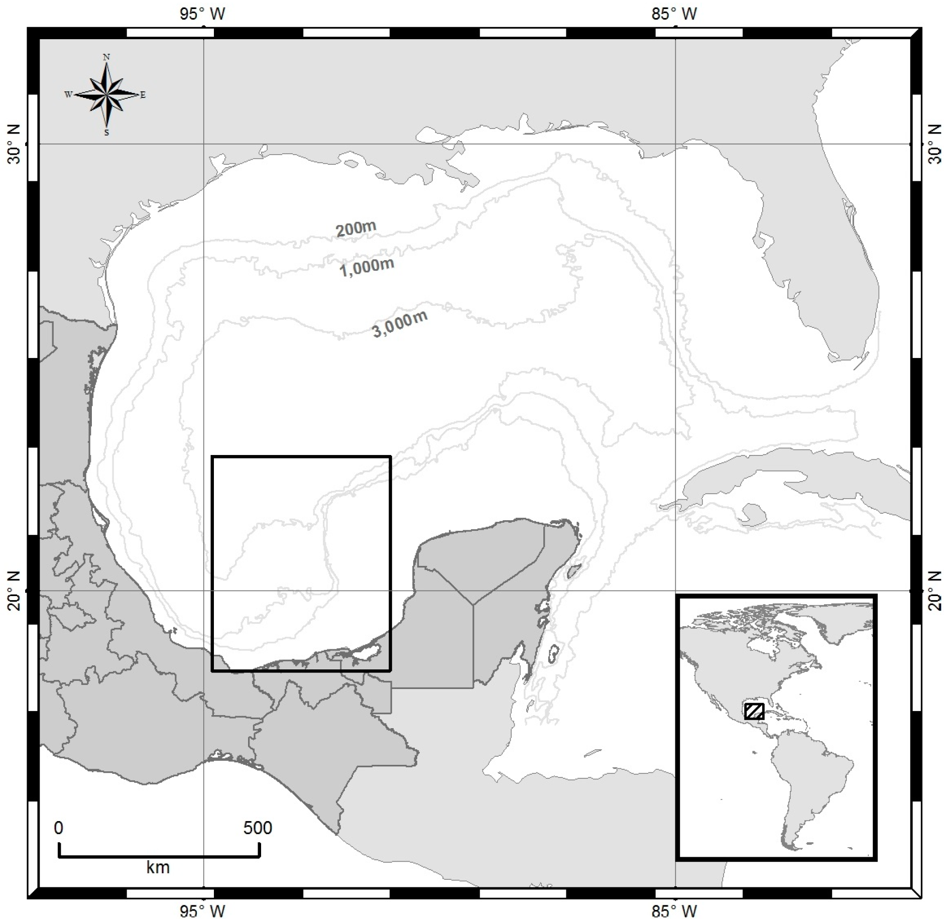
2. Dataset
3. Methods
3.1. Workable-Database Preparation
3.1.1. RADARSAT Re-Processing
3.1.2. New Slick-Feature Attributes
- 1st) Contextual Information: The Category attribute informs the oil slick type of each polygon: seeps or spills. Two other attributes provide the geographical location of the oil slick’s centroid: latitude (cLAT) and longitude (cLONG). A pair of satellite overpass attributes provides imaging time (SARtime) and observation date (SARdate).
- 2nd) SAR Scene Descriptors: The satellite scene is described by the imaging configuration (i.e., beam mode: Bmode) and the incidence angle (INC.ang). Regarding the latter, different basic statistical measures are also calculated, as shown when the 4th Attribute Type (i.e., SAR backscatter signature) are introduced.
- 3rd) Size Information: From the two basic morphological features originally present in the CBOS-Data, i.e., area (Area) and perimeter (Per), seven ratios are derived to describe the oil slicks’ geometry, shape, and dimension (Table 2). The first is the area to perimeter ratio (AtoP). Fiscella et al. [17] suggest using the perimeter to area ratio (PtoA). Fiscella et al. [17] and Singha et al. [18] recommend using a dimensionless normalized perimeter to area ratio (PtoA.nor). While small PtoA.nor values are related to simple geometry, larger values come from oil slicks with more complex geometries [19]. A dimensionless complexity measure is given by [20]: COMPLEX.ind. In addition, Bentz et al. [21] uses another dimensionless descriptor to illustrate how compact (i.e., close to a circle) is a sea-surface feature: COMPACT.ind. Two other indices have been utilized by [22]: SHAPE.ind and FRACTAL.ind. While these indices yield values close to the unit for regular forms (i.e., circular or square, respectively), larger numbers represent form irregularity [23]. The total number of pixels inside each oil slick polygon (LEN) is also provided.
- 4th) SAR Backscatter Signature: All pixels within individual polygons are utilized to calculate the different basic statistical measures experimentally used to characterize the oil slick SAR backscatter signature (Table 3). These are separately calculated for the twelve radiometric-calibrated image products (Table 1). As suggested by [18,21], an arithmetic mean (AVG) of all pixels of each oil slick is computed. Three other central tendency representations are also considered: median (MED), mode (MOD), and mid-mean (MDM). To analyze the SAR backscatter signature spread, six dispersion measures are considered: standard deviation (STD), coefficient of dispersion (COD), variance (VAR), total range (RNG), average absolute deviation (AAD), and median absolute deviation (MAD). The coefficient of variation (COV) evaluates the relative relationship between dispersion and central tendency, thus comparing the degree of variation of data with different units and different meanings. COV originally involves the ratio between STD and AVG, but herein other pair-values are also given (Table 3). Different authors recommend exploring COV, e.g., [18,24] refer to it as power-to-mean ratio, whereas [20] describe it as the oil slick’s homogeneity, and for [21] it depicts the oil slick’s heterogeneity. However, Miranda [25] emphasizes that oil slicks with different spatial structures (i.e., with completely different pixel configuration) can have identical average or median values and the same standard deviation. Minimum (MIN) and maximum (MAX) values of the pixels inside each polygon are also used as supplementary quantities.
3.1.3. Data Treatment Processes
- Log10 Transformation: Various non-linear transformations (e.g., square, cubic, or fourth root, as well as natural and base 10 logarithms) were tested to bring non-symmetric distributions to, or at least close to, a normal distribution pattern. Through the visual analyses of their histograms, Log10 had best results to stabilize the data, thus decreasing the effect of outliers and reducing skewness. The exception is FRACTAL.ind with its negative to positive range that was transformed as the cubic root.
- Negative Values Scaling: Because log functions cannot be applied to negative values, all pixels inside the oil slicks were inspected before such transformation. This mostly relates to the SAR Backscatter Signature (4th Attribute Type: Table 3), as the other Attribute Types all have positive values (except FRACTAL.ind). This specific Data Treatment Process consists of subtracting the minimum negative pixel value within the oil slick (PIXmin) from each pixel inside the oil slick (PIX) and adding one to it: PIXpos = [PIX − PIXmin + 1], where PIXpos is the new positive value. This simply adds two constants to each pixel, i.e., PIXmin and 1. The pixel with the minimum negative value becomes equal to 1, as PIX = PIXmin gives PIXpos = 1. Although this changes the values of the pixels inside some oil slicks, the relationship among pixel values within individual oil slicks is preserved [27,28].
- Ranging Standardization: While some quantitative attributes are dimensionless (e.g., dB), others have incompatible units. To compare the oil slick characteristics in the subsequent data mining exercise of our EDA, a common scale is recommended [29,30,31]. Of the various available methods, there is no dearth of standardization; however, Milligan and Cooper [32] advocated that Ranging could be more effective than other methods (e.g., z-score). The Ranging standardization, besides bounding the magnitude of the attributes between zero (0) and one (1), also equalizes the variability of the attributes to a common scale: Xranged = [X − Xmin]/[Xmax − Xmin], where Xranged is the new Ranged value, X is the actual attribute value for a particular oil slick, Xmin and Xmax are, respectively, the minimum and maximum values of this attribute among all oil slicks [27]. For instance, if taking the SIG.amp.AVG value of one oil slick: subtract the minimum AVG for this radiometric-calibrated image product among all 4916 oil slicks, then the result is divided by the maximum AVG of all 4916 oil slicks minus the minimum AVG of all 4916 oil slicks. The Xranged variables assume non-negative values, and only one oil slick has Xranged = 0 and another one Xranged = 1, respectively when X = Xmin and when X = Xmax.
- Dummy Variables: Certain qualitative attributes, such as string variables (Category and Bmode) and spatio-temporal variables (SARtime, SARdate, cLAT, and cLONG), have been converted to a specific indicator type: “dummy variable” [30]. For convenience, these have values of one (1) or zero (0), thus referring to its presence (Yes) or absence (No), respectively. These types of binary-coded variables attempt to decompose complex variabilities (or hidden knowledge) into more useful information.
3.2. Multivariate Data Analysis
3.2.1. Attribute Selection Methods
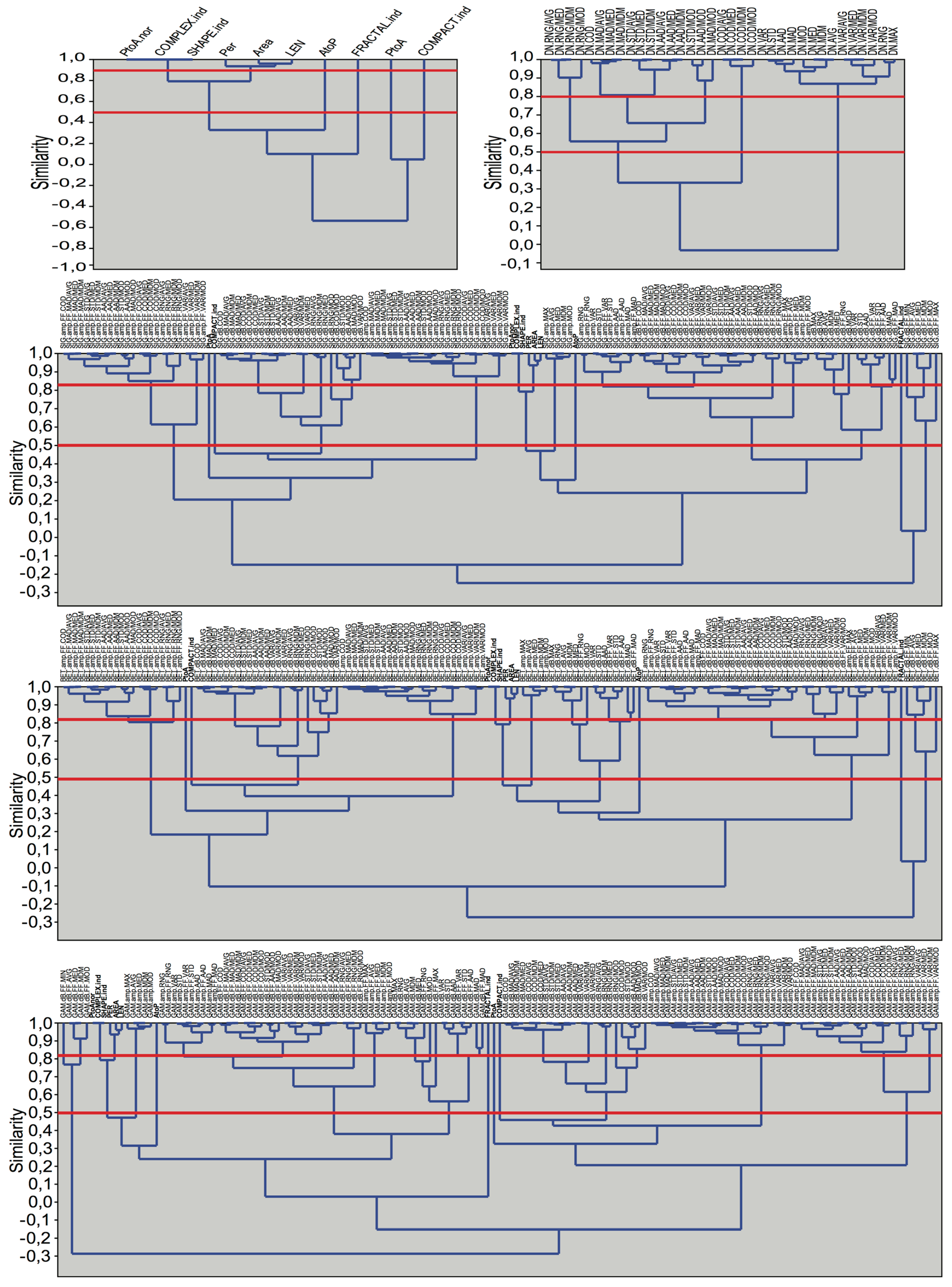
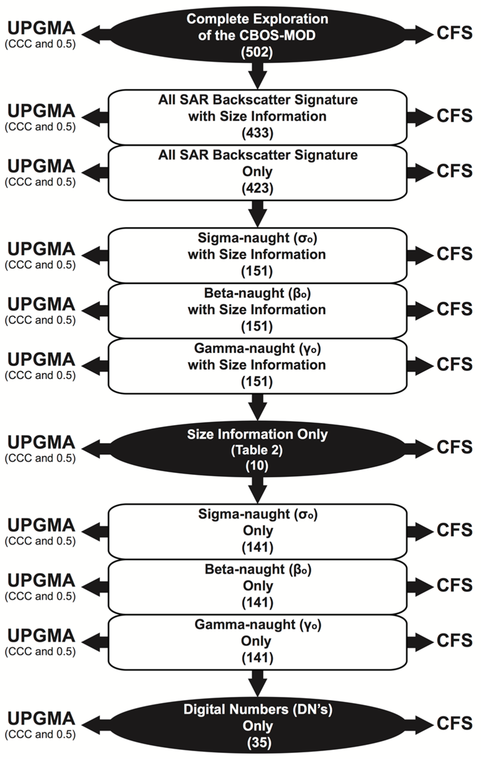
- Unweighted Pair Group Method with Arithmetic Mean (UPGMA): The resemblance between variables is revealed on a semi-automatic manner, in which an equally weighted pair wise group relationship among variables is used to form groups [27]. A variable is attributed to a group that has a larger similarity measure, i.e., Pearson’s r correlation coefficient, with all other variables of that same group [30,31]. A free scientific data analysis software package (PAST: PAleontological STatistics version 2.17c; Oslo, Norway) was utilized [33]. Rooted-tree dendrograms (i.e., diagrams of relationships) with a bootstrapping of 100 replicates help to find hierarchical relationships (i.e., affinity) among variables. Due to the large subjectivity while using dendrograms to form groups, two user-defined thresholds are explored [34]. Their choice aims to guarantee repeatability, as different thresholds give different groups of variables. The first threshold subjectively uses the Cophenetic Correlation Coefficient (CCC) that is automatically calculated in PAST to specify the clusters; its value varies depending upon dataset [35,36]. The second threshold is simply the fixed similarity value of 0.5. These two thresholds are used to draw horizontal lines (i.e., phenon lines) across the dendrograms, and when such lines cross a branch, a group is formed; from each group of similar variables only one variable is selected [37,38]. The Attribute Selection occurs twice for each UPGMA implementation, one for each phenon line, i.e., CCC and 0.5. This variable selection gives preference to an arbitrary user-defined strategy based on the simplicity of their meanings and on their calculation form, in which simple variables are preferred over complicated ones—e.g., basic variables in lieu of ratios (e.g., Area versus AtoP), C1 (amplitude) compared with C2 (dB), SAR backscatter signature without rather than with Frost filter, and central tendency is preferable to dispersion metrics. The variables choice follows the order presented on Table 1, Table 2 and Table 3.
- Correlation-Based Feature Selection (CFS): The CFS Attribute Selection is a fully automated process based on a heuristic variable selection strategy [39,40]. The “Merit” of various groups of selected variables is evaluated to select attributes with low inter-correlation but highly correlated to the categories being distinguished [41,42]. In essence, a Merit is calculated as a measure of the usefulness of the selected best possible group of attributes. A scientific machine learning open source package (WEKA: Waikato Environment for Knowledge Analysis version 3.6.12; Waikato, New Zealand) was utilized. The user specifies an evaluation function and a search algorithm [43,44,45]. The former is the method by which the groups of attributes are evaluated (Backward Sequential Selection: CfsSubsetEval), and the latter improves the evaluation function (best-first searching strategy: BestFirst).
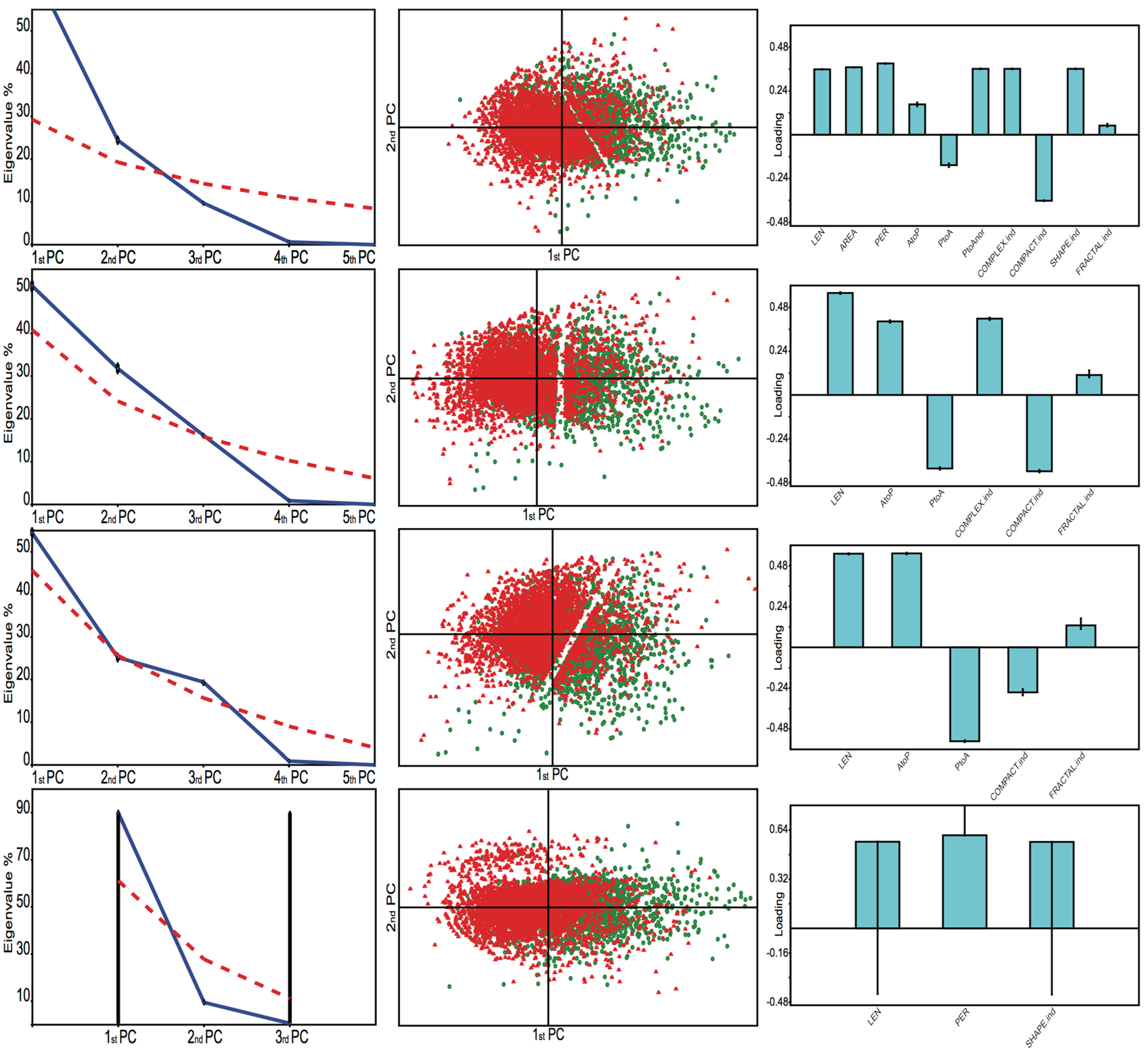
3.2.2. Principal Components Analysis (PCA)
3.2.3. Correlation Matrix
3.2.4. Discriminant Function
3.2.5. Oil Slick Classification Algorithm
4. Results
4.1. Workable-Database Preparation
4.1.1. RADARSAT Re-Processing
4.1.2. New Slick-Feature Attributes
4.1.3. Data Treatment Processes
4.2. Multivariate Data Analysis
4.2.1. Attribute Selection Methods
4.2.2. Principal Components Analysis (PCA)
4.2.3. Correlation Matrix
4.2.4. Discriminant Function
4.2.5. Oil Slick Classification Algorithm
5. Discussion
- Information from the area surrounding the oil slicks, i.e., background oil-free surface, could come into play, e.g., damping ratio [66];
- Information about radar beam incidence angles and environmental configurations (e.g., wind conditions) could add knowledge to the differentiation process;
- The number of individual non-contiguous parts forming oil slick polygons could be explored along with other contextual properties, such as the distance between centroid and the shoreline or the distance from a possible point source, i.e., oil rig complex or oil seep site location on the sea surface [21];
- Other methods instead of Ranging Standardization could be applied during the Data Treatment Process, e.g., z-score [30];
- As an alternative to the proposed automatic Attribute Selection Methods to select groups and variables, visual analyses of the UPGMA dendrograms could be instituted, or even other custom methods, e.g., Ward’s [30];
- Clustering Analyses (e.g., K-means) could also reveal natural groupings among oil slicks, thus supporting the oil slick type differentiation process.
6. Conclusions
- Yes. The seeped oil has SAR backscatter signatures (i.e., σo, βo, and γo) distinctive enough to distinguish it from anthropogenically-spilled oil;
- Yes. The Size Information (i.e., attributes describing the geometry, shape, and dimension of the oil slicks) can be used to distinguish seeps from spills, and in fact, the sole and simple use of area and perimeter can also distinguish natural from man-made oil slicks with an overall accuracy of about 70%; and;
- The synergistic combination of various oil slick characteristics leads to systems capable of distinguishing between seeped and spilled oil, in which different combinations of variables promote similar differentiation; however, the one leading to the most effective classification is represented by the sole and simple use of area and perimeter (70%), whereas the one with the worst capabilities have variables expressed in Digital Numbers (DNs).
Acknowledgments
Conflicts of Interest
References
- Jackson, C.R.; Apel, J.R. Synthetic Aperture Radar Marine User’s Manual; NOAA/NESDIS; Office of Research and Applications: Washington, DC, USA, 2004. Available online: http://www.sarusersmanual.com (accessed on 13 November 2017).
- Chan, Y.K.; Koo, V.C. An introduction to synthetic aperture radar (SAR). Prog. Electromagn. Res. B 2008, 2, 27–60. [Google Scholar] [CrossRef]
- Espedal, H.A.; Johannessen, O.M.; Knulst, J. Satellite detection of natural films on the ocean surface. Geophys. Res. Lett. 1996, 23, 3151–3154. [Google Scholar] [CrossRef]
- Johannessen, O.M.; Espedal, H.A.; Jenkins, A.J.; Knulst, J. SAR surveillance of ocean surface slicks. In Proceedings of the Second ERS Application Workshop, London, UK, 6–8 December 1995; pp. 187–192. [Google Scholar]
- Topouzelis, K. Oil spill detection by SAR Images: Dark formation detection, feature extraction and classification algorithms. Sensors 2008, 8, 6642–6659. [Google Scholar] [CrossRef] [PubMed] [Green Version]
- Mchugh, S.L. Satellite Synthetic Aperture radar in the Prosecution of Illegal Oil Discharges. Master’s Thesis, Memorial University of Newfoundland, St. John’s, NL, Canada, 2009; p. 122. [Google Scholar]
- Mano, M.F.; Beisl, C.H.; Siqueira, C.Y.S.; Pereira, J.S. Evaluation of remote technologies applied to natural seep mapping and their impact in oil exploration. In Proceedings of the Rio Oil & Gas Expo and Conference, Rio de Janeiro, Brazil, 15–18 September 2014; p. 7. [Google Scholar]
- Carvalho, G.A. Multivariate data Analysis of Satellite-Derived Measurements to Distinguish Natural from Man-Made Oil Slicks on the Sea Surface of Campeche Bay (Mexico). Ph.D. Dissertation, Universidade Federal do Rio de Janeiro (UFRJ), COPPE, Rio de Janeiro, Brazil, 2015; p. 285. Available online: http://www.coc.ufrj.br/index.php?option=com_content&view=article&id=5354:gustavo-de-araujo-carvalho (accessed on 13 November 2017).
- Carvalho, G.A.; Minnett, P.J.; Miranda, F.P.; Landau, L.; Moreira, F. The use of a RADARSAT-derived long-term dataset to investigate the sea surface expressions of human-related oil spills and naturally-occurring oil seeps in Campeche Bay, Gulf of Mexico. Can. J. Remote Sens. 2016, 42, 307–321. [Google Scholar] [CrossRef]
- Carvalho, G.A.; Landau, L.; Miranda, F.P.; Minnett, P.; Moreira, F.; Beisl, C. The use of RADARSAT-derived information to investigate oil slick occurrence in Campeche Bay, Gulf of Mexico. In Proceedings of the XVII Brazilian Remote Sensing Symposium (SBSR), INPE, João Pessoa, Brazil, 25–29 April 2015; pp. 1184–1191. Available online: http://www.dsr.inpe.br/sbsr2015/files/p0217.pdf (accessed on 13 November 2017).
- Freeman, A. Radiometric calibration of SAR image data. In Proceedings of the XVII Congress for Photogrammetry and Remote Sensing (ISPRS), Washington, DC, USA, 2–14 August 1992; pp. 212–222. [Google Scholar]
- El-darymli, K.; Mcguire, P.; Gill, E.; Power, D.; Moloney, C. Understanding the significance of radiometric calibration for synthetic aperture radar imagery. In Proceedings of the IEEE 27th Canadian Conference on Electrical and Computer Engineering (CCECE), Toronto, ON, Canada, 4–7 May 2014; p. 6. [Google Scholar] [CrossRef]
- ESA (European Space Agency). 2014. Available online: http://earth.eo.esa.int/polsarpro/ (accessed on 1 August 2016).
- Thakur, P.K. SAR data processing to extract backscatter response from various features. In Proceedings of the Symposium Tutorials on Polarimetric SAR Data Processing and Applications, International Society for Photogrametry and Remote Sensing (ISPRS), Hyderabad, India, 9–12 December 2014. [Google Scholar]
- ASF (Alaska Satellite Facility). MapReady User Manual Remote Sensing Tool Kit, Engineering Group. 2015. Available online: https://media.asf.alaska.edu/uploads/pdf/mapready_manual_3.1.22.pdf (accessed on 13 November 2017).
- Frost, V.S.; Stiles, J.A.; Shanmugan, K.S.; Holtzman, J.C. A model for radar images and its application to adaptive digital filtering of multiplicative noise. IEEE Trans. Pattern Anal. Mach. Intell. 1982, 4, 157–166. [Google Scholar] [CrossRef] [PubMed]
- Fiscella, B.; Giancaspro, A.; Nirchio, F.; Pavese, P.; Trivero, P. Oil spill monitoring in the Mediterranean Sea using ERS SAR data. In Proceedings of the Envisat Symposium, ESA, Göteborg, Sweden, 16–20 October 2010; p. 9. [Google Scholar]
- Singha, S.; Bellerby, T.J.; Trieschmann, O. Satellite Oil Spill Detection Using Artificial Neural Networks. IEEE J. Sel. Top. Appl. Earth Obs. Remote Sens. 2013, 6, 9. [Google Scholar] [CrossRef]
- Calabresi, G.; Del Frate, F.; Lichtenegger, I.; Petrocchi, A.; Trivero, P. Neural networks for the oil spill detection using ERS–SAR data. In Proceedings of the IEEE International Geoscience and Remote Sensing Symposium (IGARSS ’99), Hamburg, Germany, 28 June–2 July 1999; pp. 215–217. [Google Scholar] [CrossRef]
- Solberg, A.H.S.; Storvik, G.; Solberg, R.; Volden, E. Automatic detection of oil spills in ERS SAR images. IEEE Trans. Geosci. Remote Sens. 1999, 37, 1916–1924. [Google Scholar] [CrossRef]
- Bentz, C.M. Reconhecimento Automático de Eventos Ambientais Costeiros e Oceânicos em Imagens de Radares Orbitais. Ph.D. Dissertation, Universidade Federal do Rio de Janeiro (UFRJ), COPPE, Rio de Janeiro, Brazil, 2006; p. 115. [Google Scholar]
- Pisano, A. Development of Oil Spill Detection Techniques for Satellite Optical Sensors and Their Application to Monitor Oil Spill Discharge in the Mediterranean Sea. Ph.D. Dissertation, Università di Bologna, Bologna, Italy, 2011; p. 146. [Google Scholar]
- McgarigaL, K.; Marks, B.J. FRAGSTATS: Spatial Pattern Analysis Program for Quantifying Landscape Structure. USDA For. Serv. Gen. Tech. Rep. PNW-351. 1994, p. 134. Available online: http://www.umass.edu/landeco/pubs/mcgarigal.marks.1995.pdf (accessed on 13 November 2017).
- Solberg, A.H.S.; Volden, E. Incorporation of prior knowledge in automatic classification of oil spills in ERS SAR images. In Proceedings of the IEEE International Geoscience and Remote Sensing Symposium (IGARSS ’97), Singapore, 3–8 August 1997; pp. 157–159. [Google Scholar]
- Miranda, F.P. Reconnaissance Geologic Mapping of a Heavily-Forested Shield Area (Guiana Shield, Northwestern Brazil). Ph.D. Dissertation, University of Nevada, Reno, NV, USA, 1990; p. 176. [Google Scholar]
- Fiscella, B.; Giancaspro, A.; Nirchio, F.; Pavese, P.; Trivero, P. Oil spill detection using marine SAR images. Int. J. Remote Sens. 2000, 21, 3561–3566. [Google Scholar] [CrossRef]
- Sneath, P.H.A.; SokaL, R.R. Numerical Taxonomy—The principles and Practice of Numerical Classification; W.H. Freeman and Company: San Francisco, CA, USA, 2017; p. 573. ISBN 0-7167-0697-0. [Google Scholar]
- Lane, D.M.; Scott, D.; Hebl, M.; Guerra, R.; Osherson, D.; Ziemer, H. Introduction to Statistics. 2015. Available online: http://onlinestatbook.com/Online_Statistics_Education.pdf (accessed on 13 November 2017).
- Moita Neto, J.M.; Moita, G.C. Uma introdução à análise exploratória de dados multivariados. Quím. Nova 1998, 21, 467–469. [Google Scholar] [CrossRef]
- Legendre, P.; Legendre, L. Developments in Environmental Modelling. In Numerical Ecology, Third ed.; Elsevier Science B.V.: Amsterdam, The Netherlands, 2012; p. 990. ISBN 978-0444538680. [Google Scholar]
- Valentin, J.L. Ecologia Numérica–Uma Introdução à Análise Multivariada de Dados Ecológicos, Second ed.; Editora Interciência: Rio de Janeiro, Brazil, 2012; 153p, ISBN 978-85-7193-230-2. [Google Scholar]
- Milligan, G.W.; Cooper, M.C. A study of standardization of variables in cluster analysis. J. Classif. 1988, 5, 181–204. [Google Scholar] [CrossRef]
- Hammer, Ø.; Harper, D.A.T.; Ryan, P.D. PAST: PAleontological STatistics software package for education and data analysis. Palaeontol. Electron. 2001, 4, 9. Available online: http://palaeo-electronica.org/2001_1/past/issue1_01.htm (accessed on 13 November 2017).
- Kelley, L.A.; Gardner, S.P.; Sutcliffe, M.J. An automated approach for clustering an ensemble of NMR-derived protein structures into conformationally related subfamilies. Protein Eng. Des. Sel. 1996, 9, 1063–1065. [Google Scholar] [CrossRef]
- Farris, J.S. On the cophenetic correlation coefficient. Syst. Biol. 1969, 18, 279–285. [Google Scholar] [CrossRef]
- Saraçli, S.; Dogan, N.; Dogan, I. Comparison of hierarchical cluster analysis methods by cophenetic correlation. J. Inequal. Appl. 2013, 2013, 203. [Google Scholar] [CrossRef]
- Sokal, R.R.; Rohlf, F.J. The Comparison of dendrograms by objective methods. Taxon 1962, 11, 33–40. [Google Scholar] [CrossRef]
- NCSS (Number Cruncher Statistical System). Hierarchical Clustering and Dendrograms. NCSS Statistical Software. 2015. Chapter 445. p. 15. Available online: http://ncss.wpengine.netdna-cdn.com/wp-content/themes/ncss/pdf/Procedures/NCSS/Hierarchical_Clustering-Dendrograms.pdf (accessed on 13 November 2017).
- Hall, M.A.; Smith, L.A. Feature subset selection: a correlation based filter approach. In Proceedings of the Fourth International Conference on Neural Information and Intelligent Information Systems, Dunedin, New Zealand, 24–28 November 1997; pp. 855–858. [Google Scholar]
- Hall, M.A.; Smith, L.A. Feature selection for machine learning: comparing a correlation-based filter approach to the wrapper. In Proceedings of the 12th International FLAIRS Conference, Orlando, FL, USA, 1–5 May 1999. [Google Scholar]
- Hall, M.A. Correlation-Based Feature Selection for Machine Learning. Ph.D. Dissertation, The University of Waikato, Department of Computer Science, Hamilton, New Zealand, 1999; p. 178. [Google Scholar]
- Bouckaert, R.R.; Frank, E.; Hall, M.; Kirkby, R.; Reutemann, P.; Seewald, A.; Scuse, D. WEKA Manual for Version 3–6-0; The University of Waikato: Hamilton, New Zealand, 2008; p. 212. Available online: http://citeseerx.ist.psu.edu/viewdoc/summary?doi=10.1.1.153.9743 (accessed on 13 November 2017).
- Aha, D.W.; Bankert, R.L. Feature selection for case-based classification of cloud types: An empirical comparison. In Case-Based Reasoning: Papers From the 1994 Workshop (Technical Report WS-94–01); Advancement of Artificial Intelligence (AAAI): Menlo Park, CA, USA, 1994; pp. 106–112. Available online: https://www.aaai.org/Papers/Workshops/1994/WS-94-01/WS94-01-019.pdf (accessed on 13 November 2017).
- Tetko, I.; Baskin, I.; Varnek, A. Tutorial on Machine Learning, Part 2: Descriptor Selection Bias. 2008. Available online: http://infochim.u-strasbg.fr/CS3/program/Tutorials/Tutorial2b.pdf (accessed on 13 November 2017).
- Wilt, C.; Thayer, J.; Ruml, W.A. Comparison of Greedy Search Algorithms. In Proceedings of the Third Annual Symposium on Combinatorial Search (SoCS-10), Atlanta, GA, USA, 8–10 July 2010; pp. 129–136. [Google Scholar]
- Thompson, A.A.; McLeod, I.H. The RADARSAT-2 SAR processor. Can. J. Remote Sens. 2004, 30, 336–344. [Google Scholar] [CrossRef]
- Peres-Neto, P.R.; Jackson, D.A.; Somers, K.M. Giving meaningful interpretation to ordination axes: Assessing loading significance in principal component analysis. Ecology 2003, 84, 2347–2363. [Google Scholar] [CrossRef]
- Peres-Neto, P.R.; Jackson, D.A.; Somers, K.M. How many principal components? Stopping rules for determining the number of non-trivial axes revisited. Comput. Stat. Data Anal. 2005, 49, 974–997. [Google Scholar] [CrossRef]
- Hair, J.F.; Anserson, R.E.; Tatham, R.L.; Black, W.C. Multivariate Data Analysis. In Análise Multivariada de Dados, Fifth ed.; Sant’Anna, A.S., Chaves Neto, A., Eds.; Bookman: Porto Alegre, RS, Brazil, 2005; ISBN 0-13-014406-7. [Google Scholar]
- Cattell, R.B. The Scree Test For The Number of Factors. Multivar. Behav. Res. 1966, 1, 245–276. [Google Scholar] [CrossRef] [PubMed]
- Jackson, D.A. Stopping Rules in Principal Components Analysis: A Comparison of Heuristical and Statistical Approaches. Ecology 1993, 74, 2204–2214. [Google Scholar] [CrossRef]
- Hammer, Ø. PAST: Multivariate Statistics. 2015. Available online: http://folk.uio.no/ohammer/past/multivar.html (accessed on 13 November 2017).
- Kaiser, H.F. A note on Guttman’s lower bound for the number of common factors. Br. J. Stat. Psychol. 1961, 14, 2. [Google Scholar] [CrossRef]
- Maimon, O.; Rokach, L. Data Mining and Knowledge Discovery Handbook, Second ed.; Springer Science: New York, NY, USA, 2010; p. 1285. [Google Scholar] [CrossRef]
- Carvalho, G.A.; Minnett, P.J.; Fleming, L.E.; Banzon, V.F.; Baringer, W. Satellite remote sensing of harmful algal blooms: A new multi-algorithm method for detecting the Florida Red Tide (Karenia brevis). Harmful Algae 2010, 9, 440–448. Available online: https://www.ncbi.nlm.nih.gov/pubmed/21037979 (accessed on 13 November 2017). [CrossRef] [PubMed]
- Carvalho, G.A.; Minnett, P.J.; Banzon, V.F.; Baringer, W.; Heil, C.A. Long-term evaluation of three satellite ocean color algorithms for identifying harmful algal blooms (Karenia brevis) along the west coast of Florida: A matchup assessment. Remote Sens. Environ. 2011, 115, 18. Available online: http://www.ncbi.nlm.nih.gov/pubmed/22180667 (accessed on 13 November 2017). [CrossRef] [PubMed]
- Congalton, R.G. A review of assessing the accuracy of classifications of remotely sensed data. Remote Sens. Environ. 1991, 37, 35–46. [Google Scholar] [CrossRef]
- Nussmeier, N.A.; Miao, Y.; Roach, G.W.; Wolman, R.L.; Mora-Mangano, C.; Fox, M.; Szekely, A.; Tommasino, C.; Schwann, N.M.; Mangano, D.T. Predictive value of the National Institutes of Health Stroke Scale and the Mini-Mental State Examination for neurologic outcome after coronary artery bypass graft surgery. J. Thorac. Cardiovasc. Surg. 2010, 139, 901–912. [Google Scholar] [CrossRef] [PubMed]
- Lee, M.-J.; Yun, M.J.; Park, M.-S.; Cha, S.H.; Kim, M.-J.; Lee, J.D.; Kim, K.W. Paraaortic lymph node metastasis in patients with intraabdominal malignancies: CT vs PET. World J. Gastroenterol. 2009, 15, 4434–4438. [Google Scholar] [CrossRef] [PubMed]
- Carvalho, G.A. The Use of Satellite-Based Ocean Color Measurements for Detecting the Florida Red Tide (Karenia brevis). Ph.D. Thesis, University of Miami (UM/RSMAS/MPO), Miami, FL, USA, 2008; p. 156. Available online: http://scholarlyrepository.miami.edu/oa_theses/116/ (accessed on 13 November 2017).
- Alberg, A.J.; Park, J.W.; Hager, B.W.; Brock, M.V.; Diener-West, M. The use of “overall accuracy” to evaluate the validity of screening or diagnostic tests. J. Gen. Intern. Med. 2004, 19, 460–465. [Google Scholar] [CrossRef] [PubMed]
- Theriault, C.; Scheibling, R.; Hatcher, B.; Jones, W. Mapping the distribution of an invasive marine alga (Codium fragile spp. tomentosoides) in optically shallow coastal waters using the compact airborne spectrographic imager (CASI). Can. J. Remote Sens. 2006, 32, 315–329. [Google Scholar] [CrossRef]
- Espedal, H.A.; Johannessen, O.M. Cover: Detection of oil spills near offshore installations using synthetic aperture radar (SAR). Int. J. Remote Sens. 2000, 21, 2141–2144. [Google Scholar] [CrossRef]
- Espedal, H.A. Detection of oil spill and natural film in the marine environment by spaceborne synthetic aperture radar. Ph.D. Dissertation, Department of Physics, University of Bergen and Nansen Environmental and Remote Sensing Center (NERSC), Bergen, Norway, 1998; p. 200. [Google Scholar]
- Espedal, H. Detection of oil spill and natural film in the marine environment by spaceborne SAR. In Proceedings of the IEEE International Geoscience and Remote Sensing Symposium (IGARSS ’99), Hamburg, Germany, 28 June–2 July 1999; pp. 1478–1480. [Google Scholar] [CrossRef]
- Holt, B. SAR imaging of the ocean surface. In Synthetic Aperture Radar Marine User’s Manual; NOAA/NESDIS; Office of Research and Applications: Washington, DC, USA, 2004; Chapter 2; pp. 25–79. Available online: http://www.sarusersmanual.com (accessed on 13 November 2017).
- Klinkenberg, B. A review of methods used to determine the fractal dimension of linear features. Math. Geol. 1994, 26, 23–46. [Google Scholar] [CrossRef]
- Bevilacqua, L.; Barros, M.M.; Galeão, A.C.R.N. Geometry, dynamics and fractals. J. Br. Soc. Mech. Sci. Eng. 2008, 30, 11–21. [Google Scholar] [CrossRef]
- Ledesma, R.D.; Valero-Mora, P. Determining the number of factors to retain in EFA: an easy-to-use computer program for carrying out Parallel Analysis. Pract. Assess. Res Eval. 2007, 12, 11. [Google Scholar]
- Garcia-Pineda, O.; MacDonald, I.; Zimmer, B. Synthetic aperture radar image processing using the Supervised Textural-Neural Network Classification Algorithm. In Proceedings of the IEEE International Geoscience and Remote Sensing Symposium (IGARSS ’08), Boston, MA, USA, 8–11 July 2008; pp. IV:1265–IV:1268. [Google Scholar] [CrossRef]
- Garcia-Pineda, O.; MacDonald, I.; Zimmer, B.; Shedd, B.; Roberts, H. Remote-sensing evaluation of geophysical anomaly sites in the outer continental slope, northern Gulf of Mexico. Deep Sea Res. Part II: Top. Stud. Oceanogr. 2010, 57, 1859–1869. [Google Scholar] [CrossRef]
- Garcia-Pineda, O.; Zimmer, B.; Howard, M.; Pichel, W.; Li, X.; MacDonald, I.R. Using SAR images to delineate ocean oil slicks with a texture-classifying neural network algorithm (TCNNA). Can. J. Remote Sens. 2009, 35, 411–421. [Google Scholar] [CrossRef]
- Mityagina, M.; Lavrova, O. Satellite Survey of Inner Seas: Oil Pollution in the Black and Caspian Seas. Remote Sens. 2016, 8, 875. [Google Scholar] [CrossRef]
- Song, D.; Ding, Y.; Li, X.; Zhang, B.; Xu, M. Ocean Oil Spill Classification with RADARSAT-2 SAR Based on an Optimized Wavelet Neural Network. Remote Sens. 2017, 9, 799. [Google Scholar] [CrossRef]
- Migliaccio, M.; Nunziata, F.; Buono, A. SAR polarimetry for sea oil slick observation. Int. J. Remote Sen. 2015, 36, 3243–3273. [Google Scholar] [CrossRef]


| Image Products | Frost Filter | σo | βo | γo |
|---|---|---|---|---|
| C1 in Amplitude | Without | SIG.amp | BET.amp | GAM.amp |
| With | SIG.amp.FF | BET.amp.FF | GAM.amp.FF | |
| C2 in dB | Without | SIG.dB | BET.dB | GAM.dB |
| With | SIG.dB.FF | BET.dB.FF | GAM.dB.FF | |
| Incience angle (INC.ang) | ||||
| 1st Attribute Type: Contextual Information § | ||||
| 1 | Category | Spill or Seep | Oil Slick Type * | |
| 2 | Class | See [8] | ||
| 3 | cLAT | Latitude (° N) | Spatial Location | |
| 4 | cLONG | Longitude (° W) | ||
| 5 | SARtime | Overpass Time | Temporal Location | |
| 6 | SARdate | Overpass Date | ||
| 2nd Attribute Type: SAR Scene Descriptor | ||||
| 1 | Bmode § * | Beam mode | ||
| 2–37 ** | INC.ang | Incidence angle of the radar beam | ||
| 3rd Attribute Type: Size Information (Geometry, Shape, and Dimension) | ||||
| 1 | LEN | Number of pixels inside the oil slick polygon. | ||
| 2 | Area § | km2 | ||
| 3 | Per § | km | Perimeter | |
| 4 | AtoP | km | Area to Per ratio | Area/Per |
| 5 | PtoA | km−1 | Per to Area ratio | Per/Area |
| 6 | PtoA.nor | * | Normalized PtoA | Per/[(2 × (Pi × Area))^(1/2)] |
| 7 | COMPLEX.ind | * | Complexity Index | (Per2)/Area |
| 8 | COMPACT.ind | * | Compact Index | (4 × Pi × Area)/(Per2) |
| 9 | SHAPE.ind | km−1 | Shape Index | [0.25 × Per]/[Area^(1/2)] |
| 10 | FRACTAL.ind | * | Fractal Index | [2 × ln(0.25 × Per)]/[ln(Area)] |
| 4th Attribute Type: SAR Backscatter Signature | 36 × 12 = 432 | |||
|---|---|---|---|---|
| Basic Statistical Measures | 12 × 12 = 144 | |||
| 1 | 1–12 | AVG | Average | Central Tendency (4) |
| 2 | 13–24 | MED | Median | |
| 3 | 25–36 | MOD | Mode | |
| 4 | 37–48 | MDM * | Mid-Mean | |
| 5 | 49–60 | STD | Standard Deviation | Dispersion (6) |
| 6 | 61–72 | COD ** | Coefficient of Dispersion | |
| 7 | 73–84 | VAR | Variance | |
| 8 | 85–96 | RNG | Total Range | |
| 9 | 97–108 | AAD *** | Average Absolute Deviation | |
| 10 | 109–120 | MAD **** | Median Absolute Deviation | |
| 11 | 121–132 | MIN § | Minimum | |
| 12 | 133–144 | MAX | Maximum | |
| COV = Coefficient of Variation | 24 × 12 = 288 | |||
| 13 | 145–156 | COV.STD/AVG ¥ | 1st combined COV set (STD divided by Central Tendency) | |
| 14 | 157–168 | COV.STD/MED | ||
| 15 | 169–180 | COV.STDMOD | ||
| 16 | 181–192 | COV.STD/MDM | ||
| 17 | 192–204 | COV.COD/AVG | 2nd combined COV set (COD divided by Central Tendency) | |
| 18 | 205–216 | COV.COD/MED | ||
| 19 | 217–228 | COV.COD/MOD | ||
| 20 | 229–240 | COV.COD/MDM | ||
| 21 | 241–252 | COV.VAR/AVG | 3rd combined COV set (VAR divided by Central Tendency) | |
| 22 | 253–264 | COV.VAR/MED | ||
| 23 | 265–276 | COV.VAR/MOD | ||
| 24 | 277–288 | COV.VAR/MDM | ||
| 25 | 289–300 | COV.RNG/AVG | 4th combined COV set (RNG divided by Central Tendency) | |
| 26 | 301–312 | COV.RNG/MED | ||
| 27 | 313–324 | COV.RNG/MOD | ||
| 28 | 325–336 | COV.RNG/MDM | ||
| 29 | 337–348 | COV.AAD/AVG | 5th combined COV set (AAD divided by Central Tendency) | |
| 30 | 349–360 | COV.AAD/MED | ||
| 31 | 361–372 | COV.AAD/MOD | ||
| 32 | 373–384 | COV.AAD/MDM | ||
| 33 | 385–396 | COV.MAD/AVG | 6th combined COV set (MAD divided by Central Tendency) | |
| 34 | 397–408 | COV.MAD/MED | ||
| 35 | 409–420 | COV.MAD/MOD | ||
| 36 | 421–432 | COV.MAD/MDM | ||
| § | Algorithm Outcome Seeps | Algorithm Outcome Spills | § | Algorithm Outcome Seeps | Algorithm Outcome Spills | ||||
| Actual Seeps | GOOD Seeps | BAD Seeps | All Actual Seeps | Actual Seeps | A | B | A + B | ||
| Actual Spills | BAD Spills | GOOD Spills | All Actual Spills | Actual Spills | C | D | C + D | ||
| All Algorithm Seeps | All Algorithm Spills | All Actual Slicks | A+C | B+D | A + B + C + D | ||||
| Overall Accuracy | Overall Accuracy | ||||||||
| ¥ | Algorithm Outcome Seeps | Algorithm Outcome Spills | ¥ | Algorithm Outcome Seeps | Algorithm Outcome Spills | ||||
| Actual Seeps | Sensitivity | Actual Seeps | 100% | Actual Seeps | 100% | ||||
| Actual Spills | False Positive | Specificity | 100% | Actual Spills | 100% | ||||
| ¥ | Algorithm Outcome Seeps | Algorithm Outcome Spills | ¥ | Algorithm Outcome Seeps | Algorithm Outcome Spills | ||||
| Actual Seeps | Positive Predictive Value | Invert Neg Predictive Value | Actual Seeps | ||||||
| Actual Spills | Invert Pos Predictive Value | Negative Predictive Value | Actual Spills | ||||||
| 100% | 100% | 100% | 100% | ||||||
| PA/CE Q1) | How many known oil seep samples are correctly identified? Sensitivity: A, also given in percentage by (A × 100)/[A + B]. | ||||||||
| PA/CE Q2) | How many known oil spill samples are correctly identified? Specificity: D, also given in percentage by (D × 100)/[C + D]. | ||||||||
| PA/CE Q3) | How many known oil seep samples are misidentified? False Negative cases: B, also given in percentage by (B × 100)/[A + B]. Coupled with Sensitivity. | ||||||||
| PA/CE Q4) | How many known oil spill samples are misidentified? False Positive cases: C, also given in percentage by (C × 100)/[C + D]. Linked to Specificity. | ||||||||
| UA/OE Q1) | How many oil seeps identified by the Function are indeed known oil seeps? Positive Predictive Value: A, also given in percentage by (A × 100)/[A + C]. | ||||||||
| UA/OE Q2) | How many oil spills identified by the Function are indeed known oil spills? Negative Predictive Value: D, also given in percentage by (D × 100)/[B + D]. | ||||||||
| UA/OE Q3) | Of samples identified by the Function as oil seeps, how many are oil spills? Inverse of the Positive Predictive Value: C, also given in percentage by (C × 100)/[A + C]. | ||||||||
| UA/OE Q4) | Of samples identified by the Function as oil spills, how many are oil seeps? Inverse of the Negative Predictive Value: B, also given in percentage by (B × 100)/[B + D]. | ||||||||
| 11 Original Sets and 33 Optimal Subsets | 1) Values of | 2) Number of Variables: | 3) Number of Selected PC’s: | |||||||
|---|---|---|---|---|---|---|---|---|---|---|
| UPGMA (CCC) | CFS (Merit) | Original Sets | UPGMA | CFS | Original Sets | UPGMA | CFS | |||
| (CCC) | (0.5) | (CCC) | (0.5) | |||||||
| 1. Complete Exploration of the CBOS-MOD | 0.8175 | 1.000 | 502 | 59 | 46 | 15 # | 10 | 21 | 18 | § |
| 2. ❖ With Size Information | 0.8227 | 0.131 | 433 | † | † | 20 | 8 | † | † | 6 |
| 3. ❖ Only | 0.8253 | 0.103 | 423 | †† | †† | 36 | 7 | †† | †† | 6 |
| 4. σo with Size Information | 0.8262 | 0.127 | 151 | 26 | 12 | 26 | 6 | 7 | 3 | 7 |
| 5. βo with Size Information | 0.8031 | 0.129 | 151 | 25 | 12 | 15 | 6 | 7 | 3 | 5 |
| 6. γo with Size Information | 0.8240 | 0.126 | 151 | 26 | 12 | 19 | 6 | 7 | 3 | 5 |
| 7. Size Information only | 0.9143 | 0.112 | 10 | 6 | 5 | 3 | 2 | 2 | 2 | 2 ¥ |
| 8. Only σo | 0.8319 | 0.099 | 141 | 20 | 7 | 24 | 5 | 5 | 2 | 4 |
| 9. Only βo | 0.8130 | 0.099 | 141 | 19 | 7 | 21 | 5 | 4 | 2 | 5 |
| 10. Only γo | 0.8260 | 0.097 | 141 | 20 | 7 | 22 | 6 | 5 | 2 | 4 |
| 11. DNs only | 0.8020 | 0.059 | 35 | 5 | 3 | 11 | 2 | 2 | 2 | 2 |
| Only Size Information | |
|---|---|
| UPGMA Selected Attributes | |
| 1 | LEN |
| 2 | AtoP |
| 3 | PtoA |
| 4 | COMPACT.ind |
| 5 | COMPLEX.ind |
| 6 | FRACTAL.ind |
| CFS Selected Attributes | |
| 1 | LEN |
| 2 | PER |
| 3 | SHAPE |
| Only DNs | |
| UPGMA Selected Attributes | |
| 1 | DN.AVG |
| 2 | DN.COD |
| 3 | DN.STD/MOD |
| 4 | DN.COD/AVG |
| 5 | DN.RNG/AVG |
| CFS Selected Attributes | |
| 1 | DN.AVG |
| 2 | DN.MDM |
| 3 | DN.STD |
| 4 | DN.COD |
| 5 | DN.RNG |
| 6 | DN.COD/MOD |
| 7 | DN.RNG/AVG |
| 8 | DN.RNG/MED |
| 9 | DN.RNG/MOD |
| 10 | DN.RNG/MDM |
| 11 | DN.MAD/MED |
| Selection Method | UPGMA | CFS | CFS | |||||||
|---|---|---|---|---|---|---|---|---|---|---|
| Size Information | Without § | With | Without | |||||||
| Attribute Inventory | σo | βo | γo | σo | βo | γo | σo | βo | γo | |
| 1 | LEN | * | * | * | ||||||
| 2 | AREA | * | * | * | ||||||
| 3 | PER | * | * | * | ||||||
| 4 | AtoP | |||||||||
| 5 | PtoA | * | * | |||||||
| 6 | PtoAnor | * | ||||||||
| 7 | COMPACT.ind | * | * | * | ||||||
| 8 | COMPLEX.ind | * | * | |||||||
| 9 | SHAPE.ind | * | * | * | ||||||
| 10 | FRACTAL.ind | * | * | * | ||||||
| 1 | amp.AVG | ** | ** | ** | ||||||
| 2 | amp.MOD | * | * | * | ||||||
| 3 | amp.STD | ** | ** | ** | ||||||
| 4 | amp.COD | ** | ** | ** | * | * | * | * | * | * |
| 5 | amp.RNG | * | * | * | * | * | * | |||
| 6 | amp.MAX | * | * | * | ||||||
| 7 | amp.STD/MOD | * | ||||||||
| 8 | amp.STD/MDM | * | ||||||||
| 9 | amp.RNG/MED | * | * | |||||||
| 10 | amp.RNG/MOD | * | ||||||||
| 11 | amp.RNG/MDM | * | * | |||||||
| 12 | amp.MAD/AVG | * | ||||||||
| 13 | amp.FF.AVG | * | * | * | ||||||
| 14 | amp.FF.COD | ** | ** | ** | ||||||
| 15 | amp.FF.RNG | * | * | * | ||||||
| 16 | amp.FF.VAR/AVG | * | * | * | ||||||
| 17 | amp.FF.RNG/AVG | * | * | * | * | * | ||||
| 18 | amp.FF.RNG/MDM | * | ||||||||
| 19 | amp.FF.RNG/MOD | * | ||||||||
| 20 | dB.AVG | ** | ** | ** | ||||||
| 21 | dB.MED | * | * | * | * | |||||
| 22 | dB.MOD | * | * | * | ||||||
| 23 | dB.STD | * | * | * | * | * | * | * | * | |
| 24 | dB.COD | ** | ** | ** | * | * | * | * | * | |
| 25 | dB.MAD | * | * | * | * | * | * | * | * | |
| 26 | dB.STD/AVG | * | * | * | * | |||||
| 27 | dB.STD/MED | * | * | * | ||||||
| 28 | dB.STD/MOD | * | * | * | ||||||
| 29 | dB.VAR/AVG | * | * | * | * | * | * | * | * | |
| 30 | dB.VAR/MED | * | * | * | * | |||||
| 31 | dB.VAR/MOD | * | * | * | * | |||||
| 32 | dB.RNG/AVG | * | * | * | ||||||
| 33 | dB.RNG/MED | * | * | * | * | |||||
| 34 | dB.RNG/MOD | * | * | * | * | * | * | * | * | * |
| 35 | dB.FF.AVG | ** | ** | ** | ||||||
| 36 | dB.FF.COD | * | * | |||||||
| 37 | dB.FF.RNG | * | * | * | * | * | ||||
| 38 | dB.FF.MIN | * | * | |||||||
| 39 | dB.FF.MAX | * | * | * | ||||||
| 40 | dB.FF.MAD | * | * | * | * | * | * | |||
| 41 | dB.FF.COD/AVG | * | * | |||||||
| 42 | dB.FF.COD/MED | * | ||||||||
| 43 | dB.FF.VAR/AVG | * | ||||||||
| 44 | dB.FF.RNG/AVG | * | * | |||||||
| 45 | dB.FF.RNG/MOD | * | * | * | ||||||
| 46 | dB.FF.MAD/AVG | * | * | |||||||
| 47 | dB.FF.MAD/MOD | * | ||||||||
| 57 | Total (**) | 20 (7) | 19 (7) | 20 (7) | 26 | 15 | 19 | 24 | 21 | 22 |
| Hotelling’s t2 Values | Original Sets | UPGMA (CCC) | UPGMA (0.5) | CFS | |
|---|---|---|---|---|---|
| Complete Exploration | 17,056.0 | 89,403.0 | 94,086.0 | § | |
| All SAR Backscatter Signature * with Size Information | 1065.5 | † | † | 1044.5 | |
| All SAR Backscatter Signature * only | 598.9 | †† | †† | 632.4 | |
| σo | with Size Information | 891.0 | 1123.5 | 769.8 | 1065.8 |
| βo | with Size Information | 908.7 | 1099.5 | 722.3 | 1106.2 |
| γo | with Size Information | 863.1 | 1115.4 | 753.4 | 1028.4 |
| Size Information only | 1034.2 | 1064.7 | 1086.4 | 1085.9 | |
| σo | Only | 594.1 | 589.5 | 447.7 | 640.9 |
| βo | Only | 584.1 | 464.5 | 435.7 | 612.6 |
| γo | Only | 579.2 | 574.7 | 432.2 | 606.7 |
| Digital Numbers (DNs) only | 138.0 | 163.0 | 138.4 | 210.5 | |
| Overall Accuracy | Original Sets | UPGMA (CCC) | UPGMA (0.5) | CFS | |
| Complete Exploration | 90.04% | 99.98% | 99.96% | § | |
| All SAR Backscatter Signature * with Size Information | 68.61% | † | † | 68.71% | |
| All SAR Backscatter Signature * only | 63.63% | †† | †† | 63.93% | |
| σo | with Size Information | 67.64% | 69.51% | 65.46% | 69.18% |
| βo | with Size Information | 68.02% | 69.57% | 65.58% | 69.55% |
| γo | with Size Information | 67.47% | 69.32% | 65.79% | 68.59% |
| Size Information only | 69.59% | 70.00% | 70.02% | 70.22% | |
| σo | Only | 63.28% | 63.16% | 63.26% | 64.12% |
| βo | Only | 63.53% | 63.20% | 63.02% | 64.46% |
| γo | Only | 63.16% | 63.02% | 63.24% | 64.18% |
| Digital Numbers (DNs) only | 57.65% | 57.89% | 56.75% | 59.48% | |
| All SAR Backsc. Sig. with Size Info. (7 PCs) | All SAR Backsc. Sig. with Size Info. (6 PCs) | ||||||||
|---|---|---|---|---|---|---|---|---|---|
| CCC | Seep | Spill | Total | CFS | Seep | Spill | Total | ||
| Seep | 1395 | 626 | 2021 | Seep | 1324 | 697 | 2021 | ||
| Spill | 917 | 1978 | 2895 | Spill | 841 | 2054 | 2895 | ||
| Total | 2312 | 2604 | 4916 | Over. Acc. | Total | 2165 | 2751 | 4916 | Over. Acc. |
| 69% | 69% | ||||||||
| CCC | Seep | Spill | Total | CFS | Seep | Spill | Total | ||
| Seep | 69% | 31% | 100% | Seep | 66% | 34% | 100% | ||
| Spill | 32% | 68% | 100% | Spill | 29% | 71% | 100% | ||
| CCC | Seep | Spill | CFS | Seep | Spill | ||||
| Seep | 60% | 24% | Seep | 61% | 25% | ||||
| Spill | 40% | 76% | Spill | 39% | 75% | ||||
| Total | 100% | 100% | Total | 100% | 100% | ||||
| All SAR Backscatter Signature only (5 PCs) | All SAR Backscatter Signature only (6 PCs) | ||||||||
| CCC | Seep | Spill | Total | CFS | Seep | Spill | Total | ||
| Seep | 1430 | 591 | 2021 | Seep | 1375 | 646 | 2021 | ||
| Spill | 1197 | 1698 | 2895 | Spill | 1127 | 1768 | 2895 | ||
| Total | 2627 | 2289 | 4916 | Over. Acc. | Total | 2502 | 2414 | 4916 | Over. Acc. |
| 64% | 64% | ||||||||
| CCC | Seep | Spill | Total | CFS | Seep | Spill | Total | ||
| Seep | 71% | 29% | 100% | Seep | 68% | 32% | 100% | ||
| Spill | 41% | 59% | 100% | Spill | 39% | 61% | 100% | ||
| CCC | Seep | Spill | CFS | Seep | Spill | ||||
| Seep | 54% | 26% | Seep | 55% | 27% | ||||
| Spill | 46% | 74% | Spill | 45% | 73% | ||||
| Total | 100% | 100% | Total | 100% | 100% | ||||
| Sigma with Size Information (7 PCs) | Sigma with Size Information (7 PCs) | ||||||||
|---|---|---|---|---|---|---|---|---|---|
| CCC | Seep | Spill | Total | CFS | Seep | Spill | Total | ||
| Seep | 1350 | 671 | 2021 | Seep | 1350 | 671 | 2021 | ||
| Spill | 828 | 2067 | 2895 | Spill | 844 | 2051 | 2895 | ||
| Total | 2178 | 2738 | 4916 | Over. Acc. | Total | 2194 | 2722 | 4916 | Over. Acc. |
| 70% | 69% | ||||||||
| CCC | Seep | Spill | Total | CFS | Seep | Spill | Total | ||
| Seep | 67% | 33% | 100% | Seep | 67% | 33% | 100% | ||
| Spill | 29% | 71% | 100% | Spill | 29% | 71% | 100% | ||
| CCC | Seep | Spill | CFS | Seep | Spill | ||||
| Seep | 62% | 25% | Seep | 62% | 25% | ||||
| Spill | 38% | 75% | Spill | 38% | 75% | ||||
| Total | 100% | 100% | Total | 100% | 100% | ||||
| Sigma only (5 PCs) | Sigma only (4 PCs) | ||||||||
| CCC | Seep | Spill | Total | CFS | Seep | Spill | Total | ||
| Seep | 1419 | 602 | 2021 | Seep | 1397 | 624 | 2021 | ||
| Spill | 1209 | 1686 | 2895 | Spill | 1140 | 1755 | 2895 | ||
| Total | 2628 | 2288 | 4916 | Over. Acc. | Total | 2537 | 2379 | 4916 | Over. Acc. |
| 63% | 64% | ||||||||
| CCC | Seep | Spill | Total | CFS | Seep | Spill | Total | ||
| Seep | 70% | 30% | 100% | Seep | 69% | 31% | 100% | ||
| Spill | 42% | 58% | 100% | Spill | 39% | 61% | 100% | ||
| CCC | Seep | Spill | CFS | Seep | Spill | ||||
| Seep | 54% | 26% | Seep | 55% | 26% | ||||
| Spill | 46% | 74% | Spill | 45% | 74% | ||||
| Total | 100% | 100% | Total | 100% | 100% | ||||
| Size Information only (2 PCs) | Size Information only (2 PCs) | ||||||||
|---|---|---|---|---|---|---|---|---|---|
| CCC | Seep | Spill | Total | CFS | Seep | Spill | Total | ||
| Seep | 1314 | 707 | 2021 | Seep | 1337 | 684 | 2021 | ||
| Spill | 768 | 2127 | 2895 | Spill | 780 | 2115 | 2895 | ||
| Total | 2082 | 2834 | 4916 | Over. Acc. | Total | 2117 | 2799 | 4916 | Over. Acc. |
| 70% | 70% | ||||||||
| CCC | Seep | Spill | Total | CFS | Seep | Spill | Total | ||
| Seep | 65% | 35% | 100% | Seep | 66% | 34% | 100% | ||
| Spill | 27% | 73% | 100% | Spill | 27% | 74% | 100% | ||
| CCC | Seep | Spill | CFS | Seep | Spill | ||||
| Seep | 63% | 25% | Seep | 63% | 24% | ||||
| Spill | 37% | 75% | Spill | 37% | 76% | ||||
| Total | 100% | 100% | Total | 100% | 100% | ||||
| Digital Numbers only (2 PCs) | Digital Numbers only (2 PCs) | ||||||||
| CCC | Seep | Spill | Total | CFS | Seep | Spill | Total | ||
| Seep | 1074 | 947 | 2021 | Seep | 1073 | 948 | 2021 | ||
| Spill | 1123 | 1772 | 2895 | Spill | 1044 | 1851 | 2895 | ||
| Total | 2197 | 2719 | 4916 | Over. Acc. | Total | 2117 | 2799 | 4916 | Over. Acc. |
| 58% | 59% | ||||||||
| CCC | Seep | Spill | Total | CFS | Seep | Spill | Total | ||
| Seep | 53% | 47% | 100% | Seep | 53% | 47% | 100% | ||
| Spill | 39% | 61% | 100% | Spill | 36% | 64% | 100% | ||
| CCC | Seep | Spill | CFS | Seep | Spill | ||||
| Seep | 49% | 35% | Seep | 51% | 34% | ||||
| Spill | 51% | 65% | Spill | 49% | 66% | ||||
| Total | 100% | 100% | Total | 100% | 100% | ||||
| Area and Perimeter (2 PCs) | ||||
|---|---|---|---|---|
| Size | Seep | Spill | Total | |
| Seep | 1314 | 707 | 2021 | |
| Spill | 794 | 2102 | 2895 | |
| Total | 2108 | 2808 | 4916 | Over. Acc. |
| 69% | ||||
| Size | Seep | Spill | Total | |
| Seep | 65% | 35% | 100% | |
| Spill | 27% | 73% | 100% | |
| Size | Seep | Spill | ||
| Seep | 62% | 25% | ||
| Spill | 38% | 75% | ||
| Total | 100% | 100% | ||
| PA/CE Q1) | 65% | Sensitivity | ||
| PA/CE Q2) | 73% | Specificity | ||
| PA/CE Q3) | 35% | False Negative | ||
| PA/CE Q4) | 27% | False Positive | ||
| UA/OE Q1) | 62% | Positive Predictive Value | ||
| UA/OE Q2) | 75% | Negative Predictive Value | ||
| UA/OE Q3) | 38% | Inv. of the Pos. Pred. Val. | ||
| UA/OE Q4) | 25% | Inv. of the Neg. Pred. Val. | ||
© 2017 by the authors. Licensee MDPI, Basel, Switzerland. This article is an open access article distributed under the terms and conditions of the Creative Commons Attribution (CC BY) license (http://creativecommons.org/licenses/by/4.0/).
Share and Cite
Carvalho, G.D.A.; Minnett, P.J.; De Miranda, F.P.; Landau, L.; Paes, E.T. Exploratory Data Analysis of Synthetic Aperture Radar (SAR) Measurements to Distinguish the Sea Surface Expressions of Naturally-Occurring Oil Seeps from Human-Related Oil Spills in Campeche Bay (Gulf of Mexico). ISPRS Int. J. Geo-Inf. 2017, 6, 379. https://doi.org/10.3390/ijgi6120379
Carvalho GDA, Minnett PJ, De Miranda FP, Landau L, Paes ET. Exploratory Data Analysis of Synthetic Aperture Radar (SAR) Measurements to Distinguish the Sea Surface Expressions of Naturally-Occurring Oil Seeps from Human-Related Oil Spills in Campeche Bay (Gulf of Mexico). ISPRS International Journal of Geo-Information. 2017; 6(12):379. https://doi.org/10.3390/ijgi6120379
Chicago/Turabian StyleCarvalho, Gustavo De Araújo, Peter J. Minnett, Fernando Pellon De Miranda, Luiz Landau, and Eduardo Tavares Paes. 2017. "Exploratory Data Analysis of Synthetic Aperture Radar (SAR) Measurements to Distinguish the Sea Surface Expressions of Naturally-Occurring Oil Seeps from Human-Related Oil Spills in Campeche Bay (Gulf of Mexico)" ISPRS International Journal of Geo-Information 6, no. 12: 379. https://doi.org/10.3390/ijgi6120379