Neighborhood Characteristics, Alcohol Outlet Density, and Alcohol-Related Calls-for-Service: A Spatiotemporal Analysis in a Wet Drinking Country

Abstract

Alcohol outlets have been associated with different social problems, such as crime, violence, intimate partner violence, and child maltreatment. The spatial analysis of neighborhood availability of alcohol outlets is key for better understanding of these influences. Most studies on the spatial distribution of alcohol outlets in the community have been conducted in U.S. cities, but few studies have assessed this spatial distribution in other countries where the drinking culture may differ. The aim of this study was to analyze the spatiotemporal distribution of alcohol outlets in the city of Valencia, Spain, and its relationship with neighborhood-level characteristics, as well as to examine the influence of alcohol outlet density on alcohol-related police calls-for-service. Spain is characterized by having a “wet” drinking culture and greater social acceptance of drinking compared to the U.S. Data on alcohol outlets between 2010–2015 in three categories (off-premise, restaurants and cafes, and bars) were used for the analysis. We used the 552 census block groups allocated within the city as neighborhood unit. Data were analyzed using Bayesian spatiotemporal regression models. Results showed different associations between alcohol outlets categories and neighborhood variables: off-premise density was higher in areas with lower economic status, higher immigrant concentration, and lower residential instability; restaurant and cafe density was higher in areas with higher spatially-lagged economic status, and bar density was higher in areas with higher economic status and higher spatially-lagged economic status. Furthermore, restaurant and cafe density was negatively associated with alcohol-related police calls-for-service, while bar density was positively associated with alcohol-related calls-for-service. These results can be used to inform preventive strategies for alcohol-related problems at the neighborhood-level in Spain or other countries with a wet drinking culture. Future research would benefit from exploring the relationship between alcohol availability and different social problems in cities outside the U.S.

1. Introduction

The relationship between alcohol abuse and different public health problems has been well established [1,2]. Alcohol consumption was the responsible for 5.9% of global deaths in 2012, which translates to about 3.3 million alcohol-related deaths, and it is a public health priority for the World Health Organization (WHO) [2].

Alcohol availability has become an important field of study because it is the major point of access for alcohol consumption [3]. Variation in price and density of alcohol outlets are the most commonly used measures of alcohol availability [4]. Alcohol outlet density, specifically, has been associated with different social problems, such as a violent crime [1,5,6,7,8], traffic incidents [9,10,11], alcohol-related problems [12,13,14,15], child maltreatment [16,17,18], and intimate partner violence [19,20].

In order to assess alcohol outlet influences, some studies have analyzed the link between neighborhood-level characteristics and the spatial and temporal distribution of alcohol outlets in different cities [21,22,23]. These studies have shown that alcohol outlets (usually represented as off-premise and on-premise establishments) are not randomly distributed in space and time, but they differ by neighborhood characteristics. Drawing from the social disorganization theory [24,25,26], these studies have found associations between alcohol outlet density and a number of neighborhood characteristics such as neighborhood deprivation, residential instability and ethnic composition. In this body of research, most studies have focused on neighborhood deprivation, showing that areas with higher socioeconomic disadvantage tend to have higher alcohol outlet density [12,22,27,28,29]. Residential instability has also shown a positive relationship with alcohol outlet density [30]. However, the study of the influence of ethnic composition on alcohol outlet density, has yielded mixed results, with some studies supporting this link [31,32], while other studies showing no association [29,30].

Most of these studies have been conducted in the U.S. and north European countries [21,22,30,33,34]. These countries are usually defined as “dry countries”, as opposed to “wet countries”. This classification is based on the average amount of alcohol consumed per capita in order to distinguish between “drinking” and ”not drinking” cultures [35,36]. United States, as well as northern Europe, would exemplify the “dry” end of this classification, which is characterized by low levels of alcohol consumption, many people who abstain, restrictive controls on drinking and selling alcohol, as well as less of a tradition of alcohol consumption in social contexts. On the other hand, Mediterranean countries (France, Italy, Portugal, Greece, or Spain) would be at the “wet” end of this classification, as they are characterized by higher rates of alcohol consumption and less restrictive control of alcohol-related behavior [36,37]. In these countries, alcohol is part of the social life and it is usually present in social meetings [38,39]. Also, in wet countries people drink more frequently during daily life (e.g., it is consumed at meals), unlike dry countries [40,41]. Despite these relevant differences in alcohol consumption and drinking culture, research suggests that people from wet countries are less likely to drink to intoxication than people from dry countries [41].

These cultural differences in drinking patterns are also reflected in the availability of and access to alcohol establishments. For example, according to 2014 data, New York had a density of 88 bars per 100,000 people, while Madrid, Spain, had 186 bars per 100,000, which is almost double [42]. On the other hand, in wet countries, the social acceptance of alcohol consumption behavior translates to a higher permissiveness in the sale of alcohol. This is also reflected in differences in the legal drinking age, which is 21 years old for the U.S. and 18 for the most European countries.

These differences in drinking culture may also be reflected on the distribution of alcohol outlets across city areas, as well as on the relationship between alcohol outlets and social problems. Thus, the space-time trajectories of alcohol outlets, the neighborhood variables that can influence this spatiotemporal distribution, and the relationship between alcohol outlet density and alcohol-related social problems, may differ between countries where the drinking behavior and culture is different. However, so far, no studies have analyzed these issues from a spatiotemporal perspective in wet countries.

The present study was conducted in the city of Valencia, Spain, which has been defined as a wet country [41]. The aim of the study was to analyze the influence of neighborhood-level characteristics on the spatiotemporal distribution of alcohol outlets, and to examine the influence of alcohol-outlet density on alcohol-related police calls-for-service. To this end, we consider three categories of alcohol outlets (i.e., off-premise, restaurants/cafes, and bars), three neighborhood-level characteristics (i.e., socioeconomic status, residential instability, and immigrant population), and all alcohol-related police calls-for-service in the city of Valencia during a six-year period.

2. Materials and Methods

2.1. Study Area

This study was conducted in the city of Valencia, Spain. Valencia is the third largest city in Spain, with a population of 790,201 (2016 data). We used census block groups as proxies for neighborhood. They are the smallest administrative units available in the city. Census block groups had an average of 1338 inhabitants, with a minimum of 625 and a maximum of 3202. We used 552 census block groups that cover the entire geography of the city.

2.2. Alcohol Outlets Data

Data for alcohol outlets were collected from the Statistics Office of the Valencia City Hall. They provided an aggregated measure for each census block group of different licensed alcohol establishments. Alcohol outlet refers to any establishment that legally sells alcohol. It is important to note that, in Spain, a special license is not needed to sell alcohol, but this permit is included in the license of selling products for human consumption. Thus, all establishments of food and beverages can sell alcohol legally. We considered three different categories of alcohol outlets based on previous research [7,43,44,45]: off-premise outlets (composed of retail sale of wines and beverages, and retail sale of food and beverages), restaurants/cafes (services in restaurants and coffee shops), and bars. Data from 2010 to 2015 were available for this study. The data correspond to the number of alcohol outlets at the end of the year.

Table 1. Descriptive statistics of alcohol outlets during the six-year period of the study.

	Off-Premises				Restaurants/Cafes				Bars
	Mean	Min	Max	Total	Mean	Min	Max	Total	Mean	Min	Max	Total
2010	2.02	0	43	1113	2.51	0	33	1385	6.44	0	38	3553
2011	1.81	0	15	998	2.41	0	30	1328	6.17	0	39	3405
2012	2.05	0	31	1129	2.46	0	29	1357	6.29	0	42	3472
2013	2.21	0	54	1219	2.41	0	28	1331	6.48	0	44	3576
2014	2.35	0	52	1298	2.29	0	30	1265	6.65	0	39	3671
2015	2.44	0	53	1344	2.36	0	32	1301	6.71	0	42	3706

shows the temporal distribution of alcohol outlet establishments in the different years of the study.

2.3. Alcohol-Related Calls-for-Service

The Valencia Police Department provided data from all calls where police were required to intervene because of alcohol-related problems. These problems refer to drunk minors, drunk homeless people, people with an ethyl coma, or other alcohol-related health issues, etc. “Alcohol-related calls” is the category under which police officers who attend the call classify these problems. In all cases, the police have to be required by a citizen’s call. Other types of alcohol-related social problems, where the police do not intervene, or direct interventions without a previous call-for service, are not included. All alcohol-related police calls-for-service in the city of Valencia from 2010 to 2015 were collected and aggregated at the census block group level. There were 11,789 alcohol-related calls-for-service in this period. Calls-for-service in census block groups varied from 0 to 115 in a year.

Table 2. Descriptive statistics of alcohol-related calls-for-service during the six-year period of the study.

	Min	1st Quartile	Median	Mean	3rd Quartile	Max	Total
2010	0	0	2	2.62	4	34	1444
2011	0	1	2	3.54	4.25	40	1952
2012	0	1	2	3.40	4.25	40	1876
2013	0	1	2	3.53	4	43	1949
2014	0	1	2	3.74	5	39	2067
2015	0	1	3	4.53	6	115	2501

shows the temporal distribution of alcohol-related calls-for-service in the different years of the study.

2.4. Independent Variables

Different neighborhood-level variables provided by the City Statistics Office were used for each census block group and each year of the study.

Economic status: The average cadastral property value (in €) was used as a proxy of economic status. This value is set by City Hall in order to establish city taxes, and it is based on the combination of the land and construction value.

Spatially-lagged economic status: Spatially-lagged variables are useful to capture the effect of neighboring areas, and it is calculated as the weighted sum of values for neighborhood $i$ by using its neighboring areas as weights [46,47]. We used this spatially-lagged variable in order to assess not only the influence of economic status in alcohol outlet density, but also to analyze the influence of the nearby neighborhoods’ economic statuses [48].

Immigrant concentration: Percentage of immigrant population in each census block group. The mean level of immigrant concentration was about 12% of the population.

Residential instability: Proportion of the population who had moved into or out of each census block group during the previous year: for example, residential instability value for 2015 captures all movements into or out of the census block groups during 2014. This measure was rated per 1000 inhabitants.

In addition, population density was included as a control variable. This variable refers to the population of each census block group per square kilometer.

Table 3. Variables (mean, standard deviation, minimum, and maximum values) at the census block group and year level.

Variable	Mean	Median	SD	Min	Max
Cadastral property value (€)	24,204	21,324	10,107	10,686	84,208
Spatially lagged cadastral value	24,269	24,026	9076	11,278	78,541
Immigrant concentration (%)	12.25	11.45	5.96	1.89	42.62
Residential instability (per 1000 inhabitants)	256.00	259.2	52.48	119.6	411.8
Population density (per km2)	3379.0	3306.1	1767.87	104.80	13,480.80
Off-premise density (per km2)	45.14	61.52	8.50	0	1042.25
Restaurant/cafe density (per km2)	49.62	21.13	88.08	0	1038.55
Bar density (per km2)	134.38	94.43	138.49	0	1631.96
Off-premise (total count)	2.14	2	2.64	0	54
Restaurants-cafes (total count)	2.41	1	3.94	0	33
Bars (total count)	6.46	5	5.50	0	44
Alcohol-related calls	3.56	2	5.19	0	115

summarizes the descriptive statistics for all variables.

2.5. Data Analysis

First, we assessed the spatiotemporal distribution of alcohol outlets and the neighborhood-level characteristics related to this distribution. A conditionally independent Poisson distribution was used to model the number of alcohol outlets in each census block group and each year:

$$O_{it}~Po\left(E_{it}\exp \left({\eta }_{it}\right)\right),i=1,\dots ,552,t=1,\dots ,6$$

(1)

where $O_{it}$ is the number of alcohol outlet establishments in each census block group $i$ during year t, $E_{it}$ accounts for the expected number of alcohol outlets in census block group $i$ and year t in proportion to the area density, and ${\eta }_{it}$ is the log relative risk for every area and year.

A space-time model was used including two spatial random effects (unstructured and structured spatial effect) as well as incorporating a linear temporal trend parameter. In addition, we introduced the different neighborhood-level covariates to the model (economic status, spatially-lagged economic status, immigrant concentration, and residential instability), and the control variable, population density.

The log-relative risk of the spatiotemporal model was defined as follows:

$${\eta }_{it}=\mu +X_{it}\beta +{\phi }_i+{\theta }_i+\gamma \times t+{\delta }_i\times t$$

(2)

where $\mu$ is the intercept, $X_i$ is the vector of covariates per area over time, and $\beta$ is the vector of regression coefficients, ${\phi }_i$ refers to the structured spatial random effect, ${\theta }_i$ is the unstructured spatial random effect, $\gamma \times t$ is a fixed linear time trend for $t$ years, and ${\delta }_i\times t$ is a random spatiotemporal interaction [49]. This model was used for the three alcohol outlet categories (off-premise establishments, restaurants-cafes, and bars). To explore non-linear temporal structures [50], we also conducted a spatiotemporal autoregressive model [51], which incorporates more complex and flexible interactions. However, linear and autoregressive models showed a similar fit, so we decided to use a linear time trend to detect changes during the period of study, according to the criterion of parsimony.

In addition, to check the influence of this temporal trend, and the need to introduce a temporal effect, previously a spatial model including only the two spatial random effects, as well as the covariates was assessed. The deviance information criterion (DIC) was used for comparison purposes. The model with smaller DIC values indicates the better fit [52].

After analyzing the spatiotemporal distribution of the different categories of alcohol outlets, they were used as explanatory variables for alcohol-related calls-for-service. To this end, the same space-time models were used following the Equations (1) and (2). In this case, $O_{it}$ represents the alcohol-related calls-for-service in each census block group $i$ during year t, and $E_{it}$ accounts for the expected number of alcohol-related calls in census block group $i$ and year t in proportion to the population. We used the population as denominator following previous research on police calls [19,53,54]. The three alcohol outlet categories (off-premise establishments, restaurants/cafes, and bars) were introduced as covariates using the posterior probability for alcohol outlet density from the previous models and controlled by the same neighborhood-level characteristics used in the previous models. By using the posterior probabilities of the three alcohol outlets densities, we include a spatiotemporal smoothing that allows taking into account the influence of the neighboring alcohol outlets when estimating alcohol-related calls-for-service relative risks.

We followed a Bayesian approach for all models, and we assigned prior distributions for the parameters. Specifically, vague Gaussian distributions were assigned for the fixed effects $\beta$ and the time-trend coefficient $\gamma$; $\mu$ was specified as an improper uniform distribution. The unstructured spatial effect $\theta$ was modelled by independent identically-distributed Gaussian random variables $N(0,{\sigma }_{\theta }^2)$, and the structured spatial effect $\phi$ was modelled as a conditional spatial autoregressive (CAR) model [55]:

$${\phi }_i|{\phi }_{-i}~N(\frac{1}{n_i}{\displaystyle \sum }_{j~i}{\phi }_J,\frac{{\sigma }_{\phi }^2}{n_i})$$

(3)

where $n_i$ is the number of neighboring areas following the queen’s criterion of each census block group $i$, ${\phi }_{-i}$ represents the values of the $\phi$ vector except the component $i$, ${\sigma }_{\phi }$ assesses the standard deviation parameter, and $j~i$ indicates the units $j$ neighbors of census block group $i$.

The spatiotemporal term ${\delta }_i$ was also modeled as a CAR model following the same distribution. The spatial CAR prior on the space-time interaction term assumes that nearby areas exhibit similar linear time trends. Finally, uniform distributions were used for the three hyperparameters following the structure of the hierarchical Bayesian models, ${\sigma }_{\theta },{\sigma }_{\delta },~U\left(0,1\right)$ and ${\sigma }_{\phi }~U\left(0,3\right).$ A sensitivity analysis on these prior distributions was performed to select the most suitable ones. Specifically, different upper ends were used for uniform distributions, and the precisions parameters were also assessed as gamma distributions. The results remained stable.

To implement the models, the software R (R Foundation for Statistical Computing, Vienna, Austria) and the R2WinBUGS package (MRC Biostatistics Unit, Cambridge Institute of Public Health, Cambridge, UK) were used. Bayesian models were performed using Markov chain Monte Carlo (MCMC) techniques; three chains with 50,000 iterations were generated, being the first 10,000 part of the burn-in period. Convergence was checked by visually examining the plots of simulated chains as well as using the convergence diagnostic $\widehat{R}$ [52]. The Supplementary Material 1 shows the WinBUGS code for the final models.

3. Results

3.1. Spatiotemporal Ecological Bayesian Regression Models of Alcohol Outlets

The same spatiotemporal models were conducted for the three alcohol outlet categories in order to compare the results. The four explanatory variables (economic status, spatially-lagged economic status, immigrant concentration, and residential instability) were included in the models. In addition, population density was incorporated as a control variable. Following the Bayesian approach, the credible interval was interpreted in probability terms. The variables with a more-than-80% posterior probability of being over or under zero were considered relevant to the model.

Previously, each of these models was compared to a spatial one in terms of DIC. In the case of off-premise and bar density, the spatiotemporal model showed the better fit compared to the spatial model. Specifically, the spatial model for off-premise had a DIC value of 11,224.9, which decreased to 11,216.4 in the spatiotemporal model. The spatial model for bars showed a DIC value of 15,779.8, while the spatiotemporal model had a clear decrease in this value (DIC = 15,697.8). For restaurant/cafe density, the spatial model showed a better fit (DIC = 10,112.6) than the space-time model (DIC = 10,123.7). However, the parameter coefficients were stable in both models. Thus, we present the results of the spatiotemporal models for all alcohol outlets categories for comparison purposes.

Table 4. Spatiotemporal Bayesian model estimates of alcohol outlets establishments.

Variable	Model 1. Off-Premises		Model 2. Restaurants-Cafes		Model 3. Bars
	Mean	SD	Mean	SD	Mean	SD
	(CrI 95%)		(CrI 95%)		(CrI 95%)
Intercept ($\mu$)	−0.617	0.199 *	−0.603	0.133 *	−0.640	0.097 *
	(−1.004, −0.2222)		(−0.868, −0.370)		(−0.839, −0.441)
Economic status 1	−0.003	0.003 *	−0.001	0.002	0.002	0.002 *
	(−0.009, 0.002)		(−0.005, 0.003)		(−0.002, 0.005)
Spatially-lagged economic status 1	0.002	0.005	0.004	0.001 *	0.004	0.003 *
	(−0.009, 0.011)		(−0.002, 0.008)		(−0.001, 0.019)
Immigrant concentration	0.012	0.004 *	0.001	0.003	–0.001	0.002
	(0.004, 0.019)		(−0.005, 0.007)		(−0.006, 0.004)
Residential instability	−0.001	0.001 *	−0.001	0.001	−0.001	0.001
	(−0.001, 0.000)		(−0.001, 0.001)		(−0.001, 0.000)
Spatial heterogeneity (${\mathsf{\sigma }}_{\mathsf{\theta }}$)	0.721	0.049	0.506	0.035	0.633	0.036
	(0.627, 0.822)		(0.439, 0.575)		(0.560, 0.700)
Spatial structure (${\mathsf{\sigma }}_{\mathsf{\phi }}$)	0.960	0.146	0.727	0.097	0.903	0.099
	(0.644, 1.238)		(0.543, 0.927)		(0.718, 1.095)
Year ($\gamma$)	0.008	0.008 *	0.010	0.007 *	–0.001	0.005
	(−0.007, 0.023)		(−0.004, 0.023)		(−0.009, 0.009)
Spatial × Year (${\mathsf{\sigma }}_{\mathsf{\delta }}$)	0.090	0.026	0.006	0.006	0.118	0.015
	(0.038, 0.132)		(0.001, 0.018)		(0.091, 0.146)

* Posterior probability of being over or under zero >0.80; ¹ This variable was included as the cadastral value divided by 1000 to solve computational problems with the prior distributions assigned to fixed effects. CrI: Credible Interval. Models controlled for population density.

summarizes the results of the spatiotemporal models.

The three models showed a relevant spatial structure (both spatial unstructured and structured effect), and space-time trends. Regarding the spatial structure, this indicates that the three categories of alcohol outlet density showed a spatial distribution, with some areas presenting higher levels of alcohol outlet density. Regarding the space-time trends, this indicates that neighboring areas are experiencing similar changes in alcohol outlet density over time (i.e., nearby areas exhibit similar linear time trends). The time trend was positive for off-premises and restaurants-cafes, but there were no changes for bars. All models showed good convergence diagnosis and parameter stability.

The results also indicate different relationships between the categories of alcohol outlets and neighborhood characteristics. Specifically, economic status was negatively related to off-premises, while, for bars, this relationship was positive. In addition, restaurants-cafes and bars showed a positive association with spatially lagged economic status. Immigrant concentration and residential instability only showed a relevant association with off-premises, indicating that areas with higher immigrant concentration and lower residential instability had higher levels of off-premise density.

Table 5. Odds ratios for variables of the alcohol outlet models.

Variable	Off-Premises (CrI 95%)	Restaurants-Cafes (CrI 95%)	Bars (CrI 95%)
Economic status	0.997 (0.991, 1.002)	0.999 (0.995, 1.003)	1.002 (0.998, 1.005)
Spatially-lagged economic status	1.002 (0.991, 1.011)	1.004 (0.998, 1.008)	1.004 (0.999, 1.019)
Immigrant concentration	1.012 (1.004, 1.019)	1.002 (0.995, 1.007)	0.999 (0.994, 1.004)
Residential instability	0.999 (0.999, 1.000)	0.999 (0.999, 1.001)	0.999 (0.999, 1.001)

CrI: Credible Interval.

indicates the odds ratios for covariates of the alcohol outlet models.

Figure 1 shows the estimated time trend $E[\exp \left(\gamma +{\delta }_i\right)|Y]$ across each of the census block groups for alcohol outlet density. In these maps, areas with a time trend value over one represent those census block groups with increasing alcohol outlet density, while areas with a time trend value lower than one represent census block groups with decreasing alcohol outlet density.

Regarding off-premise density (Figure 1a), the central east and northwestern areas of the city have showed a relevant increase, while the southern and eastern areas showed a decrease. Restaurants/cafes (Figure 1b) showed a small increase in the north. However, these changes over time were very small, as indicated by the small effect of the spatiotemporal interaction. Restaurant/cafe density, thus, was practically stable in the same areas over the years. Bar density (Figure 1c) showed a different trend, with an increase of bar density in the central-southern parts of the city, and a decrease in the peripheral areas.

Figure 2 shows the density of alcohol outlets in the last year of the study period, 2015. The density was calculated from Equation (2) as $\exp \left({\eta }_{it}\right)$. Areas with a value over one indicate an above-average density.

In these maps, we can examine areas with higher alcohol outlet density in 2015. They show that, despite some areas having high alcohol outlet density for all categories, other areas presented different spatial patterns. Specifically, off-premise density (Figure 2a) was higher in the central part of the city, restaurant/cafe density (Figure 2b) was higher in the peripheral areas, and bar density (Figure 2c) was especially concentrated in the centre of the city. In Supplementary Material 2, we show the posterior probabilities of being greater than 1 for each model.

3.2. Spatiotemporal Ecological Bayesian Regression Models of Alcohol-Related Calls-for-Service

After analyzing the spatiotemporal distribution of alcohol outlet density for each category, a spatiotemporal model was assessed for alcohol-related calls-for-service to analyze the influence of alcohol outlets in neighborhood alcohol-related problems. In this model, the three alcohol outlet categories were introduced as covariates controlled for the other neighborhood characteristics. First we also assessed a spatial model, which showed a DIC value of 13,699.9. The spatiotemporal model presented a clear improvement (DIC = 13,146.6) and, thus, this last model was selected as the final one.

Table 6. Spatial-temporal Bayesian model estimates of alcohol-related calls-for-service controlled for neighborhood-level covariates.

Variable	Mean	SD	95% CrI	Odds Ratio
Intercept ($\mu$)	0.461 *	0.110	(0.242, 0.672)
Off-premise density	–0.008	0.016	(–0.023, 0.040)	0.992 (0.941, 1.029)
Restaurant/cafe density	–0.036 *	0.003	(–0.041, –0.031)	0.965 (0.960, 0.970)
Bar density	0.010 *	0.009	(–0.008, 0.026)	1.010 (0.992, 1.023)
Spatial structure (${\mathsf{\sigma }}_{\mathsf{\phi }}$)	1.281	0.372	(0.750, 2.040)
Year ($\gamma$)	–0.025 *	0.007	(–0.038, –0.013)
Spatial × Year (${\mathsf{\sigma }}_{\delta }$)	0.244	0.017	(0.212, 0.278)

* Posterior probability of being over or under zero >0.80. Model controlled for economic status, spatially lagged economic status, immigrant concentration, residential instability, and population density. CrI: Credible Interval.

shows the results of the model.

Off-premise and restaurant/cafe density show a negative relationship with alcohol-related calls-for-service, while bar density shows a positive association, controlled for economic status, spatially-lagged economic status, immigrant concentration, residential instability, and population density (see Supplementary Material 3 for the complete table, including the estimates of the control variables). These results suggest a different influence of alcohol outlets in neighborhood alcohol-related problems, being bar density the alcohol outlet category that is positively related to alcohol-related calls-for-service.

Figure 3a shows the estimated time trend across each of the census block groups for alcohol-related calls-for-service. In this map, we can observe that the northern and the western part of the city have experienced a decrease in the number of calls-for-service, while the southern part has experienced a clear increase. Figure 3b shows the relative risk of alcohol-related calls-for-service in 2015. We can observe that the relative risk for alcohol-related calls-for-service was higher in the center of the city, as well as all in the easternmost part. In Supplementary Material 2, we show the posterior probabilities of being greater than 1.

4. Discussion

This study used a spatial-temporal approach to assess the distribution of alcohol outlet density in the city of Valencia (Spain) from 2010 to 2015. Spain has been characterized as a wet drinking country, where alcohol consumption is less problematized. We used three different categories of alcohol outlet density (off-premise, restaurants-cafes, and bars) [43,44,45] and we analyzed the spatial patterns and the temporal trends of each category, as well as the neighborhood-level variables influencing these patterns. After analyzing the spatiotemporal distribution of alcohol outlets, we used these categories to study their relationship with alcohol-related calls-for-service.

The results indicated different relationships between the categories of alcohol outlets and neighborhood characteristics. Specifically, off-premise density was higher in areas with lower economic status, higher rates of immigrant population, and lower residential instability. Restaurant/cafe density was higher in areas with lower economic status, and higher spatially lagged economic status. Bar density, however, was higher in areas with higher levels of economic status, and higher spatially lagged economic status.

Previous studies conducted in U.S. cities have shown that socioeconomic disadvantage and lower economic status were positively related to alcohol outlet density [12,22,24,25,26,30]. Our results suggest that, in Valencia, off-premise outlets are located in lower economic status neighborhoods, restaurants/cafes are located in areas with lower local economic status but higher lagged economic status, while bars appear to have a different spatial signature (i.e., in local and lagged areas with higher economic status). Particularly interesting are the results for restaurants-cafes, which suggest that neighborhoods with higher density of restaurants/cafes are more likely to have lower economic status, but their neighboring areas are more likely to have higher economic status. Future studies would benefit from exploring the mechanisms involved in this relationship between local and lagged economic status and the restaurant and cafe distribution.

On the other hand, the location of the bars presents clear differences compared to the U.S., where alcohol outlet density tends to be associated to lower economic status areas. In our study, bar density was higher in local and lagged areas with higher economic status. These differences may reflect the characteristics of those who frequent bars and the reasons why people go to bars. In Valencia (and other Spanish cities), areas with a high number of bars are often frequented by young people who have a job or are studying at the university, and going to bars is culturally seen as a social activity. In this regard, bars would be more a meeting space than just a place for alcohol consumption. These areas with a higher density of bars often become popular areas and the cost of alcohol consumption at bars in these trendy areas tend to be higher, attracting a more wealthy type of clientele. These differences in the use of bars could lead to the different spatial association with neighborhood characteristics that we found in our study.

In regard to immigrant concentration, areas with higher immigrant concentration showed higher off-premise density. However, immigrant concentration was not associated with restaurants/cafes or bar density. Previous studies have also shown mixed results regarding the influence of immigrant concentration on alcohol outlet density [26,27,28,29]. Similarly, residential instability was only relevant in the off-premise density model, however, in contrast to previous studies [27], our results showed a negative relationship between residential instability and off-premise density. In other words, those areas with higher residential stability showed higher off-premise density. These results suggest that off-premise establishments in Valencia are more frequent in stable neighborhoods, with families that tend to live in the same areas for a long time.

Taken together, these results suggest that research on the spatial distribution of alcohol outlets and the neighborhood characteristics influencing this distribution conducted in “dry” countries cannot be directly extrapolated to “wet” drinking countries, where the drinking patterns and culture are different. Clearly, further cross-cultural research is needed to better understand the different spatial distribution of alcohol outlets in countries with different drinking cultures.

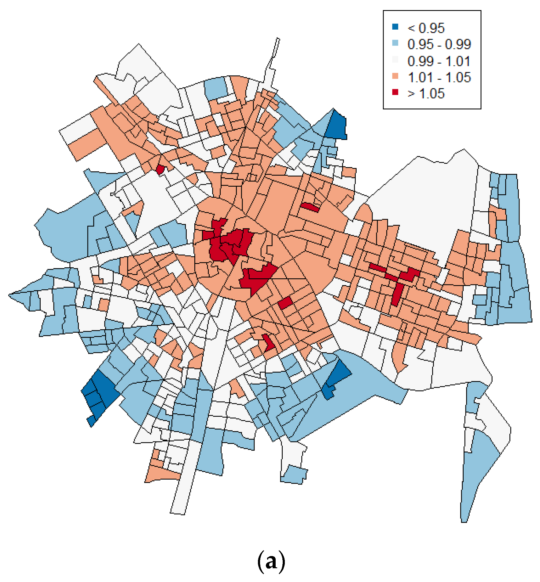
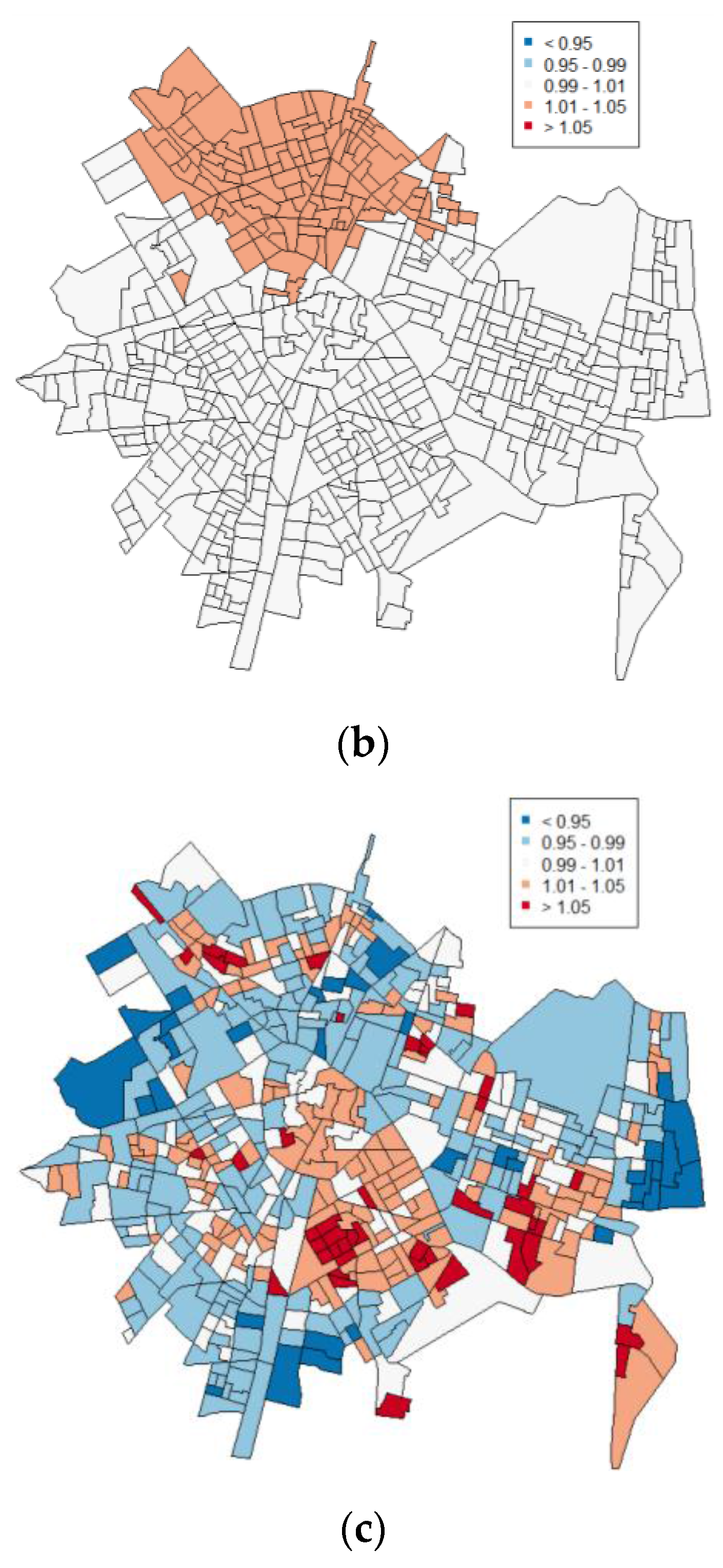
Our study also showed the spatiotemporal trends of alcohol outlets from 2010 to 2015. Off-premises and bars models showed a clear improvement in fit when introducing a spatiotemporal structure, and only restaurants/cafes showed a better fit using only a spatial model, suggesting different space-time patterns depending on the alcohol outlet category. For example, during this time period, off-premise density increased in the central and eastern part of the city, and decreased in the peripheral areas. On the other hand, bar density increased in the south-central part of the city. This area corresponds to one of the traditional neighborhoods of Valencia, which has become a trendy district for the city’s nightlife after a process of gentrification [56], which may explain the significant increase in bars in the area. Restaurant/cafe density, however, did not show important changes over the years, suggesting stable density levels.

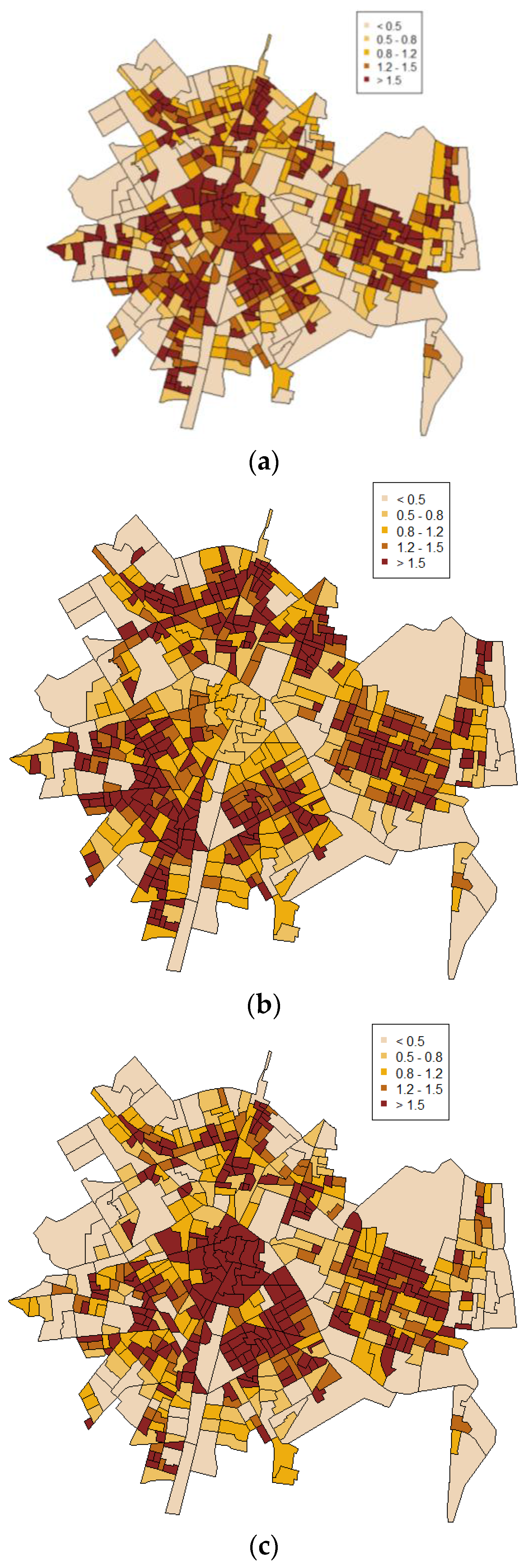
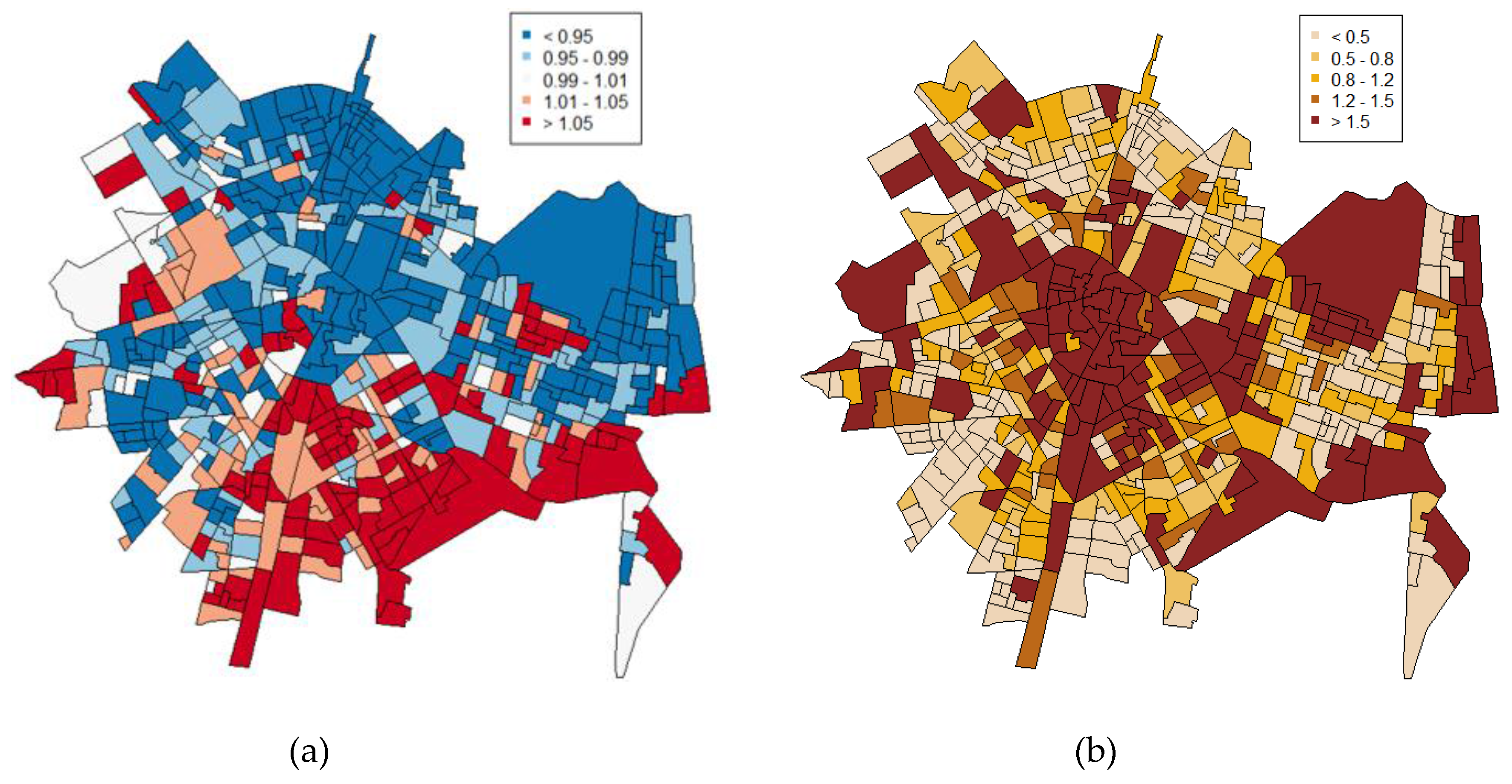
To examine whether alcohol outlets were associated with alcohol-related problems in the neighborhoods, we also analyzed the influence of alcohol outlet density on alcohol-related calls-for-service. Results showed that bar density was the only alcohol outlet category with a positive association with alcohol-related calls-for-service risks. Restaurant/cafe density showed a negative relationship. Off-premise establishments showed no association with alcohol-related calls-for-service. When comparing the spatial distribution of alcohol-related calls-for-service and alcohol outlets, we can observe that the spatial pattern of alcohol-related calls-for-service is similar to the spatial distribution of bars. Specifically, the centre of the city showed higher relative risk of alcohol-related calls-for-service, as well as higher bar density. In addition, the temporal trend for calls-for-service (increasing in the south areas and decreasing in the north areas) is more coincident with the temporal trend for bars, which shows the same change patterns.

These findings show that police alcohol-related interventions are more common in neighborhoods with a higher density of bars. Despite the fact that these high bar-density areas are located in higher-income areas, police interventions are requested more often in these areas due to alcohol-related problems. This is similar to the context in the U.S., where bars are related to a variety of crimes [6,19]; although those studies did not measure only alcohol-related crimes. However, off-premise density was not related to alcohol-related calls-for-service. In the U.S., off-premise establishments are seen as an indicator of a “spiral of decay” that leads to more social problems, such as violent crime or injuries [8,57,58,59]. These differences between Spain and U.S. cities could be explained by the different meaning of off-premise establishments in Spain. In a wet country like Spain, the sale of alcohol does not require strict conditions, and alcohol is easily available in many establishments, including supermarkets, grocery stores, petrol stations, or small stores, where they are usually displayed along with nonalcoholic beverages. Spain, and by extension, wet drinking countries, would have the off-premise sale of alcohol more integrated into social life. These differences regarding off-premises may also be due to the fact that our study only assessed alcohol-related crimes. The U.S. studies tend to focus on all crimes within a specified area. As off-premise outlets do not allow alcohol use on premise, the number of alcohol-related crimes may actually be unaffected. In addition, wealthy neighborhoods may be more likely to call the police, because they may show greater trust in the police system, or because the police could be more likely to respond promptly in this type of neighborhoods than in deprived neighborhoods. However, we do not have available data to assess these possible relationships. Cross-cultural studies are needed to further analyze these differences and the implications of alcohol outlets in social problems.

This study has both strengths and limitations. Among the strengths, to the best of our knowledge, this is the first study on the spatial-temporal distribution of alcohol outlets in a city from a “wet” country. Most of the research in this field has been conducted in U.S. or northern European countries. Our results show that the influence of neighborhood-level variables on the distribution of alcohol outlets could be different in southern European cities, and that it is important to take into account the country’s drinking culture to make appropriate conclusions. In addition, this study uses a spatiotemporal perspective. This type of analysis presents major advantages because it reflects not only the spatial distribution, but it also accounts for changes over time. Studies that only consider spatial trends could bias the results and mask any relationship between variables [49]. In addition, we use a Bayesian perspective, and we introduced different random-effects accounting for both spatial and temporal influences. Bayesian modelling has the advantage of addressing issues such as spatial autocorrelation or overdispersion, which can bias estimates if not taken into account [60,61,62]. Finally, this study provides information about alcohol outlet distribution in small areas. Some studies have focused on larger areas such as zip codes, census tracks, or counties [7,26,63]; we used census block groups, which were the smallest spatial unit available. This high-spatial resolution approach addressed potential issues in ecological studies due to aggregation effects [62].

This study has also limitations. First, some traditional variables used for characterizing neighborhoods were not available for this study; for example, other socioeconomic indicators used in previous research that may reflect the better economic status of the census block groups (e.g., income, unemployment, or poverty indicators [19,25,28,29]), or variables related to neighborhood disorder [64,65]. In addition, we cannot discard that some endogeneity may exist in the relationship between bars, crime, and property values. For example, property values may be a product of overall crime rates in the area. Future research should address the possible nonrecursive relationship between these variables, and study the causality processes that would be explaining the results found in this study.

Regarding methodological aspects, a potential issue is the modifiable areal unit problem [66]. In addition, our analysis may also be subjected to edge effect, where spillovers into surrounding rural areas around Valencia are not included in our model [5,67]. Another possible limitation is that, due to the short number of years available, we have used a linear time trend. However, other alternative and more complex models may be more appropriate and reveal more information about the problem when using longer time periods, such as an autoregressive structure or other nonlinear space-time models [51,52,68].

In addition, it is important to note that alcohol-related calls refer only to those cases where police are required to intervene for alcohol-related problems, and they do not reflect other outcomes, such as hospital admissions, where the police do not intervene, or traffic crashes where alcohol is involved, which were not available for this study. Future research would benefit from focusing on other alcohol-related outcomes and explore their relationships with alcohol outlet density. In addition, more research is needed in the context of wet drinking countries, in order to analyze if they show the same sociospatial patterns, which differ from those found in dry drinking countries.

5. Conclusions

This is the first study focused on the spatiotemporal distribution of alcohol outlets in a city from a wet drinking country, and its relationship with alcohol-related calls-for-service. After analyzing the different categories of alcohol outlets, we can conclude that they present different space-time distributions, as well as different associations with neighborhood-level characteristics. This suggests that an aggregated measure of total alcohol outlet density would not be appropriate, and future studies that use alcohol outlets to study social outcomes in a wet country should take into account each category separately.

Our results regarding alcohol-related calls-for-service could be of help for planning and evaluating prevention policies for alcohol-related police interventions, focusing on those places with high density of bars, which show more alcohol-related problems that require police intervention.

Future studies should focus on using these alcohol outlets categories to explain different social problems (i.e., intimate partner violence or child maltreatment) after controlling for social disorganization traditional variables (e.g., socioeconomic status, immigrant concentration, or residential instability). In addition, future studies should focus on analyzing whether the influence of alcohol outlet density in neighborhood social problems in wet countries follow the same patterns as those found in previous studies conducted in dry drinking countries.

References

1. Britt, H.R.; Carlin, B.P.; Toomey, T.L.; Wagenaar, A.C. Neighborhood level spatial analysis of the relationship between alcohol outlet density and criminal violence. Environ. Ecol. Stat. 2005, 12, 411–426. [Google Scholar] [CrossRef]
2. World Health Organization. Global Status Report on Alcohol and Health; World Health Organization: Luxemburg, 2014. [Google Scholar]
3. Campbell, C.A.; Hahn, R.A.; Elder, R.; Brewer, R.; Chattopadhyay, S.; Fielding, J. The effectiveness of limiting alcohol outlet density as a means of reducing excessive alcohol consumption and alcohol-related harms. Am. J. Prev. Med. 2009, 37, 556–569. [Google Scholar] [CrossRef] [PubMed]
4. White, G.F.; Gainey, R.R.; Triplett, R.A. Alcohol outlets and neighborhood crime: A longitudinal analysis. Crime Delinquency 2015, 61, 851–872. [Google Scholar] [CrossRef]
5. Cameron, M.P.; Cochrane, W.; Gordon, C.; Livingston, M. Alcohol outlet density and violence: A geographically weighted regression approach. Drug Alcohol Rev. 2016, 35, 280–288. [Google Scholar] [CrossRef] [PubMed]
6. Gorman, D.M.; Speer, P.W.; Gruenewald, P.J.; Labouvie, E.W. Spatial dynamics of alcohol availability, neighborhood structure and violent crime. J. Stud. Alcohol 2001, 62, 628–636. [Google Scholar] [CrossRef] [PubMed]
7. Gruenewald, P.J.; Remer, L. Changes in outlet densities affect violence rates. Alcohol. Clin. Exp. Res. 2006, 30, 1184–1193. [Google Scholar] [CrossRef] [PubMed]
8. Furr-Holden, C.D.M.; Milam, A.J.; Nesoff, E.D.; Johnson, R.M.; Fakunle, D.O.; Jennings, J.M.; Thorpe, R.J. Not in my back yard: A comparative analysis of crime around publicly funded drug treatment centers, liquor stores, convenience stores, and corner stores in one Mid-Atlantic City. J. Stud. Alcohol Drugs 2016, 77, 17–24. [Google Scholar] [CrossRef] [PubMed]
9. Popova, S.; Giesbrecht, N.; Bekmuradov, D.; Patra, J. Hours and days of sale and density of alcohol outlets: Impacts on alcohol consumption and damage: A systematic review. Alcohol Alcohol. 2009, 44, 500–516. [Google Scholar] [CrossRef] [PubMed]
10. Treno, A.J.; Johnson, F.W.; Remer, L.G.; Gruenewald, P.J. The impact of outlet densities on alcohol-related crashes: A spatial panel approach. Accid. Anal. Prev. 2007, 39, 894–901. [Google Scholar] [CrossRef] [PubMed]
11. LaScala, E.A.; Johnson, F.W.; Gruenewald, P.J. Neighborhood characteristics of alcohol-related pedestrians injury collisions: A geostatistical analysis. Prev. Sci. 2001, 2, 123–134. [Google Scholar] [CrossRef] [PubMed]
12. McKinney, C.M.; Chartier, K.G.; Caetano, R.; Harris, T.R. Alcohol availability and neighborhood poverty and their relationship to binge drinking and related problems among drinkers in committed relationships. J. Interpers. Violence 2012, 27, 2703–2727. [Google Scholar] [CrossRef] [PubMed]
13. Foster, S.; Trapp, G.; Hooper, P.; Oddy, W.H.; Wood, L.; Knuiman, M. Liquor landscapes: Does access to alcohol outlets influence alcohol consumption in young adults? Health Place 2017, 45, 17–23. [Google Scholar] [CrossRef] [PubMed]
14. Azar, D.; White, V.; Coomber, K.; Faulkner, A.; Livingston, M.; Chikritzhs, T.; Room, R.; Wakefield, M. The association between alcohol outlet density and alcohol use among urban and regional Australian adolescents. Addiction 2015, 111, 65–72. [Google Scholar] [CrossRef] [PubMed]
15. Rowland, B.; Evans-Whipp, T.; Hemphill, S.; Leung, R.; Livingston, M.; Toumbourou, J.W. The density of alcohol outlets and adolescent alcohol consumption: An Australian longitudinal analysis. Health Place 2016, 37, 43–49. [Google Scholar] [CrossRef] [PubMed]
16. Freisthler, B.; Weiss, R.E. Using Bayesian space-time models to understand the substance use environment and risk for being referred to child protective services. Subst. Use Misuse 2008, 43, 239–251. [Google Scholar] [CrossRef] [PubMed]
17. Freisthler, B.; Gruenewald, P.J.; Treno, A.J.; Lee, J. Evaluating alcohol access and the alcohol environment in neighborhood areas. Alcohol. Clin. Exp. Res. 2003, 27, 477–484. [Google Scholar] [CrossRef] [PubMed]
18. Freisthler, B.; Kepple, N.J.; Holmes, M.R. The geography of drug market activities and child maltreatment. Child Maltreatment 2012, 17, 144–152. [Google Scholar] [CrossRef] [PubMed]
19. Cunradi, C.B.; Mair, C.; Ponicki, W.; Remer, L. Alcohol outlets, neighborhood characteristics, and intimate partner violence: Ecological analysis of a California city. J. Urban Health 2011, 88, 191–200. [Google Scholar] [CrossRef] [PubMed]
20. Snowden, A.J. Alcohol outlet density and intimate partner violence in a nonmetropolitan college town: Accounting for neighborhood characteristics and alcohol outlet types. Violence Vict. 2016, 31, 111–123. [Google Scholar] [CrossRef] [PubMed]
21. Angus, C.; Holmes, J.; Maheswaran, R.; Green, M.A.; Meier, P.; Brennan, A. Mapping patterns and trends in the spatial availability of alcohol using low-level geographic data: A case study in England 2003–2013. Int. J. Environ. Res. Public Health 2017, 14, 406. [Google Scholar] [CrossRef] [PubMed]
22. Ellaway, A.; Macdonald, L.; Forsyth, A.; Macintyre, S. The socio-spatial distribution of alcohol outlets in Glasgow city. Health Place 2010, 16, 167–172. [Google Scholar] [CrossRef] [PubMed]
23. Han, D.; Gorman, D.M. Socio-spatial patterning of off-sale and on-sale alcohol outlets in a Texas City. Drug Alcohol Rev. 2014, 33, 152–160. [Google Scholar] [CrossRef] [PubMed]
24. Shaw, C.R.; McKay, H.D. Juvenile Delinquency and Urban Areas; University of Chicago Press: Chicago, IL, USA, 1942. [Google Scholar]
25. Sampson, R.J.; Raudenbush, S.W.; Earls, F. Neighborhoods and violent crime: A multilevel study of collective efficacy. Science 1997, 277, 918–924. [Google Scholar] [CrossRef] [PubMed]
26. Bursik, R.J. Social disorganization and theories of crime and delinquency: Problems and prospects. Criminology 1988, 26, 519–552. [Google Scholar] [CrossRef]
27. Hay, G.C.; Whigham, P.A.; Kypri, K.; Langley, J.D. Neighborhood deprivation and access to alcohol outlets: A national study. Health Place 2009, 15, 1086–1093. [Google Scholar] [CrossRef] [PubMed]
28. Shimotsu, S.T.; Jones-Webb, R.J.; MacLehose, R.F.; Nelson, T.F.; Forster, J.L.; Lytle, L.A. Neighborhood socioeconomic characteristics, the retail environment, and alcohol consumption: A multilevel analysis. Drug Alcohol Depend. 2013, 132, 449–456. [Google Scholar] [CrossRef] [PubMed]
29. Bluethenthal, R.N.; Deborah, C.A.; Farley, T.A.; Scribner, R.; Beighley, C.; Schonlau, M.; Robinson, P.L. Alcohol availability and neighborhood characteristics in Los Angeles, California and Southern Louisiana. J. Urban Health 2008, 85, 191–205. [Google Scholar] [CrossRef] [PubMed]
30. Nielsen, A.L.; Hill, T.D.; French, M.T.; Hernandez, M.N. Racial/ethnic composition, social disorganization, and offsite alcohol availability in San Diego County, California. Soc. Sci. Res. 2010, 39, 165–175. [Google Scholar] [CrossRef] [PubMed]
31. Snowden, A.J. Neighborhood characteristics contribute to urban alcohol availability: Accounting for race/ethnicity and social disorganization. J. Ethn. Subst. Abuse 2016, 15, 346–366. [Google Scholar] [CrossRef] [PubMed]
32. LaVeist, T.A.; Wallace, J.M. Health risk and inequitable distribution of liquor stores in African American neighborhood. Soc. Sci. Med. 2000, 51, 613–617. [Google Scholar] [CrossRef]
33. Gorman, D.M.; Speer, P.W. The concentration of liquor outlets in an economically disadvantaged city in the Northeastern United States. Subst. Use Misuse 1997, 32, 2033–2046. [Google Scholar] [CrossRef] [PubMed]
34. Zhang, X.; Hatcher, B.; Clarkson, L.; Holt, J.; Bagchi, S.; Kanny, D.; Brewer, R.D. Changes in density of on-premises alcohol outlets and impact on violent crime, Atlanta, Georgia, 1997–2007. Prev. Chronic Dis. 2015, 12, E84. [Google Scholar] [CrossRef] [PubMed]
35. Rahav, G.; Wilskack, R.; Bloomfield, K.; Gmel, G.; Kuntsche, S. The influence of societal level factors on men’s and women’s alcohol consumption and alcohol problems. Alcohol Alcohol. 2006, 41, i47–i55. [Google Scholar] [CrossRef] [PubMed]
36. Room, R.; Mitchell, A. Notes on cross-national and cross-cultural studies. Drink. Drug Pract. Surv. 1972, 5, 16–20. [Google Scholar]
37. Room, R.; Mäkela, K. Typologies of the cultural position of drinking. J. Stud. Alcohol 2000, 61, 475–483. [Google Scholar] [CrossRef] [PubMed]
38. Mäkela, P.; Gmel, G.; Grittner, U.; Kuendig, H.; Kuntsche, S.; Bloomfield, K.; Room, R. Drinking patterns and their gender differences in Europe. Alcohol Alcohol. 2006, 41, i8–i18. [Google Scholar] [CrossRef] [PubMed]
39. Allamani, A.; Voller, F.; Kubicka, L.; Bloomfield, K. Drinking cultures and the position of women in nine European countries. Subst. Abuse 2000, 21, 231–247. [Google Scholar] [CrossRef] [PubMed]
40. Jose, A.; O’Leary, D.; Graña Gomez, J.L.; Foran, H.M. Risk factors for men’s intimate physical aggression in Spain. J. Fam. Violence 2014, 29, 289–297. [Google Scholar] [CrossRef]
41. Bloomfield, K.; Stockwell, T.; Gmel, G.; Rehn, N. International comparisons of alcohol consumption. Alcohol Res. Health 2003, 27, 95–109. [Google Scholar] [PubMed]
42. BOP Consulting. The World Cities Culture Report 2014; Public Liaison Unit: London, UK, 2015. [Google Scholar]
43. Gruenewald, P.J.; Freisthler, B.; Remer, L.; LaScala, E.A.; Treno, A. Ecological models of alcohol outlets and violent assaults: Crime potentials and geospatial analysis. Addiction 2006, 101, 666–677. [Google Scholar] [CrossRef] [PubMed]
44. Freisthler, B.; Midanik, L.T.; Gruenewald, P.J. Alcohol outlets and child physical abuse and neglect: Applying routine activities theory to the study of child maltreatment. J. Stud. Alcohol Drugs 2004, 65, 586–592. [Google Scholar] [CrossRef]
45. Freisthler, B. A spatial analysis of social disorganization, alcohol access, and rates of child maltreatment in neighborhoods. Child. Youth Serv. Rev. 2004, 26, 803–819. [Google Scholar] [CrossRef]
46. Rosso, A.L.; Grubesic, T.H.; Auchincloss, A.H.; Philip-Tabb, L.; Michael, Y.L. Neighborhood amenities and mobility in older adults. Am. J. Epidemiol. 2013, 178, 617–637. [Google Scholar] [CrossRef] [PubMed]
47. Anselin, L. Under the hood issues in the specification and interpretation of spatial regression models. Agric. Econ. 2002, 27, 247–267. [Google Scholar] [CrossRef]
48. Morrison, C.M.; Gruenewald, P.J.; Ponicki, W.R. Socioeconomic determinants of exposure to alcohol outlets. J. Stud. Alcohol. Drugs 2015, 76, 439–446. [Google Scholar] [CrossRef] [PubMed]
49. Lawson, A.B.; Brown, W.J.; Vidal Rodeiero, C.L. Disease Mapping with WinBUGS and MLwiN; John Wiley & Sons Ltd.: New York, NY, USA, 2003. [Google Scholar]
50. Li, G.; Haining, R.; Richardson, S.; Best, N. Space-time variability in burglary risk: A Bayesian spatio-temporal modelling approach. Spat. Stat. 2014, 9, 180–191. [Google Scholar] [CrossRef]
51. Martínez-Beneito, M.A.; López-Quílez, A.; Botella-Rocamora, P. An autoregressive approach to spatio-temporal disease mapping. Stat. Med. 2008, 27, 2874–2889. [Google Scholar] [CrossRef] [PubMed]
52. Spiegelhalter, D.J.; Best, N.G.; Carlin, B.P.; van der Linde, A. Bayesian measures of model complexity and fit. J. R. Stat. Soc. B 2002, 64, 583–639. [Google Scholar] [CrossRef]
53. Marco, M.; López-Quílez, A.; Conesa, D.; Gracia, E.; Lila, M. Spatio-temporal analysis of suicide-related emergency calls. Int. J. Environ. Res. Public Health 2017, 14, 735. [Google Scholar] [CrossRef] [PubMed]
54. Luan, H.; Quick, M.; Law, J. Analyzing local spatio-temporal patterns of police calls-for-service using Bayesian Integrated Nested Laplace Approximation. ISPRS Int. J. Geo-Inf. 2016, 5, 162. [Google Scholar] [CrossRef]
55. Besag, J.; York, J.; Mollié, A. Bayesian image restoration, with two applications in spatial statistics. Ann. I. Stat. Math. 1991, 43, 1–20. [Google Scholar] [CrossRef]
56. Del Romero, L.; Lara, L. Ward—Problem sweeping fashion: Commercial gentrification Russa-fa, the valencian ‘Soho’. An. Geogr. 2015, 35, 187–212. [Google Scholar]
57. Zhu, L.; Gorman, D.M.; Horel, S. Alcohol outlet density and violence: A geospatial analysis. Alcohol Alcohol. 2004, 39, 369–375. [Google Scholar] [CrossRef] [PubMed]
58. Fone, D.; Morgan, J.; Fry, R.; Rodgers, S.; Orford, S.; Farewell, D.; Dunstan, F.; White, J.; Sivarajasingam, V.; Trefan, L.; et al. Change in alcohol outlet density and alcohol-related harm to population health (CHALICE). BMC Public Health 2012, 12, 428. [Google Scholar] [CrossRef] [PubMed]
59. Morrison, C.; Smith, K.; Gruenewald, P.J.; Ponicki, W.R.; Lee, J.P.; Cameron, P. Relating off-premises alcohol outlet density to intentional and unintentional injuries. Addiction 2016, 111, 56–64. [Google Scholar] [CrossRef] [PubMed]
60. Gracia, E.; López-Quílez, A.; Marco, M.; Lladosa, S.; Lila, M. The spatial epidemiology of intimate partner violence: Do neighborhoods matter? Am. J. Epidemiol. 2015, 182, 58–66. [Google Scholar] [CrossRef] [PubMed]
61. Bernardinelli, L.; Clayton, D.; Pascutto, C.; Montomoli, C.; Ghislandi, M.; Songini, M. Bayesian analysis of space-time variation in disease risk. Stat. Med. 1995, 14, 2433–2443. [Google Scholar] [CrossRef] [PubMed]
62. Lawson, A.B. Bayesian Disease Mapping: Hierarchical Modeling in Spatial Epidemiology; CRC Press: Boca Raton, FL, USA, 2009. [Google Scholar]
63. Lipton, R.; Gruenewald, P. The spatial dynamics of violence and alcohol outlets. J. Stud. Alcohol 2002, 63, 187–195. [Google Scholar] [CrossRef] [PubMed]
64. Marco, M.; Gracia, E.; Tomás, J.M.; López-Quílez, A. Assessing neighborhood disorder: Validation of a three-factor observational scale. Eur. J. Psychol. Appl. Leg. Context 2015, 7, 81–90. [Google Scholar] [CrossRef]
65. Marco, M.; Gracia, E.; Martín-Fernández, M.; López-Quílez, A. Validation of a Google Street View-based neighborhood disorder observational scale. J. Urban Health 2017, 94, 190–198. [Google Scholar] [CrossRef] [PubMed]
66. Heywood, I.; Cornelius, S.; Carver, S. Introduction to Geographical Information Systems; Adission Wesley Longman: New York, NY, USA, 1998. [Google Scholar]
67. Cameron, M.P.; Cochrane, W.; Gordon, C.; Livingston, M. Global and locally-specific relationships between alcohol outlet density and property damage: Evidence from New Zealand. Austral. J. Reg. Stud. 2016, 22, 331–354. [Google Scholar]
68. Gracia, E.; López-Quílez, A.; Marco, M.; Lila, M. Mapping child maltreatment risk: A 12-year spatio-temporal analysis of neighborhood influences. Int. J. Health Geogr. 2017, 16, 38. [Google Scholar] [CrossRef] [PubMed]
Figure 1. (a) Change in off-premise density from 2010 to 2015; (b) change in restaurant/cafe density from 2010 to 2015; and (c) change in bar density from 2010 to 2015.
Ijgi 06 00380 g001aIjgi 06 00380 g001b
Figure 2. (a) Off-premise density in 2015; (b) restaurant/cafe density in 2015; and (c) bar density in 2015.
Ijgi 06 00380 g002
Figure 3. (a) Change in alcohol-related calls-for-service from 2010 to 2015; and (b) the relative risk of alcohol-related calls-for-service in 2015.
Ijgi 06 00380 g003