Machine Learning Techniques for Modelling Short Term Land-Use Change


1
Faculty of Civil Engineering, University of Belgrade, Bulevar kralja Aleksandra 73, 11000 Belgrade, Serbia
2
Spatial Analysis and Modeling Laboratory, Department of Geography, Simon Fraser University, 8888 University Drive, Burnaby, BC V5A 1S6, Canada
*
Authors to whom correspondence should be addressed.
ISPRS Int. J. Geo-Inf. 2017, 6(12), 387; https://doi.org/10.3390/ijgi6120387
Submission received: 31 October 2017
/
Revised: 24 November 2017
/
Accepted: 26 November 2017
/
Published: 29 November 2017
Abstract
:The representation of land use change (LUC) is often achieved by using data-driven methods that include machine learning (ML) techniques. The main objectives of this research study are to implement three ML techniques, Decision Trees (DT), Neural Networks (NN), and Support Vector Machines (SVM) for LUC modeling, in order to compare these three ML techniques and to find the appropriate data representation. The ML techniques are applied on the case study of LUC in three municipalities of the City of Belgrade, the Republic of Serbia, using historical geospatial data sets and considering nine land use classes. The ML models were built and assessed using two different time intervals. The information gain ranking technique and the recursive attribute elimination procedure were implemented to find the most informative attributes that were related to LUC in the study area. The results indicate that all three ML techniques can be used effectively for short-term forecasting of LUC, but the SVM achieved the highest agreement of predicted changes.
1. Introduction
Studying, understanding, and modeling the land use change (LUC) process is important and represents one of the key research topic for many disciplines, particularly geography, urban planning, geo-information science, ecology, and land use science [1,2,3]. Understanding the spatial patterns of the LUC process can enable planners and policy-makers to manage community development and growth in a sustainable way. LUC is influenced by many driving factors, ranging from socio-economic conditions, demography, landscape topography, physical infrastructure, and planning constraints and policies. Consequently, modeling the LUC process is a challenging undertaking that has been implemented using various techniques, from logistic and multiple regression [4,5,6], Markov models [7,8], cellular automata [9,10,11], agent-based approaches [12,13], and more recently, machine learning (ML) techniques [14,15]. Modeling the LUC process is dependent on availability of various and large data sets including demographic, geospatial, and historical data, and can be expressed as being data-driven.
The main focus of data-driven modeling methods is to find patterns and trends or to induce representative models of underlying processes using past data [16,17]. These modeling methods assume stationarity in the relationship between the predictors and land change variables [18]. Consequently, it is possible to discover the relationship between process inputs and outputs without the need for detailed understanding of the physical transformation process or transition functions. The discovered relationships between the inputs and outputs are then used to define a model with only a limited number of assumptions [19]. These properties make data-driven models easily transferrable to various end-user contexts when compared with related agent-based or cellular automata models that normally require expert knowledge to define the transition rules.
In the last decade, increases in data acquisition technologies and higher computation capacities have resulted in numerous research studies exploring data-driven approaches. ML is a data-driven approach that is successfully implemented in different geoscience disciplines, such as: hydrology [19,20]; geology [21,22,23]; ecology [24,25,26]; and, remote sensing [27,28,29]. Moreover, comparative studies have been in rise that particularly examine two or more of the available ML techniques within specific application and data availability contexts [30,31,32,33,34,35,36].
LUC is a complex process, and hence, ML provides suitable tools to represent the change process. The early ML techniques applied to LUC modeling used artificial neural networks, coupled with cellular automata [37,38] and geographic information system (GIS) [39,40]. In addition, Decision Trees [41] and Support Vector Machines were used to guide transition rules for cellular automata models [42,43]. Modeling LUC using ML techniques, such as Decision Trees, Support Vector Machines, Neural Network, and Random Forest have been expanding in recent years [15,44,45,46]. The LUC models described in these studies used only one ML technique and considered only two or three land use classes. Tayyebi and Pijanowski [14] used three ML techniques: Neural Network, Classification and Regression Trees, and Multivariate Adaptive Regression Splines for modeling land use changes when considering four land use class: (1) agriculture, (2) urban, (3) forest, and (4) other classes. They concluded that Neural Networks (NN) provided a better accuracy when comparing with the other two techniques. However, they used the same time interval in order to train and test the model. Further, many of those mentioned studies focused on the correlations between spatial indicators and land use classes at the same time point, but they do not extend toward estimating LUC to forecast or how it is often titled in statistical terms to predict the near future. ML frameworks that used to build such models are readily transferable to different urban environments, and, except for data preparation that could be automated, would require the limited involvement of a knowledge expert. Therefore, this research study addresses two main objectives regarding forecasting short-term land use class changes using ML techniques; selecting appropriate data representation and comparison of selected outputs of nine urban land use class models derived by three ML techniques, Decision Trees (DT), Neural Networks (NN) and Support Vector Machines (SVM).
Given that the proposed models use past data to “learn” the unknown relations between predictor variables and nine land use classes, it is a necessary requirement to define how the entities from the real world are described by choosing the most informative attributes (predictors) for the problem at hand. In our case study, the focus in on spatial attributes only, but other information categories, such as socio-economic position, could be easily added to the model building framework. The attribute selection process provides benefits, such as improving model accuracy, reducing noisy inputs and model complexity, and finally reducing the time required for training [47,48,49,50]. Informative attributes were selected using the Information Gain ranking technique and the procedure of recursive attribute elimination.
The performance of three commonly used ML classification algorithms (DT, NN, and SVM) were assessed using the Sensitivity (True Positive rate—TPrate), Fall-out (False Positive rate—FPrate), Area Under Receiver Operating Characteristic Curve (AUC) [51] measure, and the method of comparison of three maps [52]. The rationale for selecting a particular classification algorithm was based on high classification accuracy in many domains (NN, SVM) and easy model interpretability (DT). The forecasting land use models were tested on multiple land use class transitions that characterized different urban growth behaviours within the City of Belgrade, Republic of Serbia. A total of nine land use classes were investigated using data from three selected municipalities in the City of Belgrade for the time interval 2001–2011. The models were built and tested using two different time intervals 2003–2007 and 2007–2011, respectively.
In the sections that follow, we formally define the classification problem for LUC forecasting, outline the work-flow developed for designing the models (attribute selection and learning protocol), report on the model comparison results, and provide conclusions from the research work.
2. Methods
2.1. Formulating the Problem as a Classification Task
In order to build a predictive short-term LUC model using ML techniques, it is necessary to have series of historical data for the study area in consideration and the assumption that an unknown land use transition function retains similar properties over a short time interval for which the model is generated. Generally, the duration of the short time interval depends on the properties of the study area. For our chosen study area, it takes three to four years. LUC models that are based on ML require the transformation of physical, socio-economic, neighboring, and other related data for each spatial cell unit of the study area into an appropriate data representation. The study area is usually represented as a grid of cells that are georeferenced as raster data layers in a geographic information system (GIS). Each raster cell has a regular shape, usually square, with its accompanying attributes and land use class. Several GIS data layers of the study area at different time points are necessary to build ML models for LUC analysis. The ML technique for modeling LUC can be regarded as a classification problem [53], which is more formally defined as follows:
Let C = {c1, c2, …, ck} be the set of k predefined land use classes. Each grid cell at time point t can be represented as a row vector xt = <xt1,…, xti,…, xtn> with xti representing the value of the i-th spatial attribute that is assigned to the cell. Further, let yt from C be a land use class of xt at time point t. A function fp: xt → yt+1 applied over each xt from a grid representing the study area, is called a prediction if for each xt the relationship fp (xt) = yt+1 is true whenever a cell xt changes its land use to the class yt+1. Values from C are mapped into natural numbers, each representing a particular land use class. The model constraint is that each cell can belong to only one class at any time point t.
Assuming that the transition function fp exists and maps the grid at the time point t to land use classes at time point t + 1, the ML technique attempts to learn the function fp’ that approximates the unknown fp using only the training set in which all of the attribute values at time t and land use classes at time t + 1 are known beforehand. In order to evaluate the predictive power of the approximation, it is necessary to test the model that is built in the previous step with inputs xt+1 and to compare fp’(xt+1) with known yt+2. Hence, model building and validation assumes the availability of data on spatial attributes and land use classes from three different time points [18].
2.2. Forecasting Short-Term Land Use Change Based on ML Techniques
The applied methodology for model building and verification consisted of five steps: (1) creating the initial geospatial data set; (2) creating training and test data sets; (3) attribute ranking; (4) model building for each ML technique; and, (5) model validation.
Step 1: Creating an initial input data set assumes the definition of a data representation for each grid cell xt at each time point t as discussed, in Section 2.1. The initial data set It, t+1 is created for each time interval (t, t + 1) containing xt represented with attributes and yt+1 as a land use class at time point t+1 for each cell in the study area.
Step 2: In order to learn the predictive function fp′, a training set of the form {(xt, yt+1)i}, i = 1,2,…,n, (n is the number of samples in the training set), was constructed from the initial set (It, t+1), where xit represents a grid cell at time point t and yit+1 represents its land use class at time point t + 1. Models that were obtained in the training phase were tested using an independent test set in the form of {(xt+1, yt+2)i}, i = 1,2,…,m (m is the number of samples in the test set). The test set was derived from the corresponding It+1, t+2 initial set. Note the necessity of using data from three different time points when building (t, t + 1) and testing (t + 1, t + 2) the proposed forecasting models.
Due to the large volume of data and the low percentage of cells that change their land use class over time, the most commonly used random sampling is not appropriate. Therefore, we applied a balanced sampling strategy [54], providing more informative data sets for the supervised learning algorithm and building models that are less affected by unchanged cells or majority classes. The balanced training and test sets were created from the initial data sets in the following manner: (a) all of the cells that change their class were selected together with the same number of cells without LUC, (b) unchanged cells were chosen to be uniformly distributed across the whole area, and (c) the proportion of all the land-use classes remained the same as in the initial sets. Balanced training and test sets were labeled as St, t+1 (training) and St+1, t+2 (test).
Step 3: The goal of attribute ranking is to choose a subset of input attributes by eliminating those with small or no predictive influence on the model output. These less important attributes lower the performance of the ML process [48]. The Info Gain (IG) ranking method that was used in this research is based on the concept of entropy that is defined in information theory [55]. It provides the concept of how much information gained towards a correct classification is obtained if the value of the selected attribute is known. The IG ranking method independently evaluates all of the attributes using the training set and provides their ranking for the classification problem at hand. We applied a recursive attribute elimination method [56] and IG ranking to analyse the impact of the n most informative attributes on model performance.
Step 4: After selecting the appropriate spatial attributes and creating a balanced training and test sets from the initial data, the next step was to build classification models using DT, NN, and SVM.
Step 5: In order to assess and compare various modeling outcomes that were obtained from the different ML techniques, the weighted averages of TPrate, FPrate and AUC measure [57], and for an in-depth analysis of comparison of the three maps method [52], were applied. The overall model performance can be represented by weighted averages of TPrate, FPrate, and AUC (Weighted AUC), in which weights could be selected appropriately (if weights are equal, all of the classes are equally important in model validation). The comparison of the three maps method is based on a three-dimensional table that is constructed by comparing land use classes in three maps: reference (real) map at time t+1, reference map at time t + 2, and simulation map at time t + 2. Pontius et al. [52] explained this concept in detail; generally, the three-dimensional table quantifies simultaneously the observed (real) and simulated transitions among different classes. The method examines two components of agreement and three components of disagreement. The agreement is measured through persistence simulated correctly and change simulated correctly, while the disagreement is observed as a change simulated as persistence, change simulated as change to wrong category, and persistence simulated as change. These quantities provide a clear insight into the forecasting capability of the model, by giving separate measures for the cells that changed their land use over the testing interval and for the ones that remained unchanged.
2.3. Machine Learning Techniques—Theoretical Background
The three ML techniques DT, NN, and SVM were used for supervised learning in order to build the LUC models and are briefly described as follows:
DT refers to hierarchical models that are used for classification and decision making [58]. A tree consists of decision nodes in which an instance is tested against the values of the associated attribute. The instance follows one of the possible paths from the root to a leaf node, where it is classified according to the majority of training examples that were associated with this leaf node. There are many different learning approaches that are used to build the tree from the training data, such as CART [59], ID3 [60], and C4.5 [61]. The C4.5 decision-tree classifier was adopted for use in this study since it uses a common strategy for tree induction from the training data [61], where the more informative attributes are located in the upper parts of the tree. The advantage of a DT model is in its transferability to a set of if-then rules that connect input attributes and class decisions, which are easily understandable for domain experts.
NN originate from the late 1950’s when Rosenblatt [62] presented the perceptron as the simplest form of the NN, which calculates the weighted sum of its inputs and generate 1 if the sum is greater the predefined threshold, otherwise 0. Since then, various types of neural networks were designed, such as Kohonen network [63], Radial Basis network [64], and Multi-layer Perceptron. In our multi-class problem setting (nine land use classes), the Multi-layer Perceptron (MLP) neural network, as defined by Rumelhart et al. [65] was adopted for use. The MLP is one of the most widely used neural networks [39], in which data paths from input to output units are strictly feed-forward [66]. The network model is represented with a set of real weights that are associated to the interconnections between perceptrons, and a learning procedure is applied, where, in each iteration, weights are updated according to a back-propagation algorithm in order to minimize the error between the outputs of the network and the desired values.
The SVM [67,68] is a linear binary classifier. Every n-class problem can be transformed into a sequence of n (one-versus-all) or n(n−1)/2 (one-versus-one) binary classification tasks by using different voting schemes that ultimately lead to a final decision [69]. SVM tries to construct the separation hyperplane between the training points of two classes such that the margin of separation is maximal. However, for non-linear cases, it first maps the points into a high dimensional space in which the linear separation is feasible. There exist many mapping or kernel functions from the original input space to the high dimensional feature space. In our study, the Radial Basis Function, also known as the Gaussian kernel [70], was used as it handles both linear and non-linear problem domains.
The Weka 3.6 software (Machine Learning Group at the University of Waikato, Hamilton, New Zealand) [71,72] was used to build all of the models based on DT, NN, and SVM techniques. Weka [72] is an open source software that implements various types of ML algorithms. In this research, J48 was used as a Java implementation of the C4.5 algorithm for learning DT, Sequential Minimal-Optimization algorithm for SVM learning, and a two-layer feed forward net with error back-propagation for NN. In addition, Weka contains data pre-processing modules, including tools for attributes selection, such as IG, used in this research.
3. Study Area and Data Sets
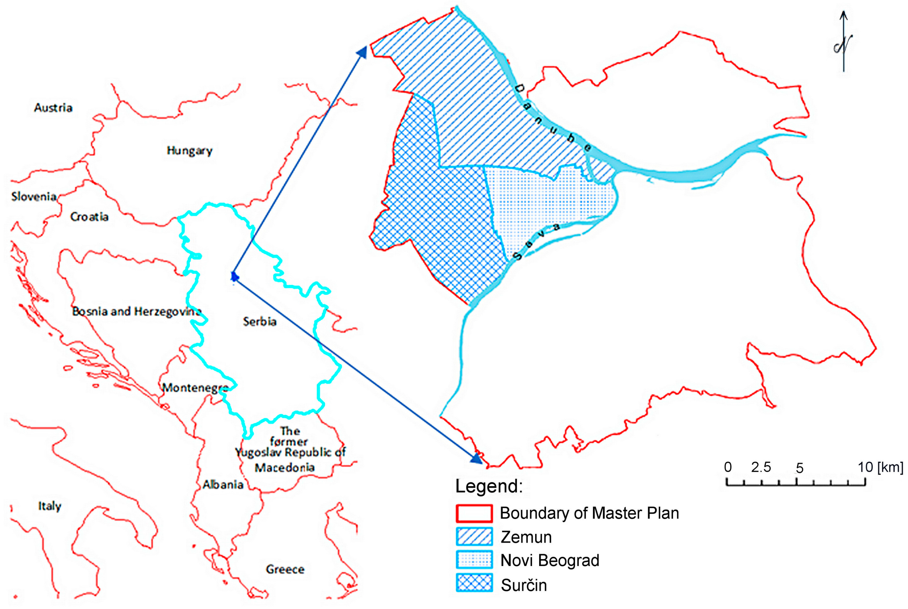
The City of Belgrade, in the Republic of Serbia, was developed under different cultural, historical, social, and economic influences that have shaped its urban morphology. The chosen study area includes three neighboring municipalities that are characterized by different urban dynamics: Zemun, Novi Beograd, and Surčin (Figure 1). The main study region covered an area of about 19 km × 25 km and was buffered by 100 m on each side to minimize any potential edge effects.
The spatial data were obtained from orthophoto images for the years 2001, 2003, 2007, and 2011, with spatial resolutions 0.30 × 0.30 m, 0.30 × 0.30 m, 0.25 × 0.25 m, 0.20 × 0.20 m, respectively, and from actual land use maps in vector format (*.shp files, polygons of land use class) that were provided from the Urban Planning Institute of Belgrade for the years 2001 and 2010. The maps of land use classes for the years 2003 and 2007 were created by digitizing corresponding orthophoto images. The maps of actual land use maps for the years 2001 and 2011, are created after correcting observed irregularities (such as overlapping polygons and undefined areas), and the detected changes occurred between years 2010 and 2011, based on a comparison of vector maps and corresponding orthophoto images.
The maps of land use for the years 2001 and 2010, represent 11 and 12 classes of land use, respectively. In order to define unique and consistent classification, the official 13 classes of land uses that were outlined in the 2021 Master Plan of Belgrade [73] were generalized into nine classes, when considering classification on actual land use maps from 2001 to 2010: Agricultural, Wetlands, Transportation networks, Infrastructure, Residential, Commercial, Industry, Special use, and Green areas. The data layer for each time point was georeferenced and integrated into a raster GIS database at a 10 m spatial resolution.
Supplementary maps representing spatial attributes were created to contain information on accessibility, population density, and spatial neighborhoods using available data that was mostly obtained from the Urban Planning Institute of Belgrade and via consultations with urban planners (Table 1). After the analysis of LUC trends for the considered time interval (2001–2011), the following accessibility maps were created to reflect distances from the: city center, municipality centers, rivers (Danube and Sava), green areas greater than 100 m × 100 m, railways, highways, main roads, and streets of category I and II. The accessibility maps refer to raster maps of Euclidean distance to the closest cell of interest, i.e., to the closest cell of rivers, green area, etc. The study area is relatively flat and so attributes that are related to elevation were not considered. Population counts were obtained for 2011 from the Serbian Census Office and the official estimated population for the years 2003 and 2007 were obtained from the Statistical Office of the Republic of Serbia. Population density was calculated for each grid cell using a dasymetric mapping method [74]. In order to emphasize the differences of urban types between three used municipalities (Zemun, New Belgrade and Surčin), an additional categorical attribute was defined containing information on cell location (the municipality of a cell), labeled as x1, Municipality code (Table 1).
The initial data set for each time interval, I2003,2007 and I2007,20011, contains attributes about the municipality code (Table 1, x1), Euclidian distances to specific entities (Table 1, x2–x10), population (Table 1, x11), the cell’s land use class (Table 1, x12), information about land use classes in the cell’s neighborhood (Table 1, x13 and x14), and information about the cell’s previous land use class (history) (Table 1, x15). The influence of neighboring cells (x13 and x14) is represented with the two most frequent classes within the nxn cells Moore neighborhood, which makes a link to cellular automata LUC models that utilise this type of information. The size of the neighborhood can be adjusted to fit various resolutions for different modeling areas. The conducted analysis suggested that 7 × 7 cells is the most suitable representation for local spatial neighborhoods, providing the best model performance results [54]. The information about the cell’s previous land use class clarified whether the past land use class influences future land use apart from the present class (cell’s memory info). As seen from the obtained research results, this type of information is important for the proposed models that are related to the study area. The previous land use class for the time interval 2003–2007 is land use class at the year 2001 and land use class at year 2003 represents previous land use class for the time interval 2007–2011.
Data preparation was performed using multiple software tools. The SAGA GIS environment [75] and ArcGIS [76] were used to create the database and spatial attributes, analyse data, and present the final results. Java programming routines were developed to generate all of the required data sets from input GIS layers, including the most frequent classes in a cell’s neighborhood.
4. Results and Discussion
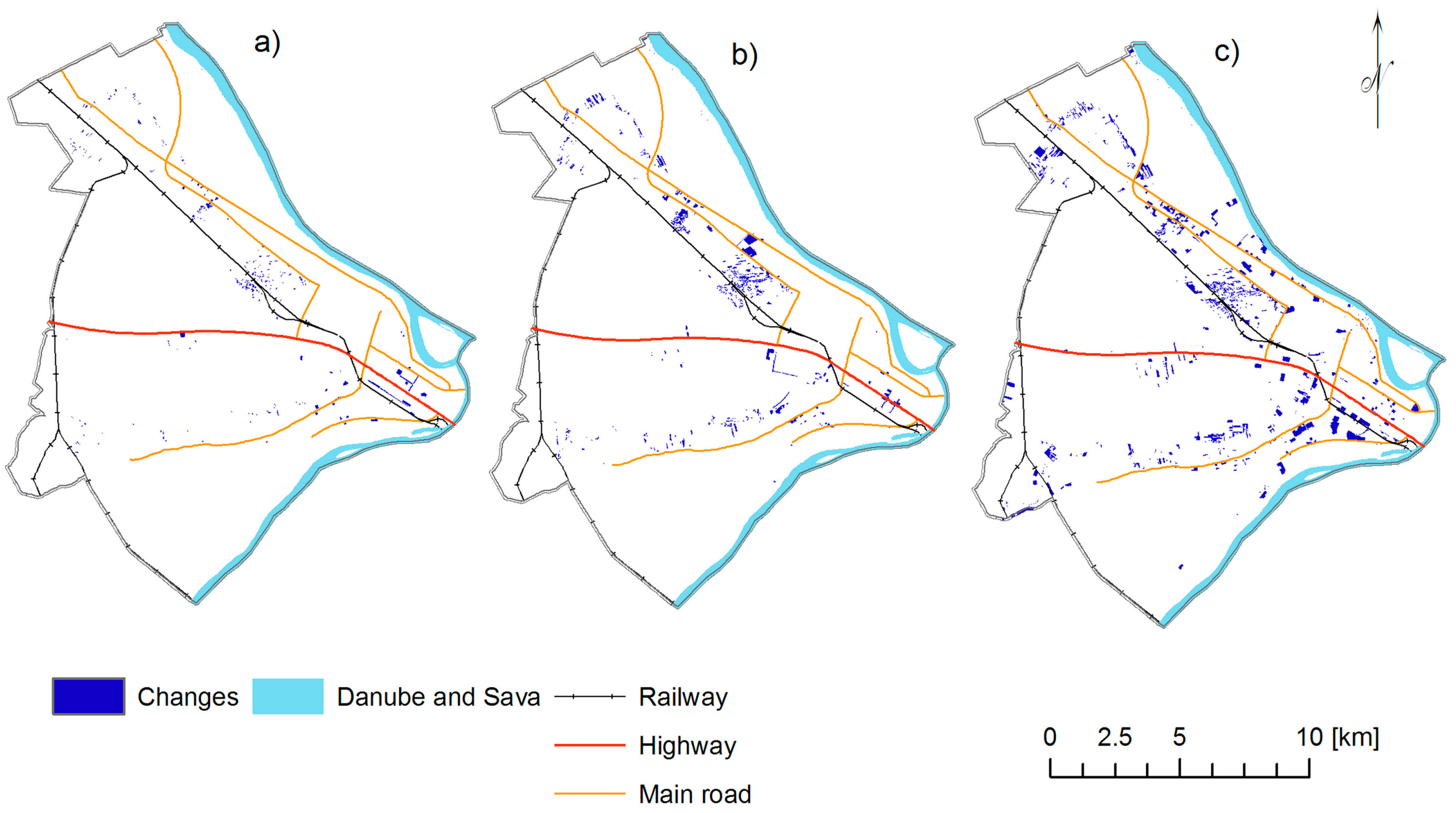
The proposed models for short-term land use forecasting were built and assessed according to the five steps method, as described in Section 2.3. Since there was only a 4% change in the study area for the 10-year time interval 2001–2011 (Figure 2), two balanced data sets, S3–7 for training and S7–11 for testing, were sampled from the corresponding initial sets and the cells were represented according to the Section 2.3, step 1, using time points 2001 (only previous land use class), 2003, 2007 and 2011 (Table 2).
In order to assess the importance of each considered attribute, the IG ranking method was applied on the training set S3–7. The obtained attribute rankings are shown in Table 3. The highest ranked attribute represented the previous land use class (year 2001), while the present land use class was the second ranked attribute with an almost identical IG score. The next ranked was the most frequent land use class in the neighborhood reflecting the importance of the influence of nearby cells. Other informative attributes were related to the proximity of the city center and the distance to the highways. The lowest ranked were related to the attributes that did not change at all, or only by a very small amount, during the observed time interval, such as distances to the river and railway, or the number of inhabitants per cell. The obtained attribute ranking is meaningful for the urban planning purposes, except for the attribute mun_code. The municipality code attribute (only three distinct values) is ranked much lower when compared with an urban expert’s point of view, in respect that the study area municipalities are very different in the sense of urban growth. The reason for the lower ranking of that attribute could be that IG is biased towards choosing attributes with a large number of values.
In order to examine the effects of selecting the top n informative attributes by IG to the classification performance, a recursive attribute elimination method was applied. The lowest-ranked attribute was removed from the training and test data set in each iteration until all of the attributes have been removed. The obtained performance curves for all three ML techniques are presented in Figure 3.
Generally, the overall model performance suggest that all three ML techniques are capable to effectively model short term land use changes with slight differences. Even with a small number of used attributes, ML based model can derive outcomes, with high values of weighted AUC (Figure 3). By comparing the obtained performance curves, it can be concluded that SVM and NN have a greater power of generalization when compared to DT. Values of weighted AUC indicate that the accuracy of the tested ML techniques declined abruptly when using less than five first-ranked attributes. Furthermore, it can be noted that the elimination of certain attributes improved the classification capability as a result of reduced model complexity, while retaining enough information about the phenomenon and the same number of teaching examples. This indicates that the initial selection of attributes that are given in Table 1 was justified for the study area and included real, informative predictors for LUC. Values of weighted average TPrate indicate that the DT method is approximately 5% less efficient in classification of predicted land use class when compared with the two other used techniques. Furthermore, weighted average TPrate values declined sharply for all three ML techniques when using four and less first-ranked attributes by IG, while weighted average FPrate values increased. The recursive attribute elimination should be stopped when the performance measures TPrate/FPrate start to drop/increase significantly.
An in-depth analysis of the results is realized by using the three maps comparison method, with a separate investigation of simulation outcomes of persistent and changed cells (Figure 4). This method allows for more insight into the model’s performance and their mutual differences are more evident in comparison to weighted averages AUC, TPrate, and FPrate. The number of changed cells that are simulated correctly and that are simulated as persistent (Figure 4a,b) also indicate that the accuracy of the tested ML techniques declines abruptly when using less than five first-ranked attributes. The agreement between simulated changed and in reality changed cells (Figure 4a) suggests that SVM had a better ability to learn changes in a land use class when compared to NN and DT. DT favored the persistence of the land use class (Figure 4c,e). When comparing the disagreements for the changed cells (Figure 4b,d), it can be concluded that most of them were related to cells that were changed in reality, whereas the model simulated them as persistent. All of the ML techniques were capable of learning the concept of unchanging cells.
Taking into account all of the measures, the best performing models were built using the first nine ranked attributes for DT and SVM, and the first 11 ranked attributes for NN. A detailed per-class insight into the behavior of the best performing models is given in Table 4.
DT is less capable of predicting the Commercial land use class in comparison to the other two techniques. Concerning the Infrastructure class, none of the Infrastructure objects have been built from 2001 to 2011. Therefore, DT and SVM, as opposed to NN, successfully “learned” that this class did not change. The small amount of changes in the Wetland class during the observed time interval was caused by the start of construction of the bridge over the Sava. All of the ML techniques registered those changes during the learning process. When initially reducing from 13 to nine classes, the existing Not built land use class was transformed into the Green area or Agriculture classes that were based on the actual conditions detected on the orthophoto maps. Additionally, the Green area class contains areas that are used for several different purposes (cemeteries, parks, recreation, etc.). Therefore, the ML techniques had difficulties in learning related transition rules.
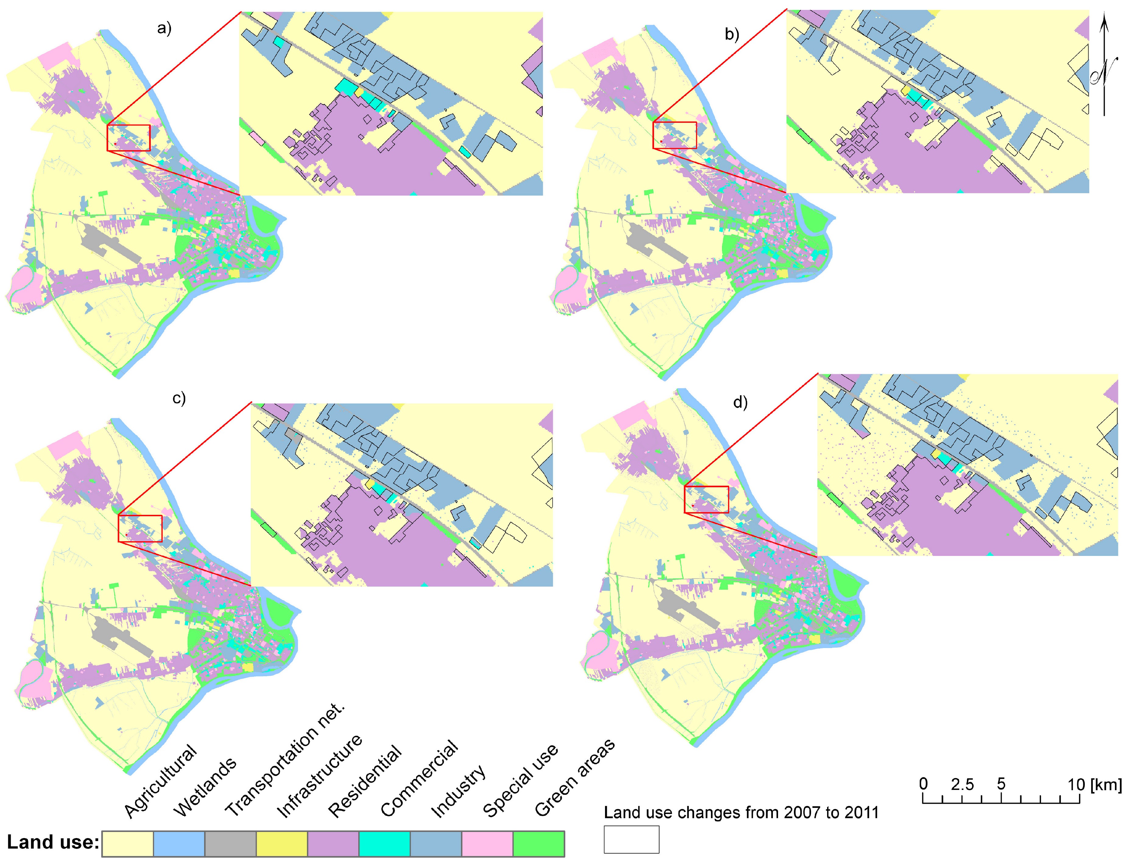
Figure 5 shows the actual and forecasted LUCs from 2007 to 2011 for the entire study area. Maps were generated by the best performing models trained on the balanced set S3–7 after the removal of the less informative attributes.
Based on the interpretation of the generated maps by urban experts, it was concluded that all three models successfully forecasted the LUCs from 2007 to 2011 in three Belgrade municipalities. The SVM and NN models showed slightly better performance than DT. However, DT has a distinct advantage to be used in cases when experts require insight into the model internals since if-then rules can easily be generated. In addition, DT is faster to train than SVM and NN. However, the calibration process of a DT model is less complex when compared with the two other ML techniques, which require the optimization of the pairs of relevant algorithm parameters. Nevertheless, the SVM and NN have a better capability to provide a good generalization of land use changes. Furthermore, the SVM technique is less prone to overfitting when compared to NN.
5. Conclusions
This research examined LUC models that were based on ML techniques in an urban environment with nine land use classes. The obtained results demonstarted that ML models are capable to learn the transition rules in a supervised manner by utilizing the spatial data and land use classes at time point t – 1 and land use classes at time point t. Assuming the existence of an unknown transition function that retains similar properties over the short period of time, two to four years, the model is capable of forecasting land use classes at time point t + 1 from the spatial data that is describing the area at time point t. The ML-based models are capable to forecast the LUC and could be a valuable decision support tool for municipal services that require information related to land-use when experts are not available. Furthermore, experts can benefit from such ML models in a way to better understand relations that are hidden in the data and to complement other expert knowledge approaches.
A comparison was made between three common ML techniques (DT, NN, SVM) when building LUC models from the historic spatial and land use data. The SVM method was the best to forecast the land use changes, while the DT method was capable to learn the concept of no change better than other two. Finally, the DT method can be perceived as easiest to interpret over techniques such as NN and SVM.
One of the objectives of the research was to find the appropriate data representation for learning. Initial representation included common spatial urban indicators (present land use class, distances to city center, highways, roads, etc.) that were augmented with neighboring information about land use classes and history information about previous land uses at each cell in the grid. A detailed analysis using the IG ranking method was done to find the most informative attributes that are related to LUC in the study area. It was found that the reduced number of attributes produced less complex models with a better predictive performance.
Acknowledgments
This research study was supported by the Ministry of Education, Science and Technological Development, Republic of Serbia (Project No. III 47014) awarded to the first three authors and by the Natural Sciences and Engineering Research Council (NSERC) of Canada Discovery Grant awarded to the fourth author. The authors thank the Urban Planning Institute of Belgrade, MapSoft d.o.o. Geo Info Strategies for providing some of the datasets used, and the West Grid, Compute Canada infrastructure for facilitating the computing-intensive data processing. We are thankful to three anonymous reviewers for the detailed and valuable feedback.
Author Contributions
All authors worked equally on the research conceptualization, design and analysis of obtained results. Mileva Samardžić-Petrović was involved in data collection and processing, implementation and execution of the experiments within the various software and generation of results. Mileva Samardžić-Petrović, Branislav Bajat, Miloš Kovačević and Suzana Dragićević participated in the writing of the manuscript, however Mileva Samardžić-Petrović has taken the lead.
Conflicts of Interest
The authors declare no conflict of interest.
References
- Agarwal, C.; Green, G.M.; Grove, J.M.; Evans, T.P.; Schweik, C.M. A Review and Assessment of Land-Use Change Models: Dynamics of Space, Time, and Human Choice; General Technical Report NE 297; U.S. Department of Agriculture, Forest Service, Northeastern Research Station: Newton Square, PA, USA, 2002. [CrossRef]
- Verburg, P.; Schot, P.; Dijst, M.; Veldkamp, A. Land use change modelling: Current practice and research priorities. GeoJournal 2004, 61, 309–324. [Google Scholar] [CrossRef]
- Turner, B.L.; Lambin, E.F.; Reenberg, A. The emergence of land change science for global environmental change and sustainability. Proc. Natl. Acad. Sci. USA 2007, 104, 20666–20671. [Google Scholar] [CrossRef] [PubMed]
- Schneider, L.C.; Pontius, R.G. Modeling land-use change in the Ipswich watershed, Massachusetts, USA. Agric. Ecosyst. Environ. 2001, 85, 83–94. [Google Scholar] [CrossRef]
- Verburg, P.H.; De Koning, G.H.J.; Kok, K.; Veldkamp, A.; Bouma, J. A spatial explicit allocation procedure for modelling the pattern of land use change based upon actual land use. Ecol. Model. 1999, 116, 45–61. [Google Scholar] [CrossRef]
- Hu, Z.; Lo, C.P. Modeling urban growth in Atlanta using logistic regression. Comput. Environ. Urban Syst. 2007, 31, 667–688. [Google Scholar] [CrossRef]
- Muller, M.R.; Middleton, J. A Markov model of land-use change dynamics in the Niagara Region, Ontario, Canada. Landsc. Ecol. 1994, 9, 151–157. [Google Scholar] [CrossRef]
- Lopez, E.; Bocco, G.; Mendoza, M.; Duhau, E. Predicting land-cover and land-use change in the urban fringe: A case in Morelia city, Mexico. Landsc. Urban Plan. 2001, 55, 271–285. [Google Scholar] [CrossRef]
- White, R.; Engelen, G.; Uljee, I. The use of constrained cellular automata for high-resolution modelling of urban land-use dynamics. Environ. Plan. B Plan. Des. 1997, 24, 323–343. [Google Scholar] [CrossRef]
- Van Vliet, J.; White, R.; Dragicevic, S. Modeling urban growth using a variable grid cellular automaton. Comput. Environ. Urban Syst. 2009, 33, 35–43. [Google Scholar] [CrossRef]
- Yao, Y.; Li, J.; Zhang, X.; Duan, P.; Li, S.; Xu, Q. Investigation on the Expansion of Urban Construction Land Use Based on the CART-CA Model. ISPRS Int. J. Geo-Inf. 2017, 6, 149. [Google Scholar] [CrossRef]
- Brown, D.G.; Page, S.; Riolo, R.; Zellner, M.; Rand, W. Path dependence and the validation of agent-based spatial models of land use. Int. J. Geogr. Inf. Sci. 2005, 19, 153–174. [Google Scholar] [CrossRef]
- Groeneveld, J.; Müller, B.; Buchmann, C.M.; Dressler, G.; Guo, C.; Hase, N.; Hoffmann, F.; John, F.; Klassert, C.; Lauf, T.; et al. Theoretical foundations of human decision-making in agent-based land use models—A review. Environ. Model. Softw. 2017, 87, 39–48. [Google Scholar] [CrossRef]
- Tayyebi, A.; Pijanowski, B.C. Modeling multiple land use changes using ANN, CART and MARS: Comparing tradeoffs in goodness of fit and explanatory power of data mining tools. Int. J. Appl. Earth. Obs. 2014, 28, 102–116. [Google Scholar] [CrossRef]
- Kamusoko, C.; Gamba, J. Simulating Urban Growth Using a Random Forest-Cellular Automata (RF-CA) Model. ISPRS Int. J. Geoinf. 2015, 4, 447–470. [Google Scholar] [CrossRef]
- Kjærulff, U.B.; Madsen, A.L. Bayesian Networks and Influence Diagrams: A Guide to Construction and Analysis; Springer: New York, NY, USA, 2008; ISBN 978-0-38-774100-0. [Google Scholar]
- Tafazzoli Moghaddam, E. Data-driven Process Monitoring and Diagnosis with Support Vector Data Description. Unpulished Master’s Thesis, Simon Fraser University, Burnaby, BC, Canada, 2011. [Google Scholar]
- Brown, D.G.; Band, L.E.; Green, K.O.; Irwin, E.G.; Jain, A.; Lambin, E.F.; Pontius, R.G., Jr.; Seto, K.C.; Turner, B.L.I.; Verburg, P.H. Advancing Land Change Modeling: Opportunities and Research Requirements; National Academies Press: Washington, DC, USA, 2014; ISBN 0309288363. [Google Scholar]
- Solomatine, D.P.; Ostfeld, A. Data-driven modelling: Some past experiences and new approaches. J. Hydroinform. 2008, 10, 3–22. [Google Scholar] [CrossRef]
- Naghibi, S.A.; Pourghasemi, H.R.; Dixon, B. GIS-based groundwater potential mapping using boosted regression tree, classification and regression tree, and random forest machine learning models in Iran. Environ. Monit. Assess. 2016, 188, 1–27. [Google Scholar] [CrossRef] [PubMed]
- Marjanović, M.; Kovačević, M.; Bajat, B.; Voženilek, V. Landslide susceptibility assessment using SVM machine learning algorithm. Eng. Geol. 2011, 123, 225–234. [Google Scholar] [CrossRef]
- Pradhan, B. A comparative study on the predictive ability of the decision tree, support vector machine and neuro-fuzzy models in landslide susceptibility mapping using GIS. Comput. Geosci.-UK 2013, 51, 350–365. [Google Scholar] [CrossRef] [Green Version]
- Dickson, M.E.; Perry, G.L.W. Identifying the controls on coastal cliff landslides using machine-learning approaches. Environ. Model. Softw. 2016, 76, 117–127. [Google Scholar] [CrossRef]
- Corani, G. Air quality prediction in Milan: feed-forward neural networks, pruned neural networks and lazy learning. Ecol. Model. 2005, 185, 513–529. [Google Scholar] [CrossRef]
- Leuenberger, M.; Kanevski, M. Extreme Learning Machines for spatial environmental data. Comput. Geosci.-UK 2015, 85, 64–73. [Google Scholar] [CrossRef]
- Pourtaghi, Z.S.; Pourghasemi, H.R.; Aretano, R.; Semeraro, T. Investigation of general indicators influencing on forest fire and its susceptibility modeling using different data mining techniques. Ecol. Indic. 2016, 64, 72–84. [Google Scholar] [CrossRef]
- Bischof, H.; Schneider, W.; Pinz, A.J. Multispectral classification of Landsat-images using neural networks. IEEE Trans. Geosci. Remote Sens. 1992, 30, 482–490. [Google Scholar] [CrossRef]
- Friedl, M.A.; Brodley, C.E. Decision tree classification of land cover from remotely sensed data. Remote Sens. Environ. 1997, 61, 399–409. [Google Scholar] [CrossRef]
- Schwert, B.; Rogan, J.; Giner, N.M.; Ogneva-Himmelberger, Y.; Blanchard, S.D.; Woodcock, C. A comparison of support vector machines and manual change detection for land-cover map updating in Massachusetts, USA. Remote Sens. Lett. 2013, 4, 882–890. [Google Scholar] [CrossRef]
- Goetz, J.N.; Brenning, A.; Petschko, H.; Leopold, P. Evaluating machine learning and statistical prediction techniques for landslide susceptibility modeling. Comput. Geosci.-UK 2015, 81, 1–11. [Google Scholar] [CrossRef]
- Qian, Y.G.; Zhou, W.Q.; Yan, J.L.; Li, W.F.; Han, L.J. Comparing Machine Learning Classifiers for Object-Based Land Cover Classification Using Very High Resolution Imagery. Remote Sens. 2015, 7, 153–168. [Google Scholar] [CrossRef]
- Rodriguez-Galiano, V.; Sanchez-Castillo, M.; Chica-Olmo, M.; Chica-Rivas, M. Machine learning predictive models for mineral prospectivity: An evaluation of neural networks, random forest, regression trees and support vector machines. Ore Geol. Rev. 2015, 71, 804–818. [Google Scholar] [CrossRef]
- Heung, B.; Ho, H.C.; Zhang, J.; Knudby, A.; Bulmer, C.E.; Schmidt, M.G. An overview and comparison of machine-learning techniques for classification purposes in digital soil mapping. Geoderma 2016, 265, 62–77. [Google Scholar] [CrossRef]
- Hong, H.; Pourghasemi, H.R.; Pourtaghi, Z.S. Landslide susceptibility assessment in Lianhua County (China): A comparison between a random forest data mining technique and bivariate and multivariate statistical models. Geomorphology 2016, 259, 105–118. [Google Scholar] [CrossRef]
- Johnson, M.D.; Hsieh, W.W.; Cannon, A.J.; Davidson, A.; Bédard, F. Crop yield forecasting on the Canadian Prairies by remotely sensed vegetation indices and machine learning methods. Agric. For. Meteorol. 2016, 218, 74–84. [Google Scholar] [CrossRef]
- Meyer, H.; Kühnlein, M.; Appelhans, T.; Nauss, T. Comparison of four machine learning algorithms for their applicability in satellite-based optical rainfall retrievals. Atmos. Res. 2016, 169(Part B), 424–433. [Google Scholar] [CrossRef]
- Yeh, A.G.O.; Li, X. Simulation of development alternatives using neural networks, cellular automata, and GIS for urban planning. Photogramm. Eng. Remote Sens. 2003, 69, 1043–1052. [Google Scholar] [CrossRef]
- Almeida, C.M.; Gleriani, J.M.; Castejon, E.F.; Soares, B.S. Using neural networks and cellular automata for modelling intra-urban land-use dynamics. Int. J. Geogr. Inf. Sci. 2008, 22, 943–963. [Google Scholar] [CrossRef]
- Pijanowski, B.C.; Brown, D.G.; Shellito, B.A.; Manik, G.A. Using neural networks and GIS to forecast land use changes: A land transformation model. Comput. Environ. Urban Syst. 2002, 26, 553–575. [Google Scholar] [CrossRef]
- Liu, W.; Seto, K.; Sun, Z.; Tian, Y. Urban land use prediction model with spatiotemporal data mining and GIS. In Urban Remote Sensing; Weng, Q., Quattrochi, D.A., Eds.; CRC Press, Taylor and Francis Group: Boca Raton, FL, USA, 2007; pp. 165–178. ISBN 1420008803. [Google Scholar]
- Li, X.; Yeh, A.G.O. Data mining of cellular automata’s transition rules. Int. J. Geogr. Inf. Sci. 2004, 18, 723–744. [Google Scholar] [CrossRef]
- Yang, Q.; Li, X.; Shi, X. Cellular automata for simulating land use changes based on support vector machines. Comput. Geosci.-UK 2008, 34, 592–602. [Google Scholar] [CrossRef]
- Okwuashi, O.; McConchie, J.; Nwilo, P.; Isong, M.; Eyoh, A.; Nwanekezie, O. Predicting future land use change using support vector machine based GIS cellular automata: A case of Lagos, Nigeria. J. Sustain. Dev. 2012, 5, 132–139. [Google Scholar] [CrossRef]
- Huang, B.; Xie, C.; Tay, R. Support Vector Machines for urban growth modeling. Geoinformatica 2010, 14, 83–99. [Google Scholar] [CrossRef]
- Gong, Z.; Thill, J.C.; Liu, W. ART-P-MAP Neural Networks Modeling of Land-Use Change: Accounting for Spatial Heterogeneity and Uncertainty. Geogr. Anal. 2015, 47, 376–409. [Google Scholar] [CrossRef]
- Qiang, Y.; Lam, N.S. Modeling land use and land cover changes in a vulnerable coastal region using artificial neural networks and cellular automata. Environ. Monit. Assess. 2015, 187, 1–16. [Google Scholar] [CrossRef] [PubMed]
- Liu, H.; Motoda, H. Feature Selection for Knowledge Discovery and Data Mining; Springer: New York, NY, USA, 1998; ISBN 978-0-79-238198-3. [Google Scholar]
- Kim, Y.; Street, W.N.; Menczer, F. Feature selection in data mining. In Data Mining: Opportunities and Challenges; Wang, J., Ed.; IRM Press (an imprint of Idea Group Inc.): London UK, 2003; Volume 3, pp. 80–105. ISBN 1591400511. [Google Scholar]
- Samardžić-Petrović, M.; Dragićević, S.; Bajat, B.; Kovačević, M. Exploring the Decision Tree Method for Modelling Urban Land Use Change. Geomatica 2015, 69, 313–325. [Google Scholar] [CrossRef]
- Arango, R.B.; Díaz, I.; Campos, A.; Canas, E.R.; Combarro, E.F. Automatic arable land detection with supervised machine learning. Earth Sci. Inform. 2016, 9, 535–545. [Google Scholar] [CrossRef]
- Bradley, A.P. The use of the area under the roc curve in the evaluation of machine learning algorithms. Pattern Recognit. 1997, 30, 1145–1159. [Google Scholar] [CrossRef]
- Pontius, R.G., Jr.; Peethambaram, S.; Castella, J.C. Comparison of three maps at multiple resolutions: A case study of land change simulation in Cho Don District, Vietnam. Ann. Assoc. Am. Geogr. 2011, 101, 45–62. [Google Scholar] [CrossRef]
- Gahegan, M. On the application of inductive machine learning tools to geographical analysis. Geogr. Anal. 2000, 32, 113–139. [Google Scholar] [CrossRef]
- Samardžić-Petrović, M.; Dragićević, S.; Kovačević, M.; Bajat, B. Modeling Urban Land Use Changes Using Support Vector Machines. Trans. GIS 2016, 20, 718–734. [Google Scholar] [CrossRef]
- Shannon, C.E. A Mathematical Theory of Communication. Bell Syst. Tech. J. 1948, 27, 379–423. [Google Scholar] [CrossRef]
- Witten, I.H.; Frank, E.; Hall, M.A. Data Mining: Practical Machine Learning Tools and Techniques, 3rd ed.; Morgan Kaufmann Publishers Inc.: San Francisco, CA, USA, 2011; ISBN 978-0-12-374856-0. [Google Scholar]
- Fawcett, T. An introduction to ROC analysis. Pattern Recognit. Lett. 2006, 27, 861–874. [Google Scholar] [CrossRef]
- Rokach, L.; Maimon, O. Data Mining with Decision Trees: Theory and Applications, 2nd ed.; World Scientific: Singapore, 2014; ISBN 9814590096. [Google Scholar]
- Breiman, L.; Friedman, J.; Olshen, R.; Stone, C. Classification and Regression Trees; Chapman and Hall/CRC, Taylor and Francis Groupe: Boca Raton, FL, USA, 1984; ISBN 0412048418. [Google Scholar]
- Quinlan, J.R. Induction of decision trees. Mach. Learn. 1986, 1, 81–106. [Google Scholar] [CrossRef]
- Quinlan, J.R. C4.5: Programs for Machine Learning; Morgan Kaufmann Publishers: San Mateo, CA, USA, 1993; ISBN 978-0-08-050058-4. [Google Scholar]
- Rosenblatt, F. The perceptron: A probabilistic model for information storage and organization in the brain. Psychol. Rev. 1958, 65, 386–408. [Google Scholar] [CrossRef] [PubMed]
- Kohonen, T. Self-organized formation of topologically correct feature maps. Biol. Cybern. 1982, 43, 59–69. [Google Scholar] [CrossRef]
- Broomhead, D.S.; Lowe, D. Radial Basis Functions, Multi-Variable Functional Interpolation and Adaptive Networks; Royal Signals and Radar Establishment Malvern: Malvern, UK, 1988; Available online: http://www.dtic.mil/docs/citations/ADA196234 (accessed on 27 November 2017).
- Rumelhart, D.E.; Hinton, G.E.; Williams, R.J. Learning representations by back-propagating errors. Nature 1986, 323, 533–536. [Google Scholar] [CrossRef]
- Jain, A.K.; Mao, J.C.; Mohiuddin, K.M. Artificial neural networks: A tutorial. Computer 1996, 29, 31–44. [Google Scholar] [CrossRef]
- Cristianini, N.; Shawe-Taylor, J. An Introduction to Support Vector Machines and Other Kernel-Based Learning Methods; Cambridge University Press: Cambridge, New York, NY, USA, 2000; ISBN 0521780195. [Google Scholar]
- Vapnik, V.N. The Nature of Statistical Learning Theory, 2nd ed.; Springer: New York, NY, USA, 2000; ISBN 978-1-44-193160-3. [Google Scholar]
- Belousov, A.I.; Verzakov, S.A.; Von Frese, J. Applicational aspects of support vector machines. J. Chemom. 2002, 16, 482–489. [Google Scholar] [CrossRef]
- Abe, S. Support Vector Machines for Pattern Classification, 2nd ed.; Springer: London, UK; New York, NY, USA, 2010; ISBN 978-1-84-996097-7. [Google Scholar]
- Hall, M.; Frank, E.; Holmes, G.; Pfahringer, B.; Reutemann, P.; Witten, I.H. The WEKA data mining software: An update. SIGKDD Explor. 2009, 11, 10–18. [Google Scholar] [CrossRef]
- Weka (2016) Weka 3: Data Mining Software in Java. Machine Learning Group at the University of Waikato: New Zealand. Available online: https://www.cs.waikato.ac.nz/ml/weka/ (accessed on 27 November 2017).
- URBEL, Urban Planning Institute of Belgrade. The Master Plan of Belgrade 2021. Official Gazette of the City of Belgrade 27. 2003. Available online: http://www.urbel.com/home.aspx?ID=uzb_Home&LN=ENG (accessed on 7 March 2014).
- Bajat, B.; Krunić, N.; Samardžić-Petrović, M.; Kilibarda, M. Dasymetric modelling of population dynamics in urban areas. Geod. Vestn. 2013, 57, 777–792. [Google Scholar] [CrossRef]
- Conrad, O.; Bechtel, B.; Bock, M.; Dietrich, H.; Fischer, E.; Gerlitz, L.; Wehberg, J.; Wichmann, V.; Böhner, J. System for Automated Geoscientific Analyses (SAGA) v. 2.1.4. Geosci. Model Dev. 2015, 8, 1991–2007. [Google Scholar] [CrossRef]
- ESRI. Version ArcGIS Desktop: Release 10; Environmental Systems Research Institute: Redlands, CA, USA, 2011. [Google Scholar]
Figure 1.
Study area: Municipalities Zemun, New Belgrade, and Surčin from Belgrade metropolitan area, Republic of Serbia.
Figure 1.
Study area: Municipalities Zemun, New Belgrade, and Surčin from Belgrade metropolitan area, Republic of Serbia.

Figure 2.
Land-use changes for the following time intervals: (a) 2001–2003, (b) 2003–2007, and (c) 2007–2011.
Figure 2.
Land-use changes for the following time intervals: (a) 2001–2003, (b) 2003–2007, and (c) 2007–2011.

Figure 3.
Effectiveness of the attribute selection when applied to building models based on weighted average of: (a) Area Under Receiver Operating Characteristic Curve (AUC); (b) True Positive rate (TPrate); (c) False Positive rate (FPrate).
Figure 3.
Effectiveness of the attribute selection when applied to building models based on weighted average of: (a) Area Under Receiver Operating Characteristic Curve (AUC); (b) True Positive rate (TPrate); (c) False Positive rate (FPrate).
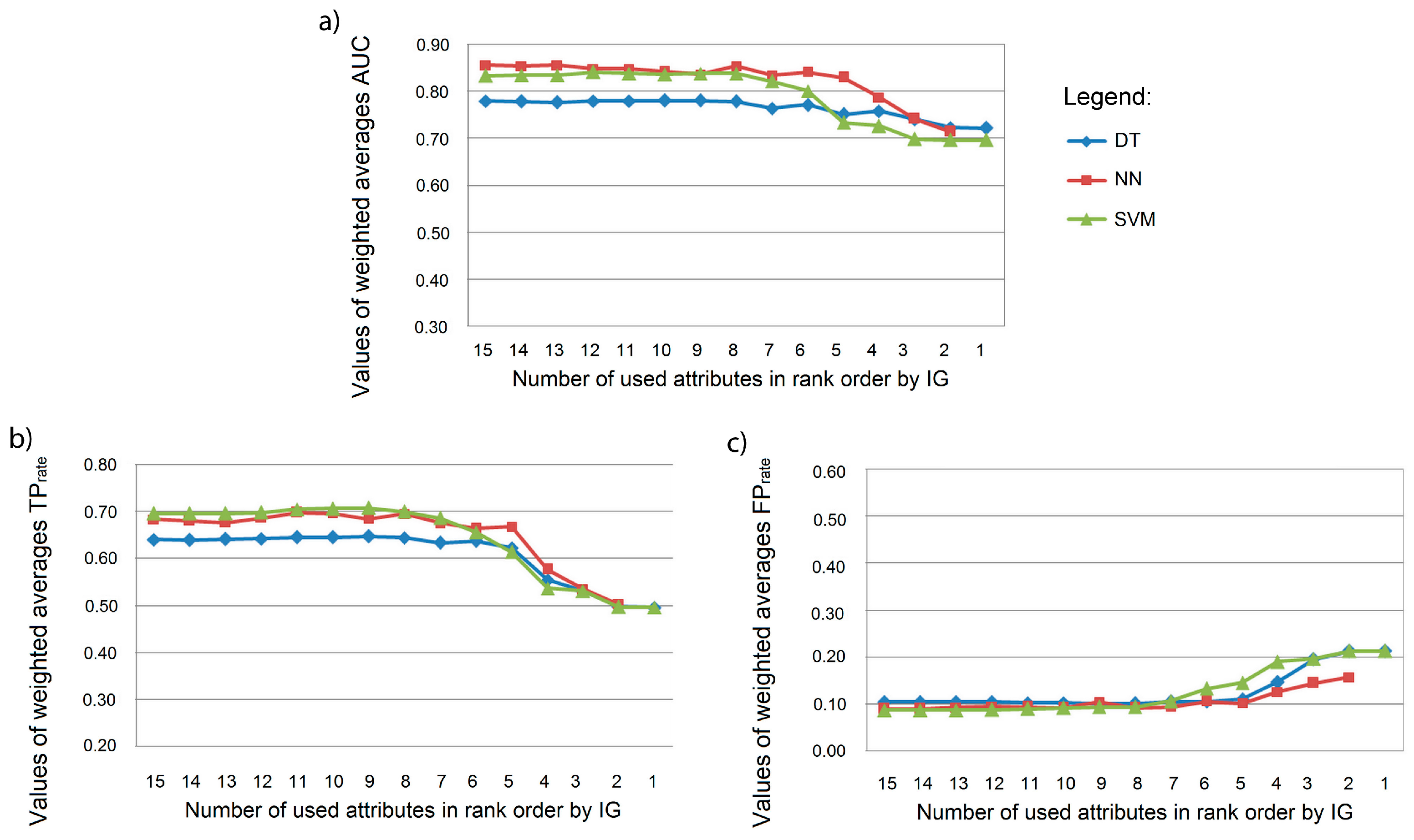
Figure 4.
Effectiveness of the attribute selection when applied to building models based on three maps comparison methods: (a) Number of changed cells simulated correctly; (b) Number of changed cells simulated as persistent; (c) Number of persistent cells simulated correctly; (d) Number of changed cells simulated as change to wrong category; (e) Number of persistent cells simulated as change.
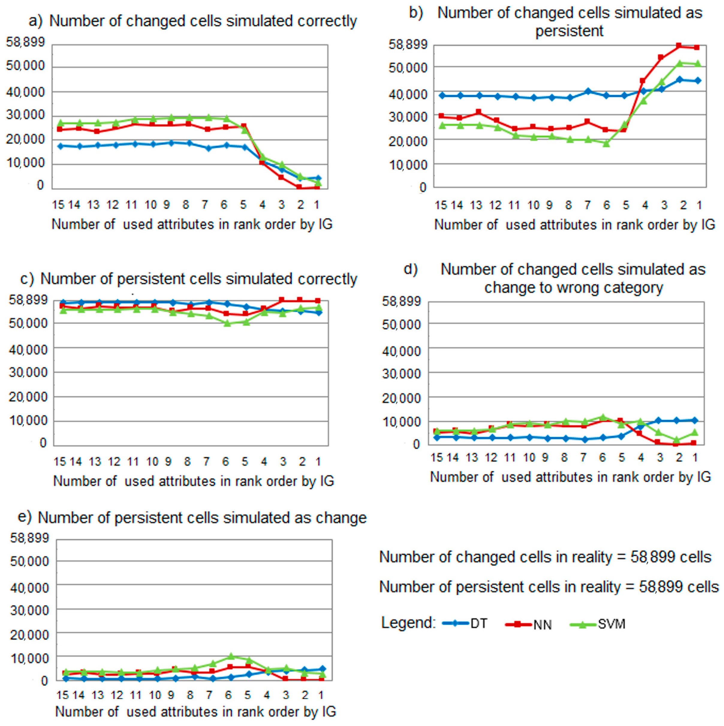
Figure 5.
Generated maps for best performing models for year 2011 (a) Actual land-use and forecasts obtained with (b) Decision Trees (DT), (c) Neural Networks (NN), and (d) Support Vector Machines (SVM).
Figure 5.
Generated maps for best performing models for year 2011 (a) Actual land-use and forecasts obtained with (b) Decision Trees (DT), (c) Neural Networks (NN), and (d) Support Vector Machines (SVM).


Table 1.
List of attributes used for modeling land-use change in the study area.
| Attribute Label | Attribute Description |
|---|---|
| x1 | Municipality code (mun_code) |
| x2 | Distance to city centre (dcitycentre) |
| x3 | Distance to municipality centre (dmuncentre) |
| x4 | Distance to rivers (driver) |
| x5 | Distance to green areas greater than 100 × 100 m (dgreen) |
| x6 | Distance to railway lines (drail) |
| x7 | Distance to highway (dhighway) |
| x8 | Distance to main road (droad) |
| x9 | Distance to the street of category I (dstreetI) |
| x10 | Distance to the street of category II (dstreetII) |
| x11 | Number of inhabitants (no_inhabitants) |
| x12 | Land use class (LU_class) |
| x13 | Most frequent land use class in Moore neighbourhood 7 × 7 (mf_LU_class) |
| x14 | Second most frequent land use class in Moore neighbourhood 7 × 7 (smf_LU_class) |
| x15 | Previous land use class (prev_LU_class) |
Table 2.
Description of data sets used in the experiments.
| Data Set | Attributes from | Class Label from | Number of Cells |
|---|---|---|---|
| S3–7 | 2001, 2003 | 2007 | 51,358 |
| S7–11 | 2003, 2007 | 2011 | 117,798 |
Table 3.
Top ranked attributes based on the Info Gain (IG) method.
| Attribute Rank | Information Gain | Attribute |
|---|---|---|
| 1 | 0.8159 | prev_LU_class |
| 2 | 0.8073 | LU_class |
| 3 | 0.7361 | mf_LU_class |
| 4 | 0.5593 | dcitycentre |
| 5 | 0.4860 | dhighway |
| 6 | 0.4789 | dgreen |
| 7 | 0.4517 | dstreetI |
| 8 | 0.3699 | smf_LU_class |
| 9 | 0.3591 | droad |
| 10 | 0.3538 | dstreetII |
| 11 | 0.3406 | dmuncentre |
| 12 | 0.2545 | drail |
| 13 | 0.2014 | mun_code |
| 14 | 0.0832 | driver |
| 15 | 0.0831 | no_inhabitants |
Table 4.
Effectiveness of the attribute selection when applied to building models based on three maps comparison methods.
Table 4.
Effectiveness of the attribute selection when applied to building models based on three maps comparison methods.
| Land Use Class | ||||||||||
|---|---|---|---|---|---|---|---|---|---|---|
| Agricultural | Wetlands | Trans.net. | Infrastructure | Residential | Commercial | Industr. | Special Use | Green Area | ||
| N 1 in reality | 36,823 | 48 | 165 | 0 | 3698 | 59 | 4237 | 275 | 13,594 | |
| M 2 in reality | 33,530 | 2905 | 2409 | 264 | 9461 | 823 | 2688 | 2775 | 4468 | |
| Measure | ML | |||||||||
| AUC | DT | 0.88 | 0.99 | 0.82 | 1.00 | 0.78 | 0.55 | 0.71 | 0.79 | 0.74 |
| NN | 0.93 | 1.00 | 0.91 | 1.00 | 0.85 | 0.68 | 0.84 | 0.79 | 0.65 | |
| SVM | 0.91 | 0.99 | 0.88 | 1.00 | 0.80 | 0.69 | 0.84 | 0.90 | 0.79 | |
| TPrate | DT | 0.94 | 0.99 | 0.65 | 1.00 | 0.62 | 0.10 | 0.41 | 0.58 | 0.57 |
| NN | 0.92 | 0.97 | 0.64 | 0.99 | 0.72 | 0.34 | 0.52 | 0.58 | 0.45 | |
| SVM | 0.91 | 0.99 | 0.67 | 1.00 | 0.70 | 0.29 | 0.57 | 0.58 | 0.33 | |
| FPrate | DT | 0.20 | 0.00 | 0.01 | 0.00 | 0.09 | 0.01 | 0.05 | 0.00 | 0.10 |
| NN | 0.14 | 0.00 | 0.02 | 0.00 | 0.13 | 0.03 | 0.05 | 0.00 | 0.03 | |
| SVM | 0.14 | 0.00 | 0.01 | 0.00 | 0.15 | 0.03 | 0.06 | 0.00 | 0.03 | |
| N simulated correctly | DT | 16,990 | 10 | 32 | 0 | 569 | 3 | 157 | 43 | 1512 |
| NN | 21,965 | 12 | 45 | 0 | 1508 | 13 | 348 | 79 | 4521 | |
| SVM | 23,697 | 25 | 72 | 0 | 1873 | 19 | 578 | 102 | 5087 | |
| M simulated correctly | DT | 32,504 | 2481 | 2380 | 264 | 9400 | 802 | 2679 | 2769 | 4277 |
| NN | 30,797 | 2481 | 2262 | 264 | 9445 | 770 | 2660 | 2772 | 2489 | |
| SVM | 30,564 | 2478 | 2355 | 264 | 9429 | 758 | 2609 | 2746 | 3306 | |
| NS 3 change to wrong class | DT | 1508 | 0 | 25 | 0 | 34 | 10 | 65 | 16 | 1136 |
| NN | 2912 | 0 | 32 | 0 | 54 | 14 | 2 | 3 | 5491 | |
| SVM | 2680 | 0 | 39 | 0 | 24 | 13 | 258 | 34 | 5272 | |
| NS persistent | DT | 18,325 | 38 | 108 | 0 | 3095 | 46 | 4015 | 216 | 10,946 |
| NN | 11,946 | 36 | 88 | 0 | 2136 | 32 | 3887 | 193 | 3582 | |
| SVM | 10,446 | 23 | 54 | 0 | 1801 | 27 | 3401 | 139 | 3235 | |
| MS 4 change | DT | 1026 | 0 | 29 | 0 | 61 | 21 | 9 | 6 | 191 |
| NN | 2733 | 0 | 147 | 0 | 16 | 53 | 28 | 3 | 1979 | |
| SVM | 2966 | 3 | 54 | 0 | 32 | 65 | 79 | 29 | 1162 | |
1 N-number of changed cells; 2 M-number of persistent cells; 3 NS-number of changed cells simulated as; 4 MS-number of persistent cells simulated as.
© 2017 by the authors. Licensee MDPI, Basel, Switzerland. This article is an open access article distributed under the terms and conditions of the Creative Commons Attribution (CC BY) license (http://creativecommons.org/licenses/by/4.0/).
Share and Cite
MDPI and ACS Style
Samardžić-Petrović, M.; Kovačević, M.; Bajat, B.; Dragićević, S. Machine Learning Techniques for Modelling Short Term Land-Use Change. ISPRS Int. J. Geo-Inf. 2017, 6, 387. https://doi.org/10.3390/ijgi6120387
AMA Style
Samardžić-Petrović M, Kovačević M, Bajat B, Dragićević S. Machine Learning Techniques for Modelling Short Term Land-Use Change. ISPRS International Journal of Geo-Information. 2017; 6(12):387. https://doi.org/10.3390/ijgi6120387
Chicago/Turabian StyleSamardžić-Petrović, Mileva, Miloš Kovačević, Branislav Bajat, and Suzana Dragićević. 2017. "Machine Learning Techniques for Modelling Short Term Land-Use Change" ISPRS International Journal of Geo-Information 6, no. 12: 387. https://doi.org/10.3390/ijgi6120387
Note that from the first issue of 2016, this journal uses article numbers instead of page numbers. See further details here.