An Automatic K-Means Clustering Algorithm of GPS Data Combining a Novel Niche Genetic Algorithm with Noise and Density

Abstract

Rapidly growing Global Positioning System (GPS) data plays an important role in trajectory and their applications (e.g., GPS-enabled smart devices). In order to employ K-means to mine the better origins and destinations (OD) behind the GPS data and overcome its shortcomings including slowness of convergence, sensitivity to initial seeds selection, and getting stuck in a local optimum, this paper proposes and focuses on a novel niche genetic algorithm (NGA) with density and noise for K-means clustering (NoiseClust). In NoiseClust, an improved noise method and K-means++ are proposed to produce the initial population and capture higher quality seeds that can automatically determine the proper number of clusters, and also handle the different sizes and shapes of genes. A density-based method is presented to divide the number of niches, with its aim to maintain population diversity. Adaptive probabilities of crossover and mutation are also employed to prevent the convergence to a local optimum. Finally, the centers (the best chromosome) are obtained and then fed into the K-means as initial seeds to generate even higher quality clustering results by allowing the initial seeds to readjust as needed. Experimental results based on taxi GPS data sets demonstrate that NoiseClust has high performance and effectiveness, and easily mine the city’s situations in four taxi GPS data sets.

1. Introduction

Nowadays, with the prevalence of smart Global Positioning System (GPS) devices with positioning ability, a large amount of GPS-based data and trajectories are available. There is a huge amount of hidden information behind location data, which are very useful in providing many services to people such as navigation and recommendation systems based on taxi position, the localization of points of interest, the population migration distribution of a city, land use, and the analysis of traffic flow. The key element to these applications is location (based on GPS), which is required to mine the hidden information and understand the meaning of the trajectories, instead of only considering trajectory as a combination of recorded GPS data points. Therefore, in these application domains, techniques for mining trajectory patterns and frequent trajectory routes are very important [1], and have usually been described by several trajectory patterns, such as origins and destinations (OD) [2,3,4], stops and moves [5,6], moving object [7,8]; furthermore, a great quantity of clustering algorithms have been used to mine these patterns and produce clustering results. For example, the authors of [6] presented an improved DBSCAN (Density-Based Spatial Clustering of Applications with Noise) algorithm to be used for stops clustering in trajectories; the authors in [3] proposed an OD pattern of interested regions based on taxi trajectories; Reference [4] presented a new spatio-temporal queries model that allowed users to visually query taxi trips through OD; a density-based clustering approach was presented in [9] that aimed at mining the topology of stops of a public transport network; a hierarchical clustering algorithm was proposed to first extract visit points from GPS trajectories in [10], then clustered these visit points with the aim to discover personally semantic places; Reference [11] proposed a density-based line-segment trajectories clustering algorithm based on partition and group framework; and [12] presented a mode-based clustering algorithm for trajectories, and an EM (Expectation–Maximization) algorithm was used to determine the cluster memberships.

In general, most of the existing clustering algorithms used in GPS data clustering suffer from their respective drawbacks, which are also deemed to be some of the most difficult and challenging problems in unsupervised machine learning [6,13,14,15]. In fact, clustering is an important data analysis approach and data mining technique that is used for identifying clusters of similar characteristics and dissimilar records in different clusters, and has a wide range of applications including machine learning, social network analysis, and the geosciences. Unfortunately, it is difficult to find the number of natural clusters; moreover, the clustering result is sensitive to the selection of the initial seeds. There are many clustering algorithms (e.g., density-based, partition-based) [14], out of which K-means (partition-based) is a more commonly-used technique—perhaps because of its simplicity and effectiveness—than other clustering algorithms (e.g., density-based, model-based). However, K-means requires a user to provide the number of clusters K as an input [15,16], and may converge to a partition that is significantly inferior or slow compared to the global optimum [17]. Based on this user-defined value of the number of clusters, K-means randomly selects a K number of initial seeds from a given dataset [18]. Namely, K-means is generally very sensitive to the quality of the initial seeds, therefore it is easy to produce poor quality results due to the poor quality of initial seeds [16,19]. Therefore, clustering techniques that are capable of automatically selecting the number of clusters are highly desirable [16]. Another drawback of K-means is that it does not record the quality of clusters obtained in the previous iterations. To improve the performance and enhance the efficiency of the K-means algorithm, several genetic algorithms (GAs) with K-means have been developed in the past few years [20,21,22]. The use of GAs with K-means can help to avoid the minima issues of the K-means [16,20,21,22,23], and can produce better clustering results than the K-means or GA clustering. For example, GenClust [16] can automatically find the appropriate number of clusters and identify the right genes through a novel initial population selection approach. AGCUK (Automatic genetic clustering for unknown K) [22] presented an automatic genetic clustering algorithm for an unknown K to automatically find the number of clusters and provide the proper clustering partition. GAGR (Genetic algorithm with gene rearrangement) [20] proposed a GA-based K-means clustering algorithm with gene rearrangement. GGA (Group genetic algorithm) [21] presented GA-based clustering algorithms with a new grouping method in the initial population. However, these GAs with K-means can lose population diversity due to global optimal problems and weak exploitation capabilities, and the gene size of the chromosomes must be equal in the AGCUK (Automatic genetic clustering for unknown K) and GAGR. In GGA algorithm, the number of clusters require a user input, but gene sizes are not equal.

In this paper, the presented novel clustering algorithm called NoiseClust (niche genetic algorithm (NGA) combining noise and density with K-means) combined a novel NGA with K-means for taxi GPS data clustering, which is used to mine the better OD. Part of NoiseClust includes an improved noise and K-means++ [24,25], which are used to generate the initial population and initial seeds without requiring a user to input the number of clusters, and can also handle the different size and shape of genes. Meanwhile, density-based niche partitioning and sharing-based niche are used to maintain population diversity, capture the global optimal solution, and enhance exploitation capabilities [26,27], meanwhile, adaptive crossover and mutation probabilities are also employed to avoid the local optimum.

NoiseClust can improve the gene rearrangement operation of GenClust [16] by using the cosine similarity between chromosomes before a crossover. The improved method can handle the similarity between chromosomes, and the distance between taxi GPS data points of the crossover operation do not have an equal number of genes. Therefore, the advantage of the improved method is the ease in selecting the best chromosomes in the crossover operation during each iteration, which strengthens the capability of gene rearrangement in the different NGA operations. Prior to this, a novel initial population method with noise and K-means++ is also proposed in NoiseClust, where its aim was to strengthen efficiency and reduce the complexity of the initial population.

Additionally, the NoiseClust technique integrates an improved NGA and K-means to generate higher quality clustering results than GenClust [16]. The NGA consists of two parts: (1) the density estimation is used to divide the number of niches that maintains population diversity; (2) the Pearson similarity [28] between chromosomes is used to replace the distance in the sharing function of niches [29] with the advantage of better stability and diversity of the population than GA (see Section 2.6.2). Our proposed clustering technique overcomes the issues of K-means by using our NGA, which automatically selects the high-quality initial seeds. Namely, the NoiseClust clustering algorithm does not only automatically capture the number of clusters, overcomes the local minima issue and avoids sensitive seed selection for K-means, but also strengthens the diversity of the population and avoids premature convergence.

To verify the performance and effectiveness of NoiseClust, four taxi GPS data sets are used as examples (see Section 2.1), and the experiments compare NoiseClust with GenClust [16] and Genetic algorithm K-means (GAK) [30] on three cluster evaluation criteria: silhouette coefficient (SC) [21], PBM (Pakhira-Bandyopadhyay-Maulik) [31] and SSE (Sum of Squared Errors) [20]. These results indicate that NoiseClust achieves better quality clusters than the GenClust and GAK algorithms. Furthermore, this paper also presents a complexity analysis of NoiseClust in Section 2.10.

Therefore, the main works of the paper are summarized as follows:

• The selection of the initial population combining noise with K-means++.
• An improved gene rearrangement technique using cosine similarity.
• Adaptive probabilities of crossover and mutation are used to prevent the NoiseClust from getting stuck at a local optimal solution.
• A novel niche operation is proposed to maintain population diversity.
• NoiseClust works on four real-world taxi GPS data sets.

The remainder of the paper is organized as follows: Section 2 describes our proposed novel clustering algorithm. Experimental results are presented in Section 3. Finally, Section 4 offers conclusions and future work.

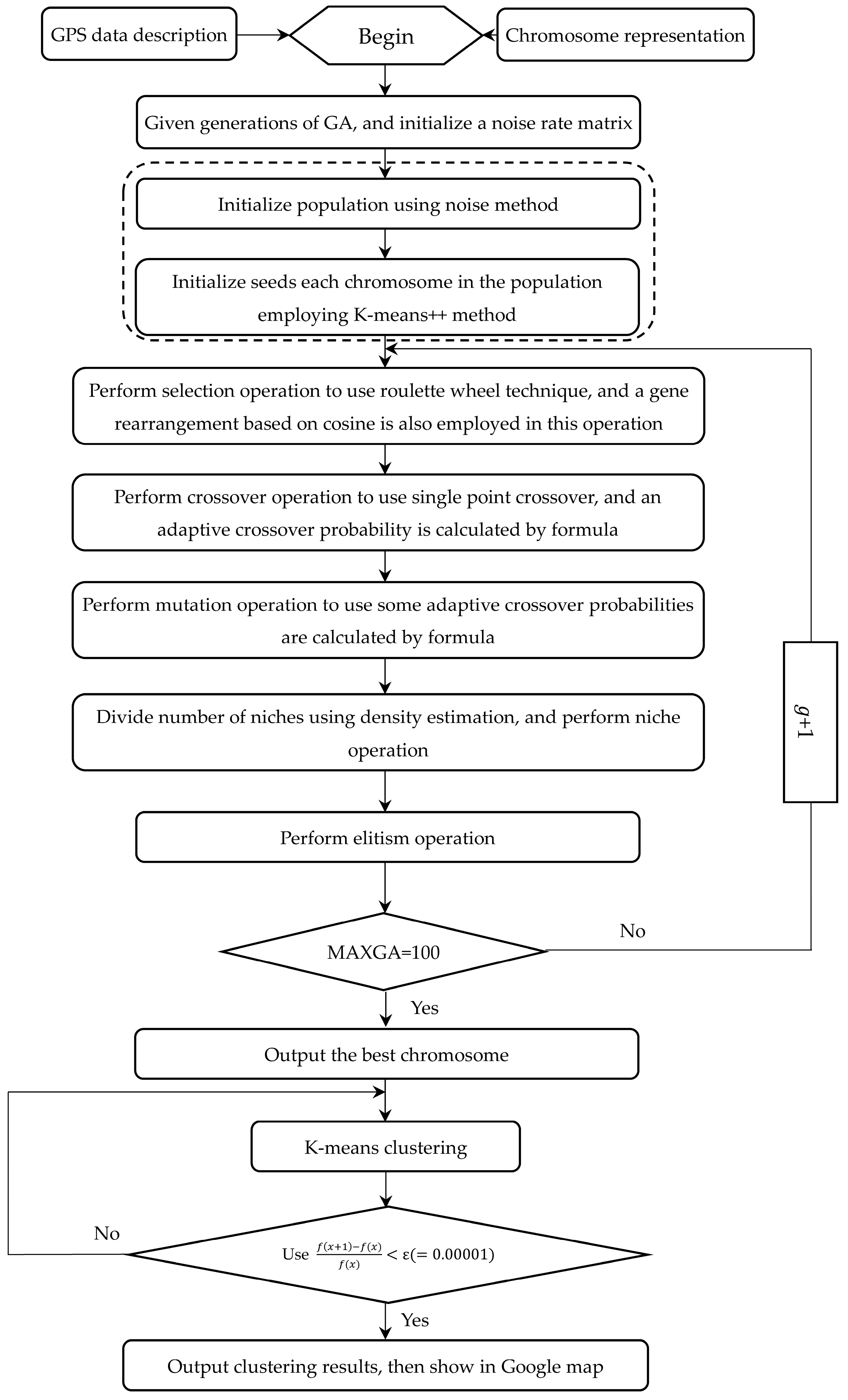
2. The NoiseClust Clustering Algorithm

NoiseClust is based on OD of the use in trajectory, and finds the best cluster centers of OD in the city. Figure 1 gives an overview of the NoiseClust algorithm including some steps as follows: (1) given a description of the taxi GPS data, our approach first used four taxi GPS data sets to explain the OD of the GPS data based trajectory (see Section 2.1); (2) real taxi GPS data sequences are used to encode chromosomes (see Section 2.2); (3) an initial population approach is proposed using noise, and K-means++ to initialize seeds (see Section 2.3); (4) DBI (Davis–Boudin index) [32] is employed as a fitness function; (5) in the genetic operation, a gene rearrangement technique based on cosine, and adaptive probabilities of crossover and mutation, are used for genetic operation (see Section 2.5); (6) a density estimation method is presented to divide the number of niches, and a share function also is used for the genetic operation, which are considered as the niche genetic algorithm (NGA) (see Section 2.6); (7) in Section 2.7, an elitism strategy is used to select the best chromosome, which is used to replace the worst chromosome in the current iteration; (8) the best chromosome is obtained to use K-means clustering; (9) the termination condition of K-means clustering is given in Section 2.9; and (10) the complexity of the NoiseClust algorithm is analyzed in Section 2.1.

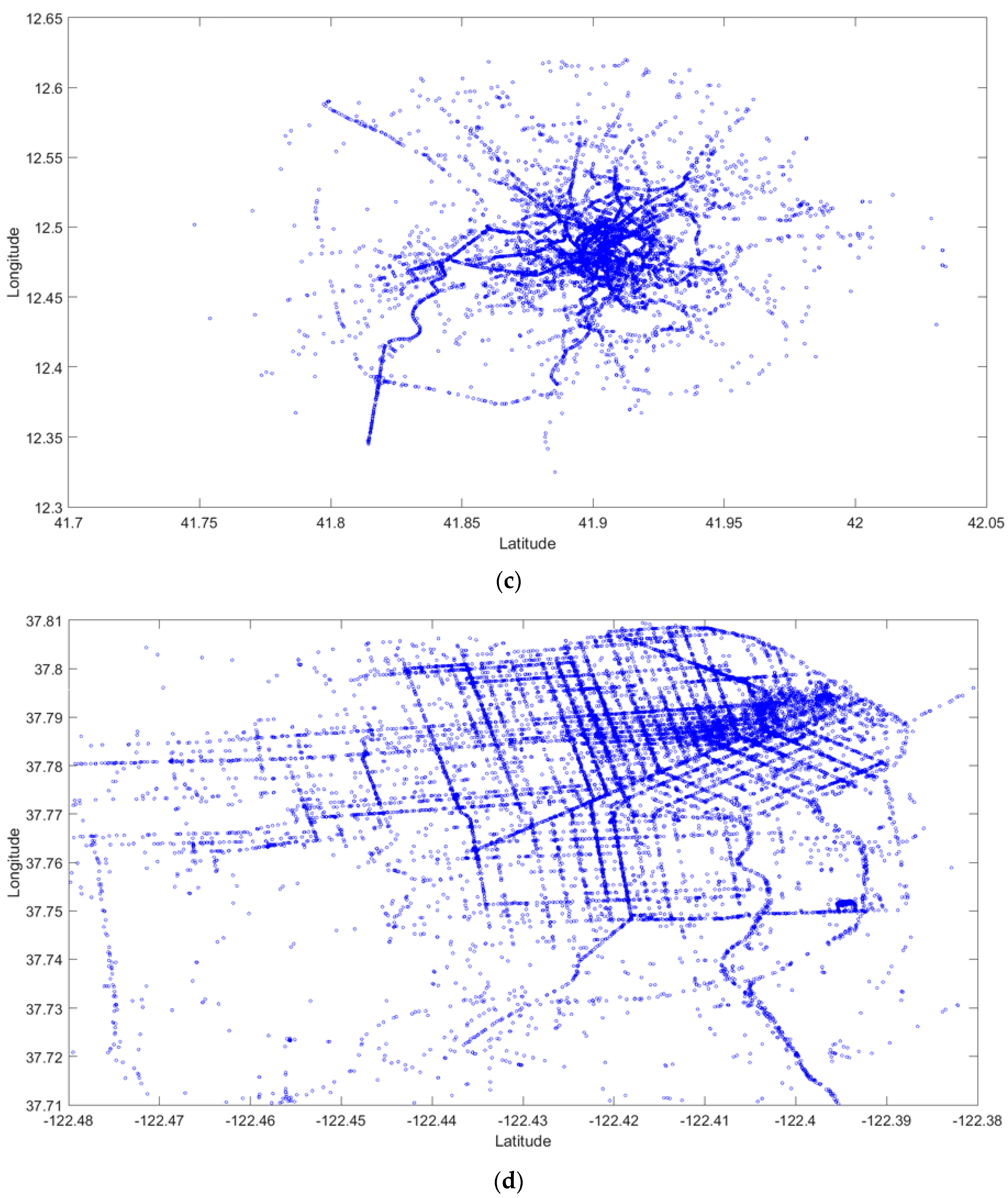
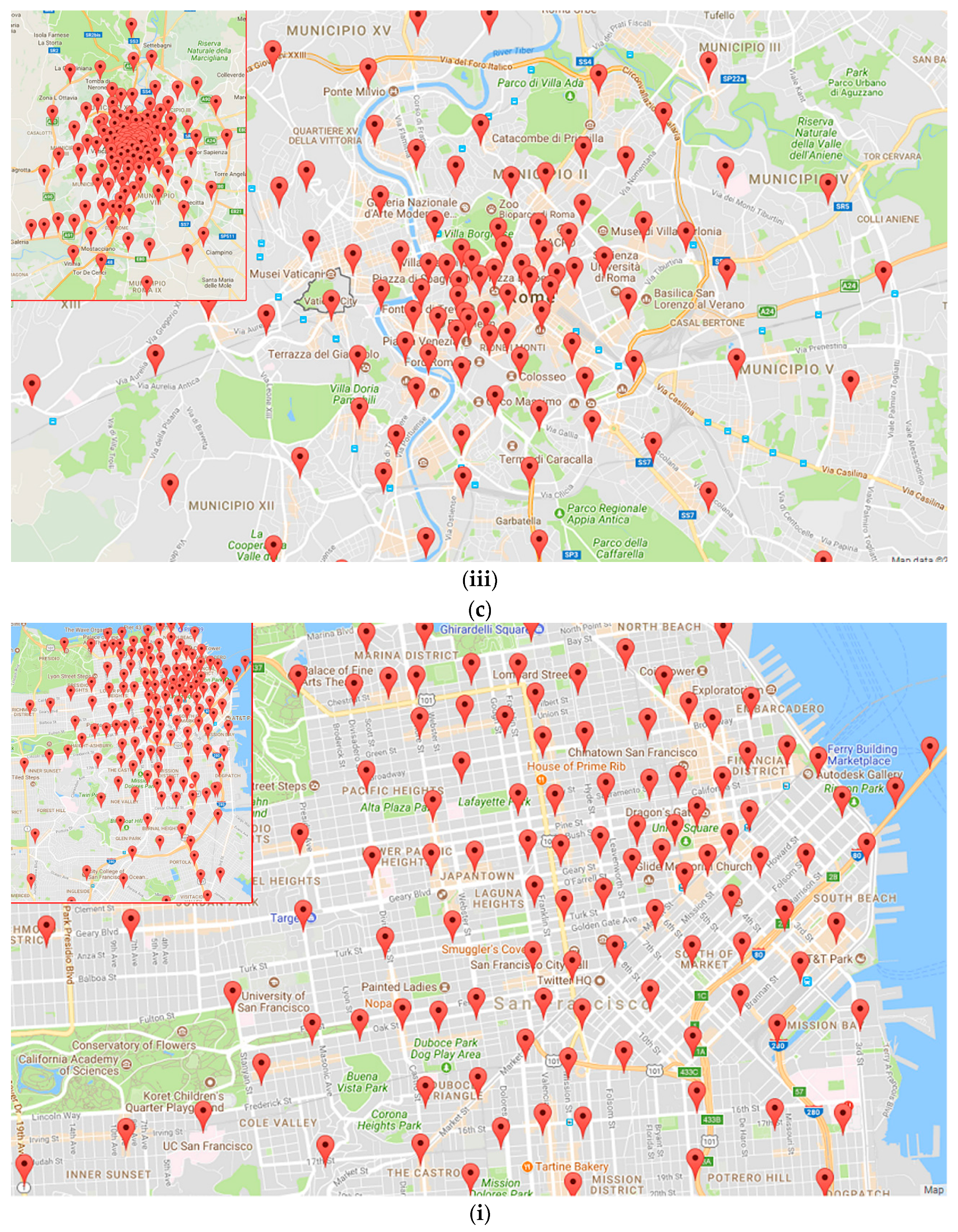
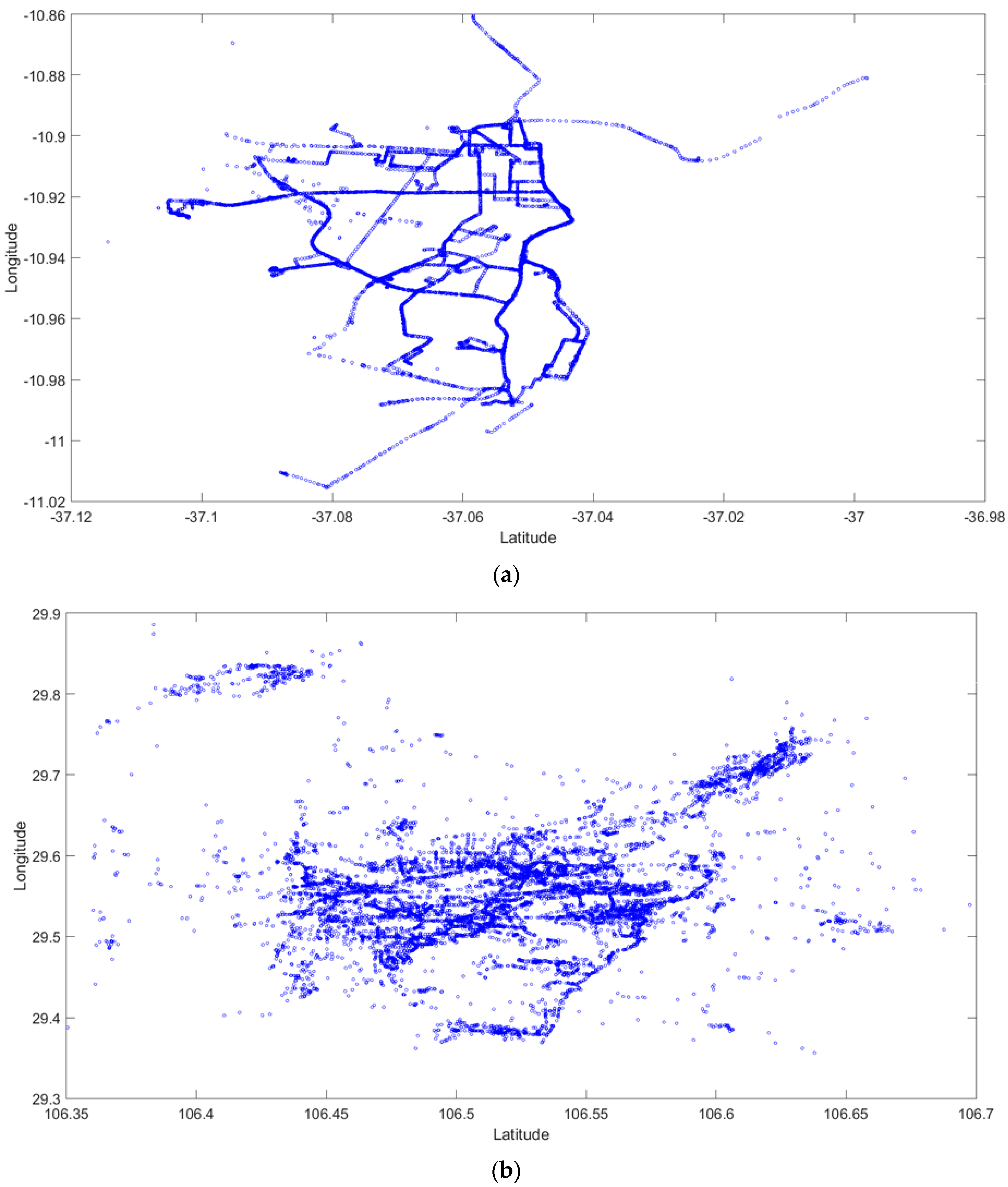
2.1. GPS Data Description

In general, a trajectory consists of many GPS location points, and GPS data based on trajectory data not only contains location information (longitude and latitude), but also collects time and status (e.g., speed, orientation and status) [33,34]. These trajectory patterns of location can be usually described by OD [2,3,4]. In this paper, the GPS data were gathered from taxi GPS points in Aracaju (Brazil), Chongqing (China), Roma (Italy), and San Francisco (USA) [35] (Figure 2a–d). However, although we can obtain the distributions of OD, it is more important to understand which area in a city can attract more people, and what the spatial distributions of these attracting locations are. Therefore, to analyze/compare the NoiseClust, GAK, and GenClust algorithms and achieve OD clustering, the taxi GPS data sets are collected and divided into OD, which are then used to encode chromosomes of genetic operation (see Section 2.2).

Figure 2 displays the distributions of taxis’ OD in a road network of the given land areas (see

Table 1. The experimental datasets of taxi GPS data.

Taxi GPS Data Set	Land Area	The Number of Taxi GPS Data Points	The Number of Clusters
			GAK	GenClust	NoiseClust
Aracaju (Brazil)	0.14 × 0.16	16,513	100	119	126
Chongqing (China)	0.60 × 0.36	19,149	100	138	138
Roma (Italy)	0.35 × 0.50	20,254	100	134	138
San Francisco (USA)	0.10 × 0.10	21,826	100	147	146

) within two minutes at each city, and the overall distributions of OD reflect the traffic change demand of citizens and population migration who use taxicabs as a transportation tool. As a result, the better cluster centers will be captured and can be used to dispatch taxis and find passengers. Furthermore, traffic information and the population migration distribution will be also obtained in order to explain each city’s situation.

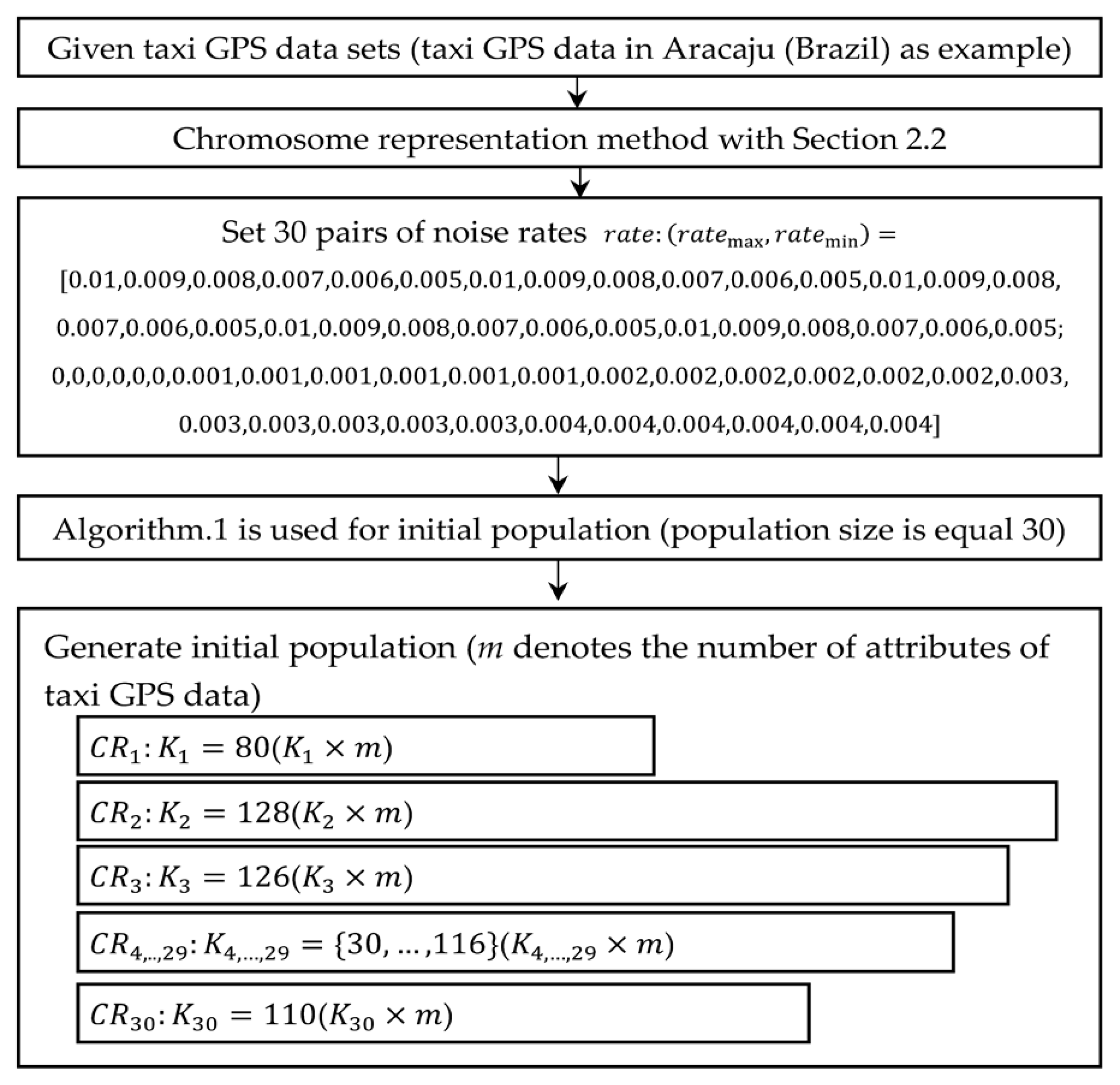
2.2. Chromosome Representation Using a Real-World Data Sequence

For any GA, each chromosome is made up of a sequence of gene coding such as binary digits, floating-numbers, integers, symbols (i.e., a, b, c, d), and chromosome representation is needed to describe each chromosome in the population. Gene coding of chromosomes determines how the optimized problem and genetic operators are structured in the algorithm that are used, and the different gene representations of the chromosomes determine the genetic performance in the population. In early GAs, 0, 1 binary digits are usually used, and it has been shown that more natural representations can obtain a more efficient and better optimal solution. However, with the increase of the length of the 0, 1 strings, more CPU computing time is needed, which causes the genetic performance to decline [20,22,36]. Therefore, OD representation is utilized to describe the chromosome in this paper; furthermore, a noise method is proposed to use the chromosomes initial selection where K-means++ is also used to select the initial seeds (see Section 2.3). Each seed of the cluster is represented by the chromosome in the same way as the NoiseClust algorithm. The number of genes of a chromosome is randomly chosen between $\left[2,\sqrt{n}\right]$ [37], where n is the number of GPS data points. Additionally, each chromosome has a different gene in size and shape, namely, when each seed no longer changed, corresponding to the cluster center being determined. Therefore, chromosome representation is described by OD as follows: a chromosome can be defined by $CR\left(G_{i1},G_{i2},\dots ,G_{iK}\right)$, or $CR\left(See{d}_{i1},See{d}_{i2},\dots ,See{d}_{iK}\right)$, namely, a gene is also regarded as a seed, and a chromosome consists of seeds in the clustering algorithms [16,23], in clustering processing, where, CR, G, K, i denotes chromosomes, genes, the number of genes of clusters ($\left[2\le K\le \sqrt{n}\right]$), and the number of GPS data points in cluster, respectively; note that a chromosome is cluster. Therefore, the chromosomes are made up of real taxi GPS data representing the seeds (cluster centers) in the initial population.

2.3. Initial Population Using Noise and K-Means++ Method

The noise method guiding the heuristic search produces to explore the solution space has led to the proposal of the recent combinatorial optimization metaheuristics technique [38], which has been applied to K-means clustering [22], as well as other application fields of the noising method such as task allocation [39], and the clique partitioning problem [40]. In addition, the noise method considers the optimal results as the outcome of a series of fluctuating data converging towards the genuine ones, and the features and the variants of the noise method are detailed, the tunings of their parameters when are applied to different combinatorial optimization problems have been summarized in [36]. Compared with other metaheuristics based on elementary transformations, the noise method is not only based on elementary transformations, but also on a descent. This noise method is randomly chosen into an interval where the range decreases during the process. For example, if we draw the noise into the interval [−rate, +rate] with a given probability distribution in the taxi GPS data sets, then the noise rate decreases during the running of the iteration process. When the objective function $f\left(1/SSE\right)$ (sum of squared errors (SSE) used to calculate noise value) [19] value for a given solution is considered, a perturbation called a noise is added to this value. Next, the noise is randomly chosen in an interval where the range decreases during the iteration process. This means that the original value of the noise rate rate, should be chosen in such a way that, at the beginning of the noise iteration process, a bad neighboring solution may be accepted. As added noises are chosen in [−rate, +rate] centered on zero, namely, the mean and the standard deviation of the rate tend towards 0 and the standard deviation during this process, a good neighboring solution may be rejected, so it induces a neighboring with $NS=b\left(b-3\right)/2$ as the elementary transformation of the noise operation [36]. This is a quick and easy way to evaluate the consequences involved by the transformation, where NS denotes the size of the neighboring, and b denotes the number of binary bits of neighborhood in the elementary transformations. The final solution is the best solution captured during the noise iteration process.

At the iteration process of noise computing, to capture the initial seeds of the clustering, the K-means++ [25] method is employed to handle the objective function value, and control the decreasing-rate. For example, if the noise rate rate decreases arithmetically, it decreases by $\left(rat{e}_{\max }-rat{e}_{\min }\right)/N$ after each trial-cluster, where the meaning of N is explained in Algorithm 1. Meanwhile, K-means++ may be an easy and quick way to evaluate the consequences involved by the elementary transformation; furthermore, it is easy to capture the number of the initial clusters and achieve population initialization. For example, for taxi GPS data sets in Aracaju (Brazil) (see Figure 2a), when the population size is equal to 30, 30 difference clusters (the number of clusters $K_i\left(i=1,\dots ,30\right)$) are initialized by 30 interval rate values of the noise method. As a result, the different size and shape of the genes are produced in 30 chromosomes, and initial seeds are also obtained. Ultimately, population initialization is also achieved, as shown in Figure 3. The structure of the algorithm is shown in Algorithm 1.

Algorithm 1. Initial population using noise and K-means++

Function: KMeanPlus (data, solution, dimension)//K-means++ [25] is employed to handle objective function value of noise, select initial seeds, and control the decreasing-rate Input: $rat{e}_{max},rat{e}_{min}$//give a group of the maximum and minimum noise rates (e.g., 30 pairs of noise rates), they are usually equal to population size.   NIND//population size (for example NIND = 30).   total_noise_ele_num//give the total number of noised elementary, it is usually equal the number of iterations which is used to noising operation.   noise_ele_num//give the number of noised elementary, it is usually equal to population size, or set number of noised elementary.   NS//it is the size of the neighborhood.   data//input taxi GPS data sets Output: initial population Procedure:   FOR 1 to NIND    draw the initial current solution s randomly (s, chrom_s(K)) ← Call KMeanPlus (data, s, m)//calculate objective function of noise, and initial seeds, chrom_s denotes seeds of chromosome using K-means ++.    best_sol ← s//it is the best solution found since the beginning    best_sol(K) ← s//obtain number of clusters each chromosome    best_chrom_sol ← chrom_s(K)//produce a chromosome to put into population    $decrease\leftarrow (rat{e}_{max}-rat{e}_{min})/\left[\left(total\_noise\_ele\_num-noise\_ele\_num\right)-1\right]$//denote the value by which rate decrease.    $restart\leftarrow \sqrt{total\_noise\_ele\_num·NS}$//gives the frequency of the restart of the current solution    $rate\leftarrow rat{e}_{max}$//give the current value of the noise rate    $initial\_iteration\leftarrow 0$//count the number of noise trial which have been applied.   WHILE $initial\_iteration<total\_noise\_ele\_num$   $initial\_iteration\leftarrow initial\_iteration$ + 1    IF $rate!=0$     $r\_rate$←rate    END    solution s translate into binary bits and produce next solution s’//let s’ be the next neighbor of s    solution s’ translate into decimal value K and determine K range between 2 and $\sqrt{n}$//produce the number of clusters    let noise be a random real number uniformly drawn into $\left[-rate,rate\right]$    search s’//search one of its neighbors    IF s’ = ∅     $\left(s^{\prime },chrom\_s\left(K\right)\right)\to$ Call KMeanPlus (data, s’, m)     best_sol ← s’    ELSE     perform solution $\left(s,chrom\_s\left(K\right)\right)$ for taxi GPS data sets to start producing chromosome    END    IF $f\left(s^{\prime }\right)-f\left(s\right)+noise<0$     s ← s’     $chrom\_s\left(K\right)$ is controlled to produce chromosome    END    IF $\mathrm{mod}\left(initia{l}_{iteration},4*NS\right)==0$//mod is modulo     $rate=0$ //apply noise rate (=0) descent from s result in a good neighboring solution may be rejected    END    IF $f\left(s\right)<f\left(best\_sol\right)$     $best\_sol$ ← s     s ← best_sol(K)     best_chrom_sol ← chrom_s(K)    END    IF $\mathrm{mod}\left(initial\_iteration,restart\right)==0$     s ← $best\_sol$     best_sol(K) ← s    END    IF $\mathrm{mod}\left(initial\_iteration,noise\_ele\_num\right)==0$     IF $rate!=0$      rate = rate − decrease     ELSE      rate = r_rate − decrease     END    END   END    produce a chromosome and record length of its (the number of clusters)   END    achieve population (30 chromosomes) initialization

2.4. Fitness Function

The fitness function is used to define a fitness value to each candidate solution. The common clustering criterion or quality indicators mainly include the SSE, DBI (Davis–Boudin index), Dunn’s index, Xie-Beni index, PBM (PBM-index), and COSEC (compactness and separation measure of cluster) [16,31], which can be used as fitness functions for GA. In this paper, the DBI is used as the clustering measure. The idea of the Davis-Boudin index [32] is to minimize the intra-cluster distance, while maximizing the distances among the different clusters, and is defined as:

$$DBI=\frac{1}{K}{\displaystyle \sum }_{i=1}^K\underset{i\ne j}{\max }\left(\frac{{{\displaystyle \sum }}_{G_i\in C{R}_i}{d}^2\left(CR,see{d}_i\right)+{{\displaystyle \sum }}_{G_j\in C{R}_j}{d}^2\left(CR,see{d}_j\right)}{d^2\left(see{d}_i,see{d}_j\right)}\right)$$

where, due to the DBI, small values of the DBI correspond to compact and well-separated clusters. This index does not present a monotonic behavior with K, so the DBI also allows the optimal number of clusters for the given taxi GPS data set to be validated.

Then, the fitness function of the chromosome is defined as the inverse of DBI, i.e.,

$$f=\frac{1}{DBI}$$

This fitness function will be maximized during the evolutionary process for the NGA for each iteration and leads to the minimization of the DBI.

2.5. Genetic Operations

This section mainly discusses the method used to handle genetic operation, and adaptive probabilities of crossover and mutation are also employed to prevent the convergence to a local optimum without defining the genetic parameter.

2.5.1. Selection Operation

Chromosomes (e.g., NIND = 30) are sorted by descending order of their fitness values, then the number of the best chromosomes are chosen from the initial population of the NIND chromosomes using the fitness function, which generate a selection population $PO{P}_s$. The maximum fitness value is selected from chromosomes according to the descending order of their fitness values. A copy of the best chromosome is stored in the memory.

2.5.2. Crossover Operation

To handle the different size and shape of the genes, an improved gene rearrangement operation is first presented, then the crossover operation is performed.

Several existing gene rearrangement techniques [20,41] considered the lengths of both chromosomes as equal and were therefore unable to rearrange the genes if the lengths of the chromosomes were not equal [16]. This is a novel gene rearrangement technique, which can handle chromosomes of unequal lengths, but it only focuses on gene rearrangement operations without considering between the structure chromosomes, resulting in difficulty in determining the reference chromosome and target chromosome. Therefore, we first obtain the best chromosome in descending order according to its fitness values, and a pair of chromosomes are chosen using an existing roulette wheel technique (RWT) [22,28] where the chromosomes $C{R}_i,C{R}_j$ are picked with the probability $p\left(C{R}_i,C{R}_j\right)=f\left(C{R}_i,C{R}_j\right)/{\displaystyle \sum }_{i=1,j=i+1}^{NIND}f\left(C{R}_i,C{R}_j\right)$. Here, $f\left(C{R}_i,C{R}_j\right)$ is the fitness of the pair of chromosomes $C{R}_i, C{R}_j$, and NIND is the size of the current population. Next, we use the cosine theorem to calculate the similarity of values between the chromosomes producing triangle planes. When the cosine similarity between the chromosomes have unequal length, 0 as genes are added into chromosomes to guarantee the same genes in each chromosome. To obtain a useful reference chromosome and target chromosome, these similarity values are translated into angles and the maximum angle of the triangle corresponded to the “triangle side” of the reference chromosome, and the minimum angle of the triangle corresponded to the “triangle side” of the target chromosome. Finally, the gene rearrangement method in [16] is employed to perform the gene rearrangement operation, which rearranges the genes of the inferior chromosome (called the target chromosome) with respect to the gene arrangement of the superior chromosome (called the reference chromosome). The similarity based on the cosine theorem is computed as

$$Sim\left(C{R}_i,C{R}_j\right)=\frac{{{\displaystyle \sum }}_{i,j=1}^{NIND}\left(C{R}_i-C{R}_b\right)\left(C{R}_j-C{R}_b\right)}{\sqrt{{{\displaystyle \sum }}_{i=1}^{NIND}{\left(C{R}_i-C{R}_b\right)}^2}\sqrt{{{\displaystyle \sum }}_{j=1}^{NIND}{\left(C{R}_j-C{R}_b\right)}^2}}$$

where $C{R}_{ik} ,C{R}_{jk}$ are made of a number of genes in each chromosome, and the Euclidean distance between the taxi GPS data points are shorter and more similar; $C{R}_i,C{R}_j$ are two chromosomes vectors; and $C{R}_b$ stands for the best chromosome with the fitness in the current iteration.

The main goal of the crossover operation is to create diversity, potentially producing new chromosomes using gene rearrangement and crossover probability. According to their fitness values, chromosomes are sorted by descending order. All chromosomes (selection population) participate in the crossover operation in terms of gene rearrangement. Then, it combines the features of two parent chromosomes to produce two offspring using a single point crossover operation $SPC\left(C{R}_i,C{R}_j,\alpha \right)$, which is calculated according to [16,20], where each chromosome is divided into two parts at a random point between two genes. The crossover operation is an information exchange between different potential solutions, and the crossover probability $P_c$ is calculated. From the crossover of a pair of chromosomes, we obtain a pair of offspring chromosomes, which are added to the population of the next generation, and every time a chromosome is chosen, it is removed from the population of the current generation [18].

The point crossover operation is calculated as:

$$SPC\left(C{R}_i,C{R}_j,\alpha \right)=\{\begin{array}{c}C{R}_i^{\prime }=\alpha C{R}_j+\left(1-\alpha \right)C{R}_i\\ C{R}_j^{\prime }=\alpha C{R}_i+\left(1-\alpha \right)C{R}_j\end{array}$$

where $\alpha$ is a crossover parameter and $\alpha \in \left(0,1\right)$.

The crossover probability is calculated as:

$$P_c=\{\begin{array}{c}\frac{f_{\max }-f^{\prime }}{f_{\max }-f_{\mathrm{avg}}} \mathrm{if} f^{\prime }>f_{\mathrm{avg}} \\ 1 \mathrm{if} f^{\prime }\le f_{\mathrm{avg}}\end{array}$$

where $f_{\max }$ denotes the maximum fitness value of the current population; $f_{\mathrm{avg}}$ denotes the average fitness value of the population; and $f^{\prime }$ denotes the larger of the fitness of the chromosomes to be crossed. The value of $P_c$ increases when the chromosome is quite poor. In contrast, when the chromosome is a good solution, $P_c$ is low to reduce the likelihood of disrupting a good solution by crossover.

The whole process of the gene pair selection and crossover operation continues while there are genes in the population, and we obtain chromosomes to generate the crossover population $PO{P}_c$, which are used for the next generation.

2.5.3. Mutation Operation

The basic idea of the mutation operation is to randomly alter one or more genes of a selected chromosome to explore different solutions. The mutation operator includes small modifications to each chromosome in the population, with low fitness having a high probability of randomly changing using the mutation probability calculation formula, to explore new regions of the search space and to also escape from the local optima when the algorithm is near convergence [21], with the random change having a probability equal to the mutation rate. The intuition behind the mutation operation is to introduce extra variability into the population [20], and the mutation probability of each chromosome in the crossover population is calculated. The mutation probability of the ith chromosome is given as follows:

$$P_m=\{\begin{array}{c}{\xi }_1\times \frac{f_{\max }-f_i}{f_{\max }-f_{\mathrm{avg}}} \mathrm{if} f>f_{\mathrm{avg}}\\ {\xi }_2 \mathrm{if} f\le f_{\mathrm{avg}}\end{array}$$

where ${\xi }_1, {\xi }_2$ are equal to 0.5; $f_{\max },f_{\mathrm{avg}}$ are the same as defined above; and $f_i$ is the fitness of the ith chromosome under mutation. When $P_m>P_c$, the high fitness solutions rapidly aid in the convergence of the NGA, but the low fitness values cannot prevent the GA from getting stuck at a local optimum. To prevent the GA from getting stuck at a local optimum, the solutions with fitness values are used to reduce the mutation probability and search the search space for the region containing the global optimum.

The mutation process utilized in this paper is the same as that used in [21,42], which is calculated as follows:

$$R=\{\begin{array}{c}\frac{f-f_{\min }}{f_{\max }-f_{\min }} \mathrm{if} f_{\max }>f\\ 1 \mathrm{if} f_{\max }>f_{\min }\end{array}$$

where $f_{\max }$ and $f_{\min }$ are the maximum and minimum fitness values in the current population. For a chromosome with fitness value $f$, a number $\delta$ in the range $\delta \in \left[-R,R\right]$ is generated with a uniform distribution.

If the maximum and minimum values of the GPS data set along the ith dimension are $f_{\max }^i$ and $f_{\min }^i$, respectively, then after mutation, the ith gene of the chromosome is defined as follows:

$$f^{i^{\prime }}=\{\begin{array}{c}{f}^i+\delta \times \left(f_{\max }^i-f^i\right)\\ f^i+\delta \times \left(f^i-f_{\min }^i\right)\end{array}$$

After the mutation operator, if they have the same genes in each chromosome, the twin removal operation in [16] is employed to remove twin genes from each chromosome producing a mutation population $PO{P}_m$, and we again update the chromosome with the best fitness at this stage (mutation operator).

2.6. Sharing-Based Niche Partitioning Using Density

This section mainly aims to maintain a population diversity and prevent premature convergence using the niche technique. We divide the population into a number of niches using a density-based method, then a sharing-based niching method is presented to adjust the sharing fitness values.

2.6.1. Niches Partitioning Based on Density

The density-based method has been widely used in clustering works from large scale data for its simple calculation structure and low computing cost [6,33,43]. In this paper, the density-based method is used to divide the number of niches, directly divides all the point densities reachable from different points into the niches, and is meaningful in finding an appropriate method to estimate the density using a given radius r. In other words, a given density radius r is placed in taxi GPS data sets to draw some circles (density), and the number of taxi GPS points (density) are counted in each circle, then these densities are sorted in term of the number of taxi GPS points in each circle. Finally, the maximum density as a niche is obtained; and the above operations are repeated until all the taxi GPS points are selected, as shown in Algorithm 2. As a result, it indicates that the number of niches has been obtained.

Algorithm 2. Niches partitioning based on density

Input: GPS taxi data (data), a given density radius r Output: result of the niche partitioning, including number of niches, and number of GPS points each niche Procedure: WHILE data = = ∅   Num_circles ← radius r is placed in taxi GPS data sets//Num_circle denotes the number of densities   Num_points ← counts the number of taxi GPS points each density and record in Num_points   Num_niches ← sort Num_points in the ascending order according to the number of taxi GPS points, and obtain a maximum density to separate storage.   The remaining taxi GPS points continue operation until data = = ∅ END WHILE

2.6.2. Sharing-Based Niche Method

NGA has been proved that when the number of chromosomes within the population is large enough and the niche radius is properly set, a sharing function provides as many niches in the population as the number of peaks in the fitness landscape [44,45]. However, there are several problems such as stability and maintainability [45]. To improve this performance and overcome the sharing level of niches, a modification of the niching method is introduced and integrated into our approach, in order to preserve the population diversity during the simultaneous search for a global optimum. Our approach can maintain the population diversity with respect to the new population with mutation operator $PO{P}_m$ adjusts in the solutions. An initial niching population is generated by the mutation operation (for instance, a new population can be defined as: $PO{P}_{\mathrm{new}}= PO{P}_m+ \frac{2}{3}PO{P}_s$). In this paper, the fitness sharing modifies the search range by reducing the fitness of a chromosome in densely-populated regions. It works by derating the fitness of each chromosome by an amount related to the number of similar chromosomes in the new population. In particular, the shared fitness $f_{\mathrm{share}}\left(i\right)$ of each chromosome i in generation g of the number of the partitioning niches nich is defined as follows, and we again obtained the chromosome $C{R}_{best,g}$ with the best fitness each iteration:

$$f_{\mathrm{share},nich}\left(i\right)=\frac{f_g\left(i\right)}{s_{g,nich}\left(i\right)}$$

where $f_g\left(i\right)$ is the current fitness of the chromosome; and $s_{g,nich}\left(i\right)$ is the sum of niche sharing dependent on the number of the partitioning niches and each iteration of the chromosomes within the population. The sum of niche sharing degree each iteration is calculated as:

$$s_{g,nich}\left(i\right)={\displaystyle \sum }_{i=1}^{nich}share\left(simi\left(C{R}_{best,g},C{R}_i\right)\right)$$

where $simi\left(C{R}_{best,g},C{R}_i\right)$ denotes the similarity between the best fitness values of the chromosome and the current chromosome i using Pearson correlation-based similarity measure [28] in the new population; and $simi$ is the sharing function which measures the sharing degree between the two chromosomes; additionally, the number of niches nich is obtained in Section 2.6.1. The most common method is defined as:

$$Share\left(simi\left(C{R}_{best,g},C{R}_i\right)\right)=\{\begin{array}{c}1-{\left(\frac{simi\left(C{R}_{best,g},C{R}_i\right)}{{\sigma }_{\mathrm{share}}}\right)}^2 \mathrm{if} simi\left(C{R}_{best,g},C{R}_i\right)\le {\sigma }_{\mathrm{share}}\\ 0 \mathrm{otherwise} \end{array}$$

where ${\sigma }_{\mathrm{share}}$ is the niche radius, which is calculated as per [46], and $\left|C{R}_{\mathrm{best}}\right|$ is the number of genes of the best chromosome according to its fitness value order; $\left|PO{P}_{\mathrm{new}}\right|$ is the number of chromosomes in the new population.

$${\sigma }_{\mathrm{share}}=\frac{\sqrt{\left|PO{P}_{\mathrm{new}}\right|}}{2\times \sqrt[\left|PO{P}_{\mathrm{new}}\right|]{\left|C{R}_{\mathrm{best}}\right|}}$$

A gene expression data consisting of n genes (taxi GPS data points) and d chromosomes are usually expressed as a real valued $n \times d$ matrix $E=\left[G_{ij}\right],i=1,\dots ,n, j=1,\dots ,d$. Here, each element $G_{ij}$ denotes the expression level of the ith gene at the jth chromosome. When the Pearson similarity between the chromosomes are unequal in length, 0 as genes are added into the chromosomes to guarantee the same genes in each chromosome. Therefore, given two chromosome vectors $C{R}_i$ and $C{R}_j$, the Pearson correlation coefficient $simi\left(C{R}_i,C{R}_j\right)$ between them is calculated as

$$simi\left(C{R}_i,C{R}_j\right)=\frac{{{\displaystyle \sum }}_{l=1}^d\left(G_{il}-{\mu }_{G_i}\right)\left(G_{jl}-{\mu }_{G_j}\right)}{\sqrt{{{\displaystyle \sum }}_{l=1}^d{\left(G_{il}-{\mu }_{G_i}\right)}^2}\sqrt{{{\displaystyle \sum }}_{l=1}^d{\left(G_{jl}-{\mu }_{G_j}\right)}^2}}$$

where ${\mu }_{G_i}, {\mu }_{G_j}$ represent the arithmetic means of the components of the chromosomes vectors $C{R}_i$ and $C{R}_j$, respectively.

When our approach maintains diversity and reached the global optimum, the number of niches reduced to one. After the niche operation, a new population is generated by using the elitism operator.

2.7. Elitism Operation

This keeps track of the best chromosome throughout the iterations and also keeps improving the quality of the population in each generation. Corresponding to the above results, a new elitism population is also generated, and the best chromosome is obtained by the descending order of their fitness values, which is used for the K-means clustering operation.

2.8. K-Means Clustering Using the Best Chromosome

K-means has become the most popular and compared clustering algorithm as the basic K-means requires as input a parameter of the number of clusters, which has a major dependency on the initialization of the seeds, and gets stuck in local optima. In this paper, we use the genes of the best elitism chromosome as the initial seeds, and when SSE is used as the seed updating method it achieves K-means clustering, as shown in Algorithm 3. With high-quality initial seeds, K-means is also expected to generate a high-quality clustering solution. Meanwhile, the clustering solutions based on NoiseClust are outputted on the Google map (See Section 3.2), which display the clustering results of OD.

Algorithm 3. K-means clustering using the best chromosome

Input: taxi GPS data set, the best chromosome Output: K-means clustering result Procedure:  Obtain the number of genes (K) of the best chromosome as the number of clusters;  Initialize the K seeds using genes of the best chromosome;  WHILE $\epsilon =0.00001$//when meet $\epsilon$, its number of iterations is record to x   FOR 1 to K    FOR 1 to m//repeat the number of attributes     FOR 1 to n//repeat the number of taxi GPS data points      Assign each taxi GPS data point to the closest seed;      Update the seeds from the taxi GPS data points assigned to each cluster using SSE      //SSE model is described in Section 3.1;     END FOR   END FOR    Remove empty clusters;    Remove clusters of the lesser taxi GPS points (<3) and add into the closest clusters;   END FOR  END WHILE     Output clustering results of taxi GPS data set and display in map.

2.9. Termination Condition

Our approach defines a termination condition value ε (e.g., ε = 0.00001) to try to capture the optimum clustering results in a close neighborhood of a cluster. The K-means clustering search, which is based on the ratio value between the difference of fitness value (between the current iteration and next iteration) and the current fitness value is calculated as

$$\frac{f\left(x+1\right)-f\left(x\right)}{f\left(x\right)}<\epsilon$$

where $f\left(x\right)$ denotes the fitness value of the current iteration; $f\left(x+1\right)$ represents the fitness value of the next iteration; and $x$ denotes the number of iterations for the K-means clustering operation. The implemented search works over the fitness values of the chromosomes, and this operation determines the better cluster results obtained when the termination condition is satisfied, and the GPS points are assigned to close neighborhood clusters in the solution.

2.10. Complexity Analysis of NoiseClust

In fact, the analysis used in many K-means algorithm clustering problems suffer from the number of clusters, the initial seeds, and local optimum, which can be avoided in the NoiseClust clustering algorithm. According to [16,47], considering the total number of GPS data points is n, the population size is NIND (N), the number of iterations is MAXGEN ($g$), the number of attributes is m, the number of iterations for K-means clustering is x, and the maximum number of genes in a chromosome is K. The complexity of NoiseClust is made of six parts as follows:

Initialization: This is made of noise and K-means++. According to Algorithm 1, the time complexity of the population initialization is $O\left(nmN\right)$.

Fitness function: The fitness functions of each chromosome are calculated using DBI, its complexity consisted of computing all pairs of seeds, the distances between each point and its closest seed operation, and the descending order operation. The time complexity of the fitness function is $O\left(gNn{m}^2\right)$.

Genetic operation: This is made of the selection, crossover, and mutation operation; therefore, the time complexity of genetic operation is $O\left(gN{K}^{2}m\right)$.

Niche operation: This is made of the density estimation and sharing-based computing; therefore, the time complexity of niche operation is $O\left(gN{n}^{2}m\right)$.

Elitism operation: After the niche operation, the complexity to identify the best and worst chromosomes of a generation is $O\left(g{N}^{2}m\right)$. Therefore, the total time complexity of the elitism operation is $O\left(g{N}^{2}m\right)$.

K-means operation: The time complexity of K-means clustering is $O\left(nmKx\right)$.

Therefore, the time complexity of NoiseClust is $O\left(nmN+gNn{m}^2+gN{K}^{2}m+gN{n}^{2}m+g{N}^{2}m+nmKx\right)$. The time complexity of NoiseClust is lower than GenClust [16] due to the initial population and the twin removal of GenClust needed higher complexity, the test result of time complexity is described in Section 3.2.

3. Experimental Results and Discussion

In this section, for the purpose of testing the performance of the NoiseClust algorithm, experiments are conducted on real-world taxi GPS data sets [35] (shown in Table 1), and the results show that NoiseClust has a higher performance and effectiveness than GenClust [16] and GAK [42]. Computer simulations are conducted in Matlab (v.2016a) (MathWorks, Natick, MA, USA) on an Intel (R) Xeon (R) CPU E5-2658, running at 2 @ 2.10 GHz with 32 GB of RAM in Windows Server 2008. The termination condition of clustering algorithms is $\epsilon =0.00001$. In order to use the same comparison standard described in [48], all fitness values $f$ of the NGA (and GenClust, GAK) are normalized using the following formula:

$$f_{n\mathrm{orm}}=\frac{f-f_{\min }}{f_{\max }-f_{\min }}$$

where $f_{n\mathrm{orm}}$ is the normalized value; and $f_{\max }$ and $f_{\min }$ are the maximum and minimum values of the $f$ values.

If all f values of NGA (and GenClust, GAK) are normalized by $f_{n\mathrm{orm}}$, the maximum and minimum fitness values each iteration can be 1 and 0, respectively. The aim is to compare three GA-based clustering algorithms (NoiseClust, GenClust, and GAK) using the same standard (see Figure 3a–d).

3.1. Clustering Evaluation Criteria

Validation or evaluation of the resulting clustering allow us to analyze the result in terms of objective measures [49]. Depending on the information available, the clustering results can be evaluated in terms of the Silhouette coefficient (SC) [21,50], PBM [31], and SSE [20].

This type of evaluation tries to determine the quality of an obtained partition of the data without any available external information. Therefore, three of the most useful evaluation criteria are employed as follows.

SC is a measure that has been used quite often in clustering problems since it allows the evaluation of the quality of a particular solution as well as the quality of each cluster that conforms to that solution [21,28,50]. In other words, it allows for the evaluation of a given assignment for a particular observation $G_{iK}$. SC is then defined for the jth observation $G_{jK}$:

$$SC=\frac{1}{K}{\displaystyle \sum }_{j=1}^K{\displaystyle \sum }_{x_j}\frac{a_j-b_j}{\max \left(a_j,b_j\right)}$$

where $a_j$ denotes the average distance between an observation point $G_{jK}$ and the other point vectors of the cluster to which the point is assigned; and $b_j$ denotes the minimum of the average distance obtained for all clusters different than the one assigned to $G_{jK}$. Note that the value of the SC index varies from −1 to 1, and a higher value indicates a better clustering result.

PBM [31] is used to measure the clustering performance as it can provide a measure of goodness of clustering on different partitions of a given data set, and can describe a cluster validity index of a cluster solution. Then, the fitness function maximizes the value of this PBM index:

$$PBM={\left(\frac{1}{K}\times \frac{d^2\left(G_1,see{d}_1\right)}{{{\displaystyle \sum }}_{k=1}^K{{\displaystyle \sum }}_{i=1}^n{d}^2\left(G_{iK},see{d}_{ik}\right)}\times {\max }_{i,j=1}^K\left\{d^2\left(see{d}_i,see{d}_j\right)\right\}\right)}^p$$

where n denotes the total number of GPS data points in the data set. The power p is used to control the contrast between the different cluster configurations. Here, let p = 2. A large value of the PBM index implies a better solution.

SSE is the most straightforward and popular evaluation of distance in unsupervised clustering measures. It only needs to consider the cohesion of clusters to evaluate the quality of the given partition data [21], and is defined as:

$$SSE={\displaystyle \sum }_{k=1}^K{\displaystyle \sum }_{G_i\in C{R}_i}{d}^2\left(CR,see{d}_{ik}\right)$$

where K denotes the number of clusters; and $d^2\left(CR,see{d}_i\right)$ is the distance from the observed chromosome (a chromosome is defined for a vector) CR to the seeds of the cluster k, represented by the $see{d}_{ik}$.

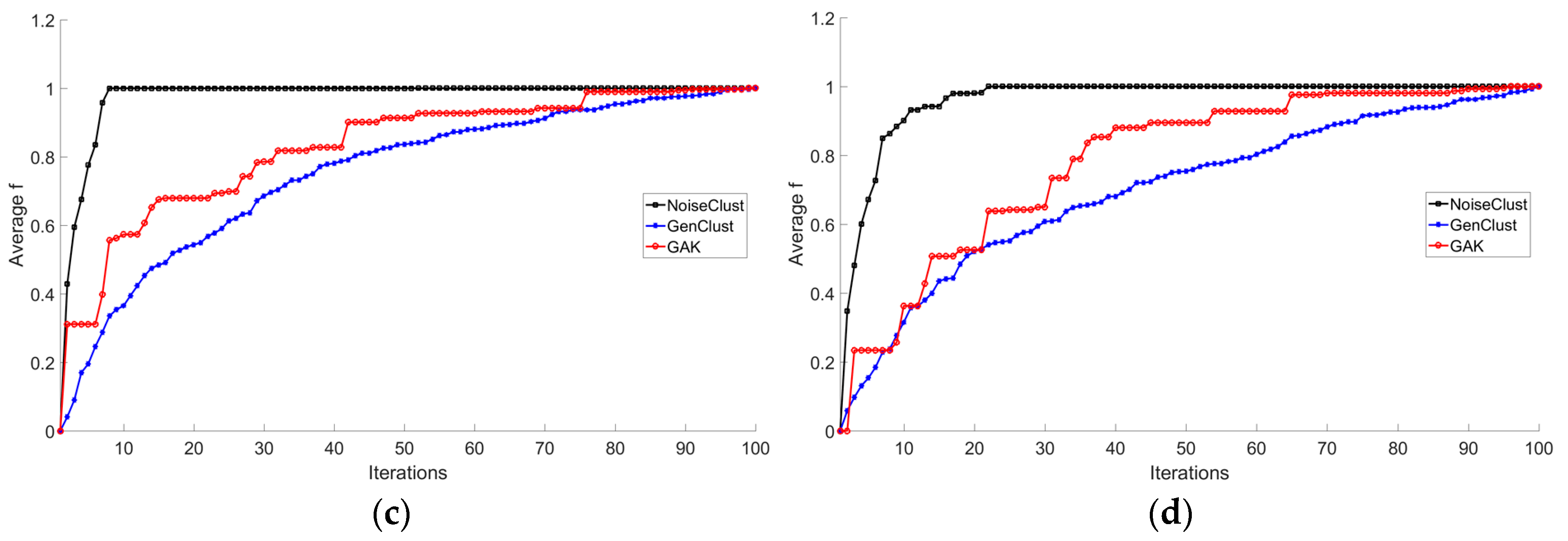
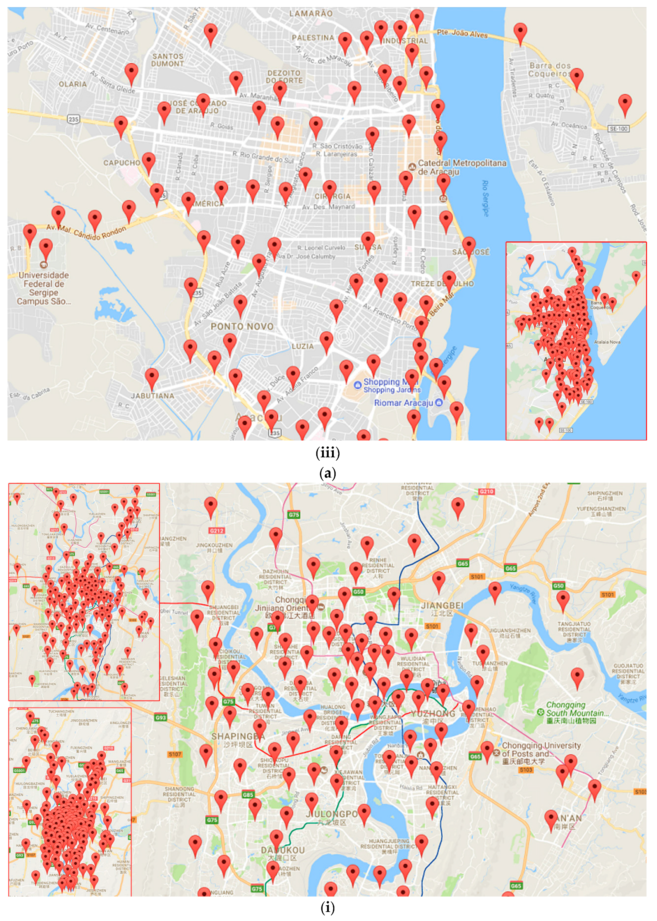
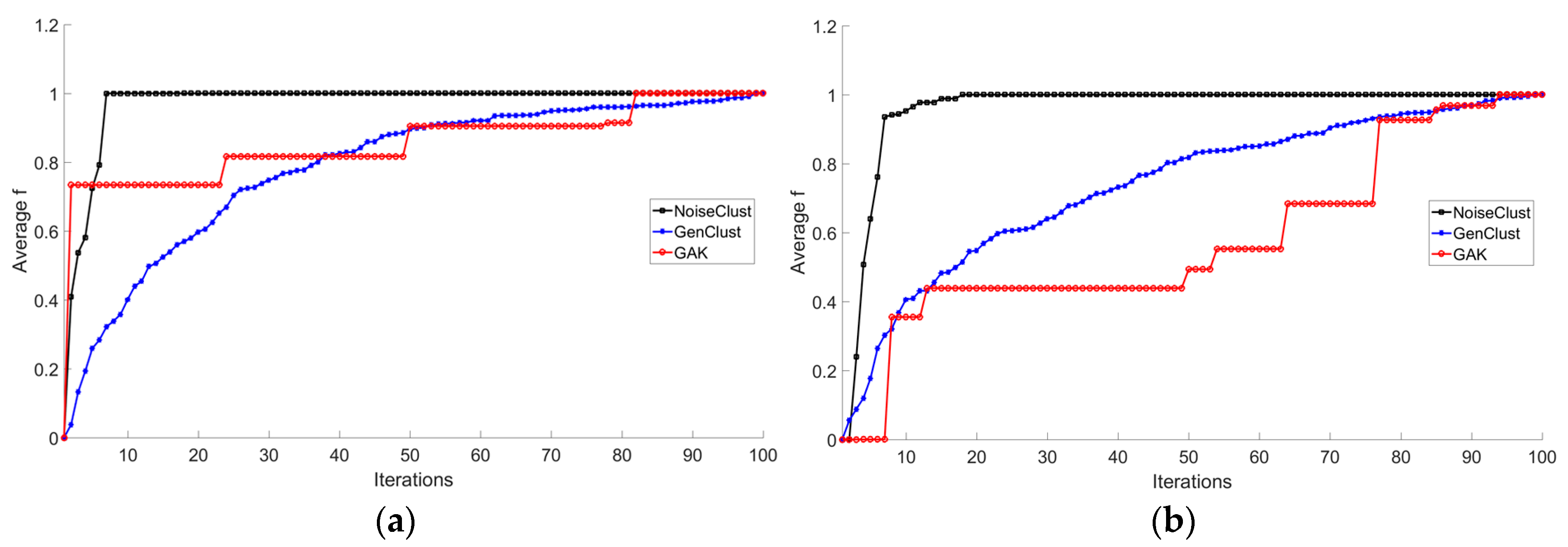
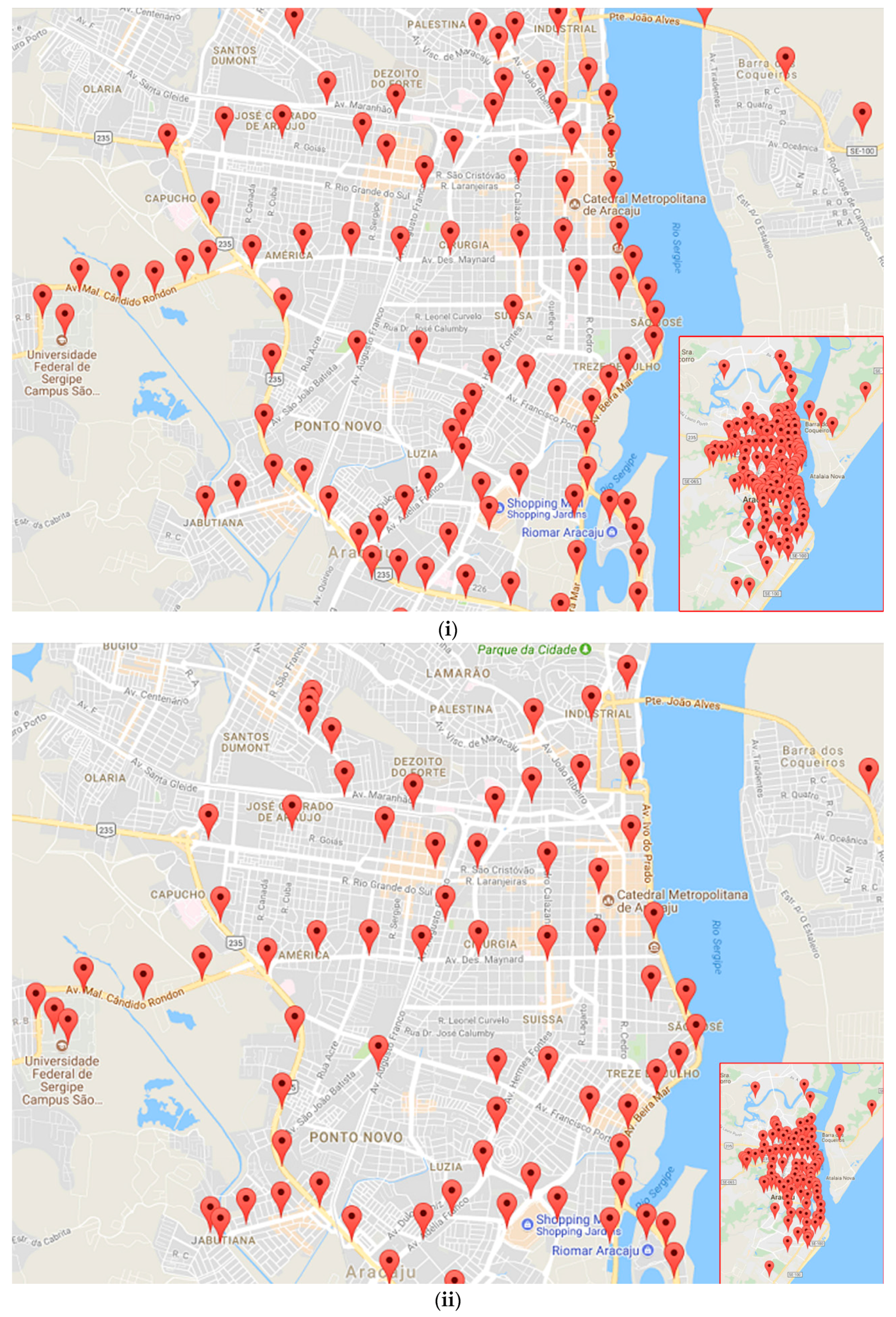
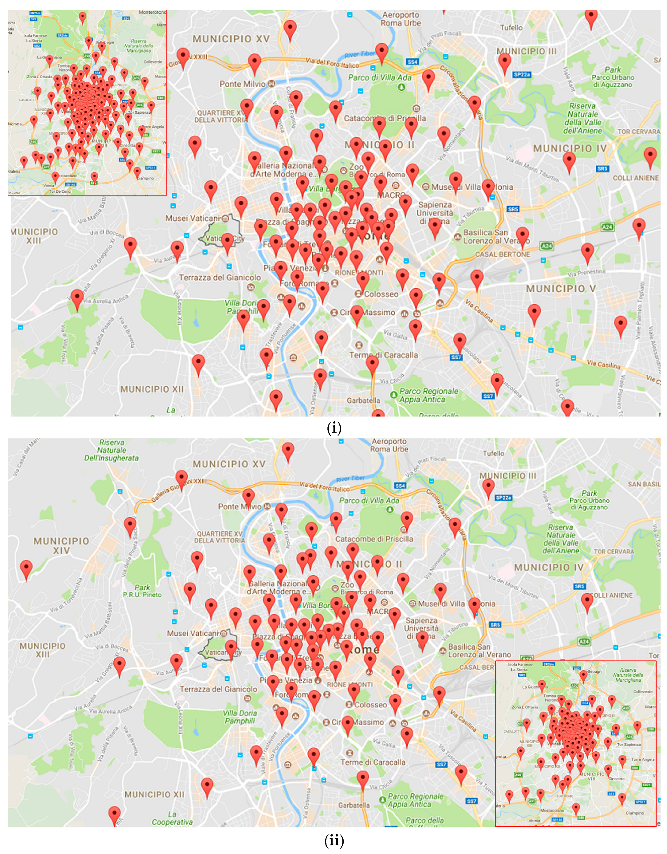
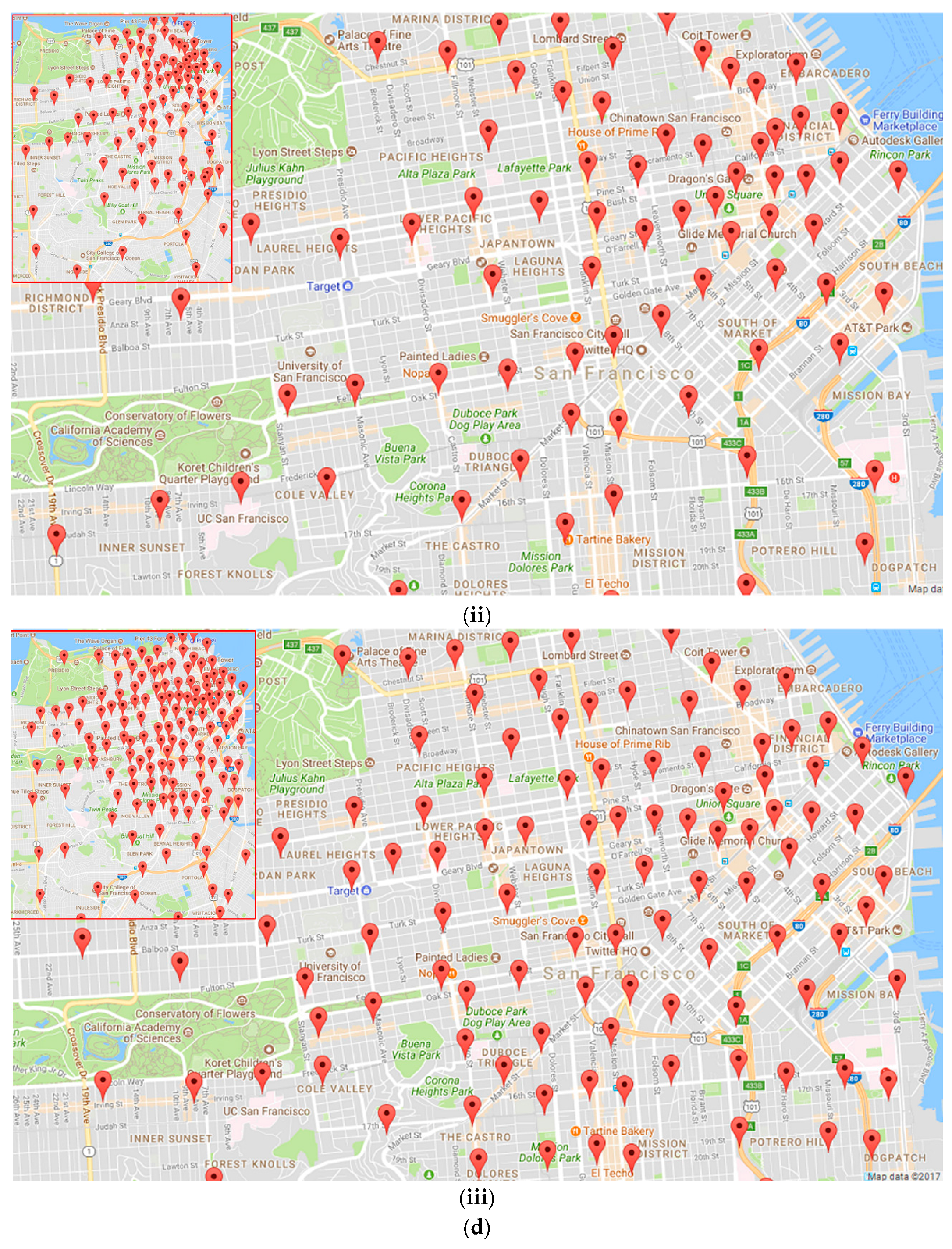
3.2. Experiments on Taxi GPS Data

The experiments are implemented on four taxi GPS data sets, which are often used for testing clustering algorithms (shown in Table 1 with their characteristics). Table 1 shows four columns with name of taxi GPS data set, land area of longitude × latitude (see Figure 2), the number of data points, and the number of clusters each data set on three clustering algorithms.

In the experiments, the population size is set to 30, the crossover and mutation probabilities for GAK algorithm are $P_c=0.8$ and $P_m=0.1$ [20,42], respectively, and the parameter settings for GenClust is consulted in [16]. The total number of generations is equal 100, and the number of clusters for GAK is equal to 100.

For the purpose of comparison, SC, PBM, and SSE are used to evaluate the performance of the clustering results of the taxi GPS data sets (

Table 2. The maximum, mean, and minimum values of silhouette coefficient (SC) obtained by the GAK, GenClust, and NoiseClust algorithms for 20 different runs for four real-would taxi GPS data sets.

Taxi GPS Data Set	GAK	GenClust	NoiseClust
Aracaju (Brazil)
Max	0.9531	0.9600	0.9623
Mean	0.9511	0.9570	0.9602
Min	0.9489	0.9560	0.9584
Chongqing (China)
Max	0.9272	0.9377	0.9379
Mean	0.9254	0.9332	0.9333
Min	0.9223	0.9358	0.9258
Roma (Italy)
Max	0.9155	0.9302	0.9315
Mean	0.9133	0.9277	0.9285
Min	0.9115	0.9194	0.9231
San Francisco (USA)
Max	0.9226	0.9350	0.9367
Mean	0.9206	0.9331	0.9345
Min	0.9188	0.9293	0.9294

The bold font indicates the best value for each taxi GPS data.

,

Table 3. The maximum, mean, and minimum values of PBM obtained by the GAK, GenClust, and NoiseClust algorithms for 20 different runs for four real-would taxi GPS data sets.

Taxi GPS Data Set	GAK	GenClust	NoiseClust
Aracaju (Brazil)
Max	0.0318	0.0308	0.0322
Mean	0.0308	0.0298	0.0313
Min	0.0292	0.0288	0.0306
Chongqing (China)
Max	0.0630	0.0554	0.0657
Mean	0.0614	0.0543	0.0577
Min	0.0589	0.0531	0.0515
Roma (Italy)
Max	0.0230	0.0227	0.0234
Mean	0.0223	0.0221	0.0224
Min	0.0213	0.0207	0.0215
San Francisco (USA)
Max	0.0123	0.0123	0.0126
Mean	0.0115	0.0116	0.0118
Min	0.0109	0.0109	0.0110

The bold font indicates the best value for taxi GPS data.

and

Table 4. The maximum, mean, and minimum values of the Sum of Squared Errors (SSE) obtained by the GAK, GenClust, and NoiseClust algorithms for 20 different runs for four real-would taxi GPS data sets.

Taxi GPS Data Set	GAK	GenClust	NoiseClust
Aracaju (Brazil)
Max	23.2770	19.9240	18.5936
Mean	22.3815	19.3685	17.8602
Min	21.7317	18.5425	17.3135
Chongqing (China)
Max	120.5015	101.7441	108.0067
Mean	118.8668	99.6069	99.6021
Min	117.1122	96.8339	98.8250
Roma (Italy)
Max	69.8426	54.7804	55.5474
Mean	66.8438	51.6713	51.3814
Min	65.3811	50.8660	49.6680
San Francisco (USA)
Max	43.8589	36.0487	36.3695
Mean	42.6248	34.6544	34.2504
Min	41.7780	33.7309	33.2264

The bold font indicates the best value for each taxi GPS data.

, respectively). Meanwhile, to verify the effectiveness of NoiseClust, GenClust and GAK are compared to NoiseClust in the experiments. However, the determination of the number of clusters is important in clustering problems. In this paper, the number of clusters are automatically determined in terms of clustering algorithms (except for GAK), and NoiseClust also avoids being sensitive to initial seeds in the initial population; the number of clusters of GAK uses the crossover and mutation operations of the standard GA and selects the initial cluster centers randomly in terms of [42,51].

Table 2 shows the results obtained in this instance by different algorithms (GAK, GenClust and NoiseClust). It shows that the results of the presented NoiseClust with SC as the evaluation criterion. Note that the results are given in terms of the K-means clustering results, and the best clustering results of the four taxi GPS data sets are obtained by NoiseClust. Note also that the NoiseClust solutions improves the results of the GAK and GenClust algorithms.

Table 3 summarizes the clustering results obtained by the different algorithms considered. NoiseClust with a PBM index obtains a better clustering result (except in the Chongqing, China data set where it not only obtains two better value, but its convergence speed is faster than GAK and GenClust, as shown in Figure 4). The values indicate the superiority of NoiseClust, which produces a better value than those of the other GA-based clustering algorithms (GAK and GenClust).

Table 4 shows the results obtained by the different compared algorithms. The best result is obtained by the NoiseClust algorithm in Aracaju, Brazil, and the NoiseClust algorithm obtains a really good clustering result, except in Chongqing, China. Furthermore, the averaged SSE values indicate that NoiseClust obtains a low error rate in the taxi GPS data.

For a more careful comparison of the algorithms, the Wilcoxon rank sum test (WRST) technique [52,53] is used to assess the cluster differences between the NoiseClust clusters and those obtained by the GenClust and GAK clustering algorithms. The WRST, as a powerful statistical tool, provides a nonparametric test for two samples when the taxi GPS samples are independent; furthermore, it is a frequently used statistical test to compare an ordinal outcome between two groups of subjects. This test is used to determine whether two independent samples selected from taxi GPS samples have the same distribution, and the test results are given in

Table 5. The Wilcoxon rank sum test (WRST) testing results of SC, PBM, and SSE obtained by NoiseClust, which are statistically different from the results obtained by the GenClust and GAK clustering results (α = 0.05, α denotes significance level parameter of the WRST (0 < α < 1)).

Taxi GPS Data Set	Evaluation Criteria	NoiseClust Versus GenClust				NoiseClust Versus GAK
		p	h	Stats		p	h	Stats
				Zval	Ranksum			Zval	Ranksum
Aracaju (Brazil)	SC	5.8284 × 10−4	1	3.4395	151	1.8267 × 10−4	1	3.7418	155
	PBM	2.4613 × 10−4	1	3.6663	154	0.3075	0	1.0205	119
	SSE	2.4613 × 10−4	1	–3.6663	56	1.8267 × 10−4	1	–3.7418	55
Chongqing (China)	SC	5.8284 × 10−4	1	–3.4395	59	0.0010	1	3.2883	149
	PBM	0.0073	1	2.6835	141	0.0046	1	–2.8347	67
	SSE	0.0013	1	3.2127	148	1.8267 × 10−4	1	–3.7418	55
Roma (Italy)	SC	0.6232	0	0.4914	112	1.8267 × 10−4	1	3.7418	155
	PBM	0.3447	1	0.9449	118	0.0539	0	–1.9276	79
	SSE	0.8501	0	–0.1890	102	1.8267 × 10−4	1	–3.7418	55
San Francisco (USA)	SC	0.0640	1	1.8520	130	1.8267 × 10−4	1	3.7418	155
	PBM	0.2730	0	1.0961	120	5.8284 × 10−4	1	–3.4395	59
	SSE	0.1620	1	–1.3985	86	1.8267 × 10−4	1	–3.7418	55

.

In the experiment, the WRST tested the null hypothesis that each taxi GPS sample is the same vector, and that any difference observed in the taxi GPS sample is due to random chance. There are three outputs, p, h, and stats. Therefore, in Table 5, p denotes the return of the p-value of a two-sided WRST for the given two clustering evaluation results u and v (NoiseClust and GenClust, NoiseClust and GAK), p is used to test the null hypothesis that data in u and v are taxi GPS samples from continuous distributions with equal medians against the alternative that they are not; when p → 0, it indicates that inconsistency between u and v are more evident. h denotes the return of a logical value indicating the test decision; the result h = 1 indicates a rejection of the null hypothesis, and h = 0 indicates a failure to reject the null hypothesis at the α (e.g., α = 0.05) significance level, in other words, h = 1 indicates the overall difference between u and v is at the significance level, v.v. h = 0, zval indicates normal statistics of p-value, ranksum indicates the WRST statistics, and stats is made of zval and ranksum.

It can be seen from Table 5 that the overall inconsistency and difference between NoiseClust and GenClust, GAK are at the evidence and significance level, and the statistical results are also different in each evaluation criteria as a whole. For instance, SC is used to evaluate the clustering results of the taxi GPS data set (Aracaju, Brazil); both the p-value, 5.8284 × 10⁻⁴, and h = 1 (between NoiseClust and GenClust) indicate the rejection of the null hypothesis of equal medians at the default 5% significance level. In addition, in Roma, Italy, when PBM is used to evaluate the clustering results of the taxi GPS data set, both the p-value of 0.0539 and h = 0 (between NoiseClust and GAK) indicate that there are not insufficient evidence to reject the null hypothesis. Therefore, a comparison of the statistical results between NoiseClust and GenClust, GAK indicate that NoiseClust is a novel clustering algorithm, and NoiseClust has the better clustering results than GenClust, GAK.

In the experiment, this paper compares the speed of convergence of the three GA-based clustering algorithms (GAK, GenClust, and NoiseClust). For each GPS data set, GAK, GenClust and NoiseClust is performed on 20 independent trials with randomly generated initialization, with the generated initial population [16], and with noise-based and K-means++ generate initialization where these averaged values are recorded to account for the nature of the algorithms, respectively. The average DBIs obtained by the three algorithms are shown in Figure 4.

From Figure 4, it can be seen that NoiseClust converged to the desired value in a relatively fewer number of iterations for the four taxi GPS data sets. It can also be seen that NoiseClust provided some improvement in the DBI over GKA and GenClust for the four taxi GPS data sets.

Table 6. Overall average computational times (in minutes) of the clustering algorithms for four taxi GPS data sets.

Taxi GPS Data Set	GAK	GenClust	NoiseClust
Aracaju (Brazil)	1.2325	43.6278	9.9180
Chongqing (China)	1.5697	61.0394	14.0991
Roma (Italy)	1.7072	61.1348	17.0211
San Francisco (USA)	2.0596	65.3391	18.8498

presents the average computation time when the number of generations of the algorithms is 100 iterations; the NoiseClust converges in a relatively fewer number of interactions and shorter computation time than GenClust. As seen from Figure 4, the NoiseClust clustering algorithm converges with a relatively fewer number of iterations. In other words, the convergence of the NoiseClust algorithm is very good and fast without showing any fluctuation, and after about 10 iterations begin to converge. Figure 4 show that NoiseClust performs better than the other two existing algorithms for all criteria (see Table 2, Table 3 and Table 4), and also indicate that NoiseClust runs very stably without getting stuck in a local optimum and avoiding premature convergence.

In Table 6, we present the results of the average execution time (20 runs per each taxi GPS data set) required by the GA-based clustering algorithms. NoiseClust is computationally more expensive than the existing GAK algorithm. Genetic algorithms are generally more time expensive than other basic clustering algorithms (e.g., K-means) [16]. Moreover, NoiseClust uses 10–30 iterations compared to the more than 90 iterations of GenClust and GAK, which use computationally expensive iteration operations to achieve convergence. However, NoiseClust also uses computationally expensive operations such as the initial population and niche operation. On one hand, compared to NoiseClust with GAK, the operations of GAK take ordinary steps without running the initial population and niche computing, and can only handle two equal length chromosomes, therefore, the average execution time of GAK is the shortest. On the other hand, when comparing NoiseClust with GenClust, the computationally expensive operations of GenClust main focus on the initial population technique, gene rearrangement, and twin removal each iteration, which result in the average execution time of GenClust being the most expensive. Nevertheless, when the twin removal of GenClust is used in NoiseClust, it is only used in the mutation operation, and the average execution time of the initial population of NoiseClust ($O\left(nmN\right)$) is shorter than GenClust ($O\left(n^{2}mN\right)$), therefore, the average execution time of NoiseClust is of a medium level.

To validate the feasibility of the NoiseClust algorithm, we also use four taxi GPS data sets to display the best clustering results of NoiseClust in Google maps. Namely, in our application, a software tool is developed based on Google map Application Program Interfaces (APIs), which is a web-mapping service provided by Google. Based on this software, a large real number of cluster centers are visually shown on the map. During this work, regions with cluster centers of K-means clustering are labeled on the map. NoiseClust, GAK and GenClust generate better clustering results using DBI, as illustrated in Figure 5a–d.

From Figure 5a–d, each cluster reflects places with high population and traffic, and the clusters centers are mainly in the CBDs (central business districts) in Aracaju (Brazil); Chongqing (China); Roma (Italy); and San Francisco (USA). The tourist attractions, parks, resorts, hotels, museums, schools (universities), government, and subway stations are also places with taxi cabs. The clustering result reflect the city’s traffic information and population migration distribution. However, the cluster centers of NoiseClust are better than GAK and GenClust (e.g., GAK get stuck at a local optimum in Figure 5(aii), and is also explained in Figure 4a where the distribution of the cluster centers is rather appropriate, for example, through the application in different regions, it can be concluded that the NoiseClust algorithm is a useful method for taxi GPS data clustering.

4. Conclusions and Further Work

In this paper, the presented NoiseClust clustering algorithm aimed to achieve better quality clusters without requiring a user to input the number of clusters, and other genetic operation parameters. NoiseClust uses the proposed new NGA with noise and density to avoid getting stuck in a local optimum, while achieving high-quality cluster results for taxi GPS data. Namely, NoiseClust can automatically perform the clustering operation and find better OD clustering results.

In NoiseClust, each chromosome represents the seeds of the clusters through a sequence of real-valued taxi GPS data, which use noise and K-means++ to produce the initial population. Moreover, to reduce the degeneracy caused by different chromosomes describing the same cluster results, an improved gene rearrangement of the chromosome based on GenClust is used for NoiseClust. Meanwhile, to obtain a global optimum and maintain population diversity, a density-based sharing niching method is applied to the NGA, and computing methods of crossover and mutation probabilities are also integrated into the NGA, where their processes allow NoiseClust to explore the search space more effectively.

Finally, the genes of the chromosome with the best fitness values are used as the initial seeds of K-means to generate the final cluster results (displayed in a Google map), and the number of genes of the best chromosome is the number of clusters (K). We compared NoiseClust with the GenClust and GAK clustering algorithms with three criteria (SC, PBM, and SSE) on the four taxi GPS data sets, where the overall performance of NoiseClust achieves better clustering results than GenClust and GAK (see Table 2, Table 3 and Table 4).

However, to obtain the higher-quality clustering results, NoiseClust still requires a higher execution time (see Table 6) than GAK, but the execution time of NoiseClust is lower than GenClust. Therefore, our future research plans include the reduction of the time complexity. In addition, we will also study large amounts of GPS data on MapReduce with the GA, particle swarm algorithm, ant colony algorithm, K-median, or other clustering methods in the future. In particular, K-median with GA as a key study will be used with GPS data points clustering in the future.

References

1. Hung, C.-C.; Peng, W.-C.; Lee, W.-C. Clustering and aggregating clues of trajectories for mining trajectory patterns and routes. VLDB J. 2015, 24, 169–192. [Google Scholar] [CrossRef]
2. Moreira-Matias, L.; Gama, J.; Ferreira, M.; Mendes-Moreira, J.; Damas, L. Time-evolving od matrix estimation using high-speed gps data streams. Expert Syst. Appl. 2016, 44, 275–288. [Google Scholar] [CrossRef]
3. Lu, M.; Liang, J.; Wang, Z.; Yuan, X. Exploring OD patterns of interested region based on taxi trajectories. J. Vis. 2016, 19, 811–821. [Google Scholar] [CrossRef]
4. Ferreira, N.; Poco, J.; Vo, H.T.; Freire, J.; Silva, C.T. Visual exploration of big spatio-temporal urban data: A study of New York city taxi trips. IEEE Trans. Vis. Comput. Graph. 2013, 19, 2149–2158. [Google Scholar] [CrossRef] [PubMed]
5. Spaccapietra, S.; Parent, C.; Damiani, M.L.; de Macedo, J.A.; Porto, F.; Vangenot, C. A conceptual view on trajectories. Data Knowl. Eng. 2008, 65, 126–146. [Google Scholar] [CrossRef] [Green Version]
6. Luo, T.; Zheng, X.; Xu, G.; Fu, K.; Ren, W. An improved DBSCAN algorithm to detect stops in individual trajectories. ISPRS Int. J. Geo-Inf. 2017, 6, 63. [Google Scholar] [CrossRef]
7. Frentzos, E.; Gratsias, K.; Pelekis, N.; Theodoridis, Y. Algorithms for nearest neighbor search on moving object trajectories. Geoinformatica 2007, 11, 159–193. [Google Scholar] [CrossRef]
8. Nanni, M.; Pedreschi, D. Time-focused clustering of trajectories of moving objects. J. Intell. Inf. Syst. 2006, 27, 267–289. [Google Scholar] [CrossRef]
9. Fiori, A.; Mignone, A.; Rospo, G. Decoclu: Density consensus clustering approach for public transport data. Inf. Sci. 2016, 328, 378–388. [Google Scholar] [CrossRef]
10. Lv, M.; Chen, L.; Xu, Z.; Li, Y.; Chen, G. The discovery of personally semantic places based on trajectory data mining. Neurocomputing 2016, 173, 1142–1153. [Google Scholar] [CrossRef]
11. Lee, J.-G.; Han, J.; Whang, K.-Y. Trajectory clustering: A partition-and-group framework. In Proceedings of the 2007 ACM SIGMOD International Conference on Management of Data, Beijing, China, 11–14 June 2007; pp. 593–604. [Google Scholar]
12. Gaffney, S.J.; Robertson, A.W.; Smyth, P.; Camargo, S.J.; Ghil, M. Probabilistic clustering of extratropical cyclones using regression mixture models. Clim. Dyn. 2007, 29, 423–440. [Google Scholar] [CrossRef]
13. Xu, R.; Wunsch, D. Survey of clustering algorithms. IEEE. Trans. Neural Netw. 2005, 16, 645–678. [Google Scholar] [CrossRef] [PubMed]
14. Han, J.; Pei, J.; Kamber, M. Data Mining: Concepts and Techniques; Elsevier: Amsterdam, The Netherlands, 2011. [Google Scholar]
15. Jain, A.K. Data clustering: 50 years beyond K-means. Pattern Recognit. Lett. 2010, 31, 651–666. [Google Scholar] [CrossRef]
16. Rahman, M.A.; Islam, M.Z. A hybrid clustering technique combining a novel genetic algorithm with K-means. Knowl. Based Syst. 2014, 71, 345–365. [Google Scholar] [CrossRef]
17. Sclim, S.; Lsmailm, A. Means-type algorithm: A generalized convergence theorem and characterization of local optimality. IEEE. Trans. Pattern Anal. Mach. Intell 1984, 1, 81–87. [Google Scholar]
18. Abul Hasan, M.J.; Ramakrishnan, S. A survey: Hybrid evolutionary algorithms for cluster analysis. Artif. Intell. Rev. 2011, 36, 179–204. [Google Scholar] [CrossRef]
19. Celebi, M.E.; Kingravi, H.A.; Vela, P.A. A comparative study of efficient initialization methods for the K-means clustering algorithm. Expert Syst. Appl. 2013, 40, 200–210. [Google Scholar] [CrossRef]
20. Chang, D.-X.; Zhang, X.-D.; Zheng, C.-W. A genetic algorithm with gene rearrangement for K-means clustering. Pattern Recognit. 2009, 42, 1210–1222. [Google Scholar] [CrossRef]
21. Agustı, L.; Salcedo-Sanz, S.; Jiménez-Fernández, S.; Carro-Calvo, L.; Del Ser, J.; Portilla-Figueras, J.A. A new grouping genetic algorithm for clustering problems. Expert Syst. Appl. 2012, 39, 9695–9703. [Google Scholar] [CrossRef]
22. Liu, Y.; Wu, X.; Shen, Y. Automatic clustering using genetic algorithms. Appl. Math. Comput. 2011, 218, 1267–1279. [Google Scholar] [CrossRef]
23. Hruschka, E.R.; Campello, R.J.; Freitas, A.A. A survey of evolutionary algorithms for clustering. IEEE. Trans. Syst. Man Cybern. Part C 2009, 39, 133–155. [Google Scholar] [CrossRef]
24. McCallum, A.; Nigam, K.; Ungar, L.H. Efficient clustering of high-dimensional data sets with application to reference matching. In Proceedings of the Sixth ACM SIGKDD International Conference on Knowledge Discovery and Data Mining, Boston, MA, USA, 20–23 August 2000; pp. 169–178. [Google Scholar]
25. Arthur, D.; Vassilvitskii, S. K-means++: The advantages of careful seeding. In Proceedings of the Eighteenth Annual ACM-SIAM Symposium on Discrete Algorithms, Society for Industrial and Applied Mathematics, Philadelphia, PA, USA, 7–9 January 2007; pp. 1027–1035. [Google Scholar]
26. Hancer, E.; Karaboga, D. A comprehensive survey of traditional, merge-split and evolutionary approaches proposed for determination of cluster number. Swarm Evolut. Comput. 2017, 32, 49–67. [Google Scholar] [CrossRef]
27. Sareni, B.; Krahenbuhl, L. Fitness sharing and niching methods revisited. IEEE. Trans. Evolut. Comput. 1998, 2, 97–106. [Google Scholar] [CrossRef] [Green Version]
28. Mukhopadhyay, A.; Maulik, U. Towards improving fuzzy clustering using support vector machine: Application to gene expression data. Pattern Recognit. 2009, 42, 2744–2763. [Google Scholar] [CrossRef]
29. Goldberg, D.E.; Richardson, J. Genetic algorithms with sharing for multimodal function optimization. In Proceedings of the Second International Conference on Genetic Algorithms: Genetic Algorithms and Their Applications, Cambridge, MA, USA, 28–31 July 1987; Lawrence Erlbaum: Hillsdale, NJ, USA, 1987; pp. 41–49. [Google Scholar]
30. Krishna, K.; Murty, M.N. Genetic K-means algorithm. IEEE. Trans. Syst. Man Cybern. Part B 1999, 29, 433–439. [Google Scholar] [CrossRef] [PubMed]
31. Pakhira, M.K.; Bandyopadhyay, S.; Maulik, U. Validity index for crisp and fuzzy clusters. Pattern Recognit. 2004, 37, 487–501. [Google Scholar] [CrossRef]
32. Davies, D.L.; Bouldin, D.W. A cluster separation measure. IEEE. Trans. Pattern Anal. 1979, 2, 224–227. [Google Scholar] [CrossRef]
33. Tang, J.; Liu, F.; Wang, Y.; Wang, H. Uncovering urban human mobility from large scale taxi GPS data. Phys. A Stat. Mech. Appl. 2015, 438, 140–153. [Google Scholar] [CrossRef]
34. Ekpenyong, F.; Palmer-Brown, D.; Brimicombe, A. Extracting road information from recorded GPS data using snap-drift neural network. Neurocomputing 2009, 73, 24–36. [Google Scholar] [CrossRef]
35. Taxi-GPS Data Sets. Available online: https://github.com/bigdata002/Location-data-sets (accessed on 26 November 2017).
36. Charon, I.; Hudry, O. The noising methods: A generalization of some metaheuristics. Eur. J. Oper. Res. 2001, 135, 86–101. [Google Scholar] [CrossRef]
37. Rahman, A.; Islam, Z. Seed-detective: A novel clustering technique using high quality seed for K-means on categorical and numerical attributes. In Proceedings of the Ninth Australasian Data Mining Conference, Ballarat, Australia, 1–2 December 2011; Australian Computer Society: Sydney, Australia, 2011; pp. 211–220. [Google Scholar]
38. Charon, I.; Hudry, O. The noising method: A new method for combinatorial optimization. Oper. Res. Lett. 1993, 14, 133–137. [Google Scholar] [CrossRef]
39. Chen, W.H.; Lin, C.S. A hybrid heuristic to solve a task allocation problem. Comput. Oper. Res. 2000, 27, 287–303. [Google Scholar] [CrossRef]
40. Hudry, O. Noising Methods for a Clique Partitioning Problem; Elsevier: Amsterdam, The Netherlands, 2006; pp. 754–769. [Google Scholar]
41. Sheng, W.; Tucker, A.; Liu, X. A niching genetic K-means algorithm and its applications to gene expression data. Soft Comput. 2010, 14, 9. [Google Scholar] [CrossRef]
42. Bandyopadhyay, S.; Maulik, U. An evolutionary technique based on K-means algorithm for optimal clustering in RN. Inf. Sci. 2002, 146, 221–237. [Google Scholar] [CrossRef]
43. Palma, A.T.; Bogorny, V.; Kuijpers, B.; Alvares, L.O. A clustering-based approach for discovering interesting places in trajectories. In Proceedings of the ACM Symposium on Applied Computing, Fortaleza, Brazil, 16–20 March 2008; pp. 863–868. [Google Scholar]
44. Abido, M. A niched pareto genetic algorithm for multiobjective environmental/economic dispatch. Int. J. Electr. Rower Energy Syst. 2003, 25, 97–105. [Google Scholar] [CrossRef]
45. Chang, D.-X.; Zhang, X.-D.; Zheng, C.-W.; Zhang, D.-M. A robust dynamic niching genetic algorithm with niche migration for automatic clustering problem. Pattern Recognit. 2010, 43, 1346–1360. [Google Scholar] [CrossRef]
46. Deb, K.; Goldberg, D.E. An investigation of niche and species formation in genetic function optimization. In Proceedings of the 3rd International Conference on Genetic Algorithms, Washington DC, USA, 6–9 July 1989; Morgan Kaufmann Publishers Inc.: San Francisco, CA, USA, 1989; pp. 42–50. [Google Scholar]
47. He, H.; Tan, Y. A two-stage genetic algorithm for automatic clustering. Neurocomputing 2012, 81, 49–59. [Google Scholar] [CrossRef]
48. Milligan, G.W.; Cooper, M.C. A study of standardization of variables in cluster analysis. J. Classif. 1988, 5, 181–204. [Google Scholar] [CrossRef]
49. Halkidi, M.; Batistakis, Y.; Vazirgiannis, M. On clustering validation techniques. J. Intell. Inf. Syst. 2001, 17, 107–145. [Google Scholar] [CrossRef]
50. Rousseeuw, P.J. Silhouettes: A graphical aid to the interpretation and validation of cluster analysis. J. Comput. Appl. Math. 1987, 20, 53–65. [Google Scholar] [CrossRef]
51. Duda, R.O.; Hart, P.E.; Stork, D.G. Pattern Classification; John Wiley & Sons: Hoboken, NJ, USA, 2012. [Google Scholar]
52. Hollander, M.; Wolfe, D.A.; Chicken, E. Nonparametric Statistical Methods; John Wiley & Sons: Hoboken, NJ, USA, 2013. [Google Scholar]
53. Datta, S.; Satten, G.A. Rank-sum tests for clustered data. J. Am. Stat. Assoc. 2005, 100, 908–915. [Google Scholar] [CrossRef]
Figure 1. The overall flowchart of NoiseClust.
Ijgi 06 00392 g001
Figure 2. Distribution of origins and destinations (OD) of taxi Global Positioning System (GPS) data: (a) Aracaju (Brazil); (b) Chongqing (China); (c) Roma (Italy); (d) San Francisco (USA).
Ijgi 06 00392 g002aIjgi 06 00392 g002b
Figure 3. Diagram of the initial population using the noise method and K-means++.
Ijgi 06 00392 g003
Figure 4. Clustering for the four taxi GPS data sets. The figures plot the Davis–Boudin index (DBI) obtained by the GAK, GenClust, and NoiseClust algorithms and averaged over 20 independence experiments: (a) Aracaju (Brazil); (b) Chongqing (China); (c) Roma (Italy); and (d) San Francisco (USA).
Ijgi 06 00392 g004aIjgi 06 00392 g004b
Figure 5. (a) The cluster centers are obtained from taxi GPS data sets from Aracaju (Brazil), using algorithms: (i) NoiseClust (126 clusters); (ii) GAK (100 clusters); and (iii) GenClust (119 clusters); (b) The cluster centers are obtained from taxi GPS data sets from Chongqing (China), using algorithms: (i) NoiseClust (138 clusters); (ii) GAK (100 clusters); and (iii) GenClust (138 clusters); (c) The cluster centers are obtained from taxi GPS data sets from Roma (Italy), using algorithms: (i) NoiseClust (138 clusters); (ii) GAK (100 clusters); and (iii) GenClust (134 clusters); (d) The cluster centers obtained from taxi GPS data sets from San Francisco (USA), using algorithms: (i) NoiseClust (146 clusters); (ii) GAK (100 clusters); and (iii) GenClust (147 clusters).
Ijgi 06 00392 g005aIjgi 06 00392 g005bIjgi 06 00392 g005cIjgi 06 00392 g005dIjgi 06 00392 g005eIjgi 06 00392 g005f