Transdisciplinary Foundations of Geospatial Data Science
by
Yiqun Xie
1,*, 
Emre Eftelioglu
1,
Reem Y. Ali
1,
Xun Tang
1,
Yan Li
1,
Ruhi Doshi
2 and
Shashi Shekhar
1 1
Department of Computer Science and Engineering, University of Minnesota, Twin Cities, Minneapolis, MN 55455, USA
2
Wayzata High School, 4955 Peony Ln N, Plymouth, MN 55446, USA
*
Author to whom correspondence should be addressed.
ISPRS Int. J. Geo-Inf. 2017, 6(12), 395; https://doi.org/10.3390/ijgi6120395
Submission received: 7 October 2017
/
Revised: 11 November 2017
/
Accepted: 22 November 2017
/
Published: 1 December 2017
Abstract
:Recent developments in data mining and machine learning approaches have brought lots of excitement in providing solutions for challenging tasks (e.g., computer vision). However, many approaches have limited interpretability, so their success and failure modes are difficult to understand and their scientific robustness is difficult to evaluate. Thus, there is an urgent need for better understanding of the scientific reasoning behind data mining and machine learning approaches. This requires taking a transdisciplinary view of data science and recognizing its foundations in mathematics, statistics, and computer science. Focusing on the geospatial domain, we apply this crucial transdisciplinary perspective to five common geospatial techniques (hotspot detection, colocation detection, prediction, outlier detection and teleconnection detection). We also describe challenges and opportunities for future advancement.
1. Introduction
1.1. Motivation
With recent advances in data mining and machine learning, state-of-the-art approaches (e.g., deep learning) are capable of dealing with complex tasks such as computer vision and natural language processing, that were previously labeled as tasks that were difficult for computers to learn. While it has brought a lot of excitement to society, the lack of interpretability (a.k.a., black box [1]) of data mining and machine learning approaches has raised major concerns and anxiety. In 2008, Google launched its Google Flu Trends project to forecast flu using big data from people’s search keywords. Despite its early success over the first several years, it spectacularly failed to predict the peak of the 2013 flu season with an error rate of 140 percent. In hindsight, multiple reasons (e.g., change in search algorithm) for the failure have been analyzed but the success and failure modes of these cutting-edge approaches remain mostly hidden and not readily interpretable [1]. Besides the interpretability of the models, many other factors also need to be carefully considered, including the “Black Swan” problem [2] (i.e., limit of predictability) and non-stationarity of real-world phenomenon. Understanding the scientific reasoning behind data mining and machine learning approaches has become critical and urgent, and this gives rise to data science, which aims to improve the transparency and reproducibility of these approaches through examining three transdisciplinary foundations, namely mathematics, statistics and computer science [3].
Genesis of foundations: These three disciplines have a long history of studying concepts and techniques related to the geospatial domain. Mature fields such as geometry and topology in mathematics have benefited the geospatial domain in many aspects (e.g., projection, modeling of spatial events and patterns). Spatial statistics has developed many important techniques such as Kriging for interpolation and variograms for modeling spatial autocorrelation. In computer science, computational geometry has been established since the 1970s, and spatial data mining has provided a variety of algorithms to detect spatial patterns (e.g., colocation). Mathematics, statistics and computer science have also contributed many important general concepts (e.g., significance testing, computational complexity) that broadly apply to many geospatial problems.
Transdisciplinary vision: Despite many advances in recent decades, geospatial problems are still often studied and solved within siloed scientific domains, while foundational questions in other important domains are ignored or less considered. For example, Mixture of Gaussians, which can be used in spatial process modeling [4], had long been considered as a solved problem in statistics using expectation maximization. However, from a computer science perspective that original solution was not well computable or scalable [5]. In contrast, many computationally efficient approaches in computer science (e.g., random forest, support vector machine) assume data samples have i.i.d. (identically and independently distributed) property. From spatial statistics’ perspective, this i.i.d. assumption is not valid for many geospatial tasks (e.g., land cover classification) due to the spatial dependencies among sample points, and direct applications of the techniques may lead to a large number of salt-and-pepper errors [6]. The transdisciplinary view of data science aims to address the limitations of siloed data mining and machine learning approaches by simultaneously considering its mathematics, statistics and computer science foundations [3]. We envision that future research related to geospatial data science will likewise consider and address issues from the perspective of all three of its founding disciplines rather than from a siloed perspective.
1.2. Transdisciplinary Foundations: Mathematics, Statistics and Computer Science
Since this paper aims to discuss transdisciplinary foundations (i.e., mathematics, statistics and computer science) through concrete examples of popular geospatial techniques (Section 2, Section 3, Section 4, Section 5 and Section 6), in this section we provide several concepts in the three foundations that are commonly used in our discussion of geospatial techniques. To avoid overloading details but keep the paper self-contained, the concepts in this section are introduced at a high level. Technical details of a broader set of concepts in mathematics, statistics and computer science are provided in Appendix A to keep the paper self-contained for a broad audience.
Mathematics: Completeness and correctness are often used as constraints in geospatial pattern detection to make sure the algorithms consider the entire search space defined in the problem and satisfy all the conditions in the inputs (e.g., hotspot, colocation and teleconnection). Under completeness and correctness, tight upper and lower bounds can be developed to bound the solution quality within a subset of the search space, and prune it if the bounds cannot meet certain criteria.
Statistics: Geospatial data are often spatially auto-correlated, which violates the i.i.d. (identically and independently distributed) assumption of many data mining and machine learning techniques (e.g., random forest). Thus, spatial statistics should be considered to explicitly model spatial dependencies among data samples. With appropriate spatial statistics, statistical significance tests can be used to reduce the chance patterns (e.g., patterns that are likely to be generated from a complete random process). This is commonly used in hotspot and colocation pattern detection, which will be discussed in Section 2 and Section 3. However, it is important to note that a significance test itself (e.g., a p-value) is not sufficient to prune chance patterns and it can be combined with other measures (e.g., effect size) to improve the confidence of results [7,8].
Computer Science: The main concern of computer science is over computational efficiency and scalability. For a specific problem (e.g., hotspot detection), the hardness of problem (e.g., NP-hard) and complexity of algorithms need to be analyzed first to identify the bottleneck of computation. Based on the analysis, specific algorithm design paradigms can be explored for algorithm acceleration. For geospatial patterns (e.g., hotspot, colocation, teleconnection), the filter-and-refine strategy is commonly used to reduce execution time while maintaining mathematical completeness and correctness.
1.3. Geospatial Techniques
This paper extends the discussion we began in [9] by introducing the transdisciplinary view of geospatial data science through the lens of five common geospatial techniques, namely hotspot detection, colocation detection, prediction, outlier detection and teleconnection detection. Hotspot detection aims to identify geographic regions with high concentration of events (e.g., disease; crime). Identified regions are tested for statistical significance to avoid false positives, which can have costly societal impacts (e.g., a community being incorrectly identified as a cancer cluster). Colocation pattern reveals geospatial events or objects that are frequently located within a close vicinity to each other (e.g., Nile Crocodiles and Egyptian Plover birds). Prediction aims to predict values for unlabeled locations in a geographic domain using classification or regression models learned from training datasets (e.g., land use classification, crop yield prediction). Outlier analysis finds data points that are likely to be generated from a different distribution other than a major or dominating distribution in a presented dataset (e.g., water flow anomaly). Teleconnection analysis aims to discover closely related events or phenomena that are spatially distant from each other (e.g., El Nino).
1.4. Scope and Outline
The scope of this paper is to discuss the emerging field of data science [3] (i.e., the science of data-driven approaches) with a focus on the geospatial domain. Specifically, we will describe its transdisciplinary foundations in mathematics, statistics and computer science [3] through the lens of five geospatial techniques (i.e., hotspot detection, colocation detection, prediction, outlier detection and teleconnection detection). In this way, we aim to both demonstrate the importance of the transdisciplinary view of geospatial data science and also provide concrete examples on how these foundations can be investigated.
Beyond the scope of our discussion, geospatial research is, indeed, widely connected to many other disciplines (e.g., geography, surveying and remote sensing) [10,11], and has been applied in a variety of domains, including environmental science [12], urban studies [13], public health [14], landscape architecture [15], etc. In this paper, we focus on the transdisciplinary foundations of data science [3] in terms of how they can be studied and applied in the geospatial domain.
2. Foundations of Hotspot Detection
Geospatial hotspot detection aims to discover geographic regions that are significantly more active than the surrounding areas in density, appearance, etc. There is a variety of real phenomena that form these patterns in domains such as epidemiology, criminology, transportation safety, ecology and environmental science, business, medicine, and urban planning. In epidemiology, for example, hotspot detection on disease datasets reveals regions that report high concentrations of incidents, potentially indicating outbreaks [16,17]. Geospatial hotspot detection should incorporate domain-specific theories to better understand the actual phenomena. For example, diffusion theory, which aims to describe the spread of a disease in epidemiology, suggests circular hotspots in a study area. Different domain applications may rely on different theories. Although diffusion theory works well for disease modeling, it may not be appropriate for criminology, in which the goal is to find a potential residence of a criminal. A recent effort to find such a pattern is ring-shaped hotspot detection [18,19], which is based on routine activity theory and crime pattern theory from criminology. It models serial criminals (e.g., arsonists), who often commit crimes neither too close to their home due to increased likelihood of being recognized, nor too far away due to high travel cost.
2.1. Mathematical Foundation of Hotspot Detection
Mathematics provides many building blocks of hotspot detection (e.g., data representation, bounds). In this section, we focus on mathematical correctness and completeness. Correctness requires that the algorithm output satisfy all input criteria or constraints. The approach should search within feasible regions or eliminate candidate outputs that do not satisfy a set of given conditions (e.g., thresholds). The correctness requirement is particularly important for hotspot detection since incorrect outputs may have serious consequences in a variety of application domains. For example, in public transportation, incorrectly identifying a road as a hotspot of car accidents may lead to a waste of resources to study the site or perform unnecessary reconstructions.
In addition to the correctness claim, approaches should be evaluated for completeness. If an approach misses patterns that satisfy input criteria or constraints, it is considered incomplete, even though the results contained in its return set may be correct. For example, SaTScan [20,21,22] enumerates circular regions by using pairs of points, whereby one point in a pair is used to define the center and the distance between the points is used to define the radius. Although the algorithm in SaTScan guarantees mathematical correctness of its results (based on its own likelihood ratio and p-value criteria), it may miss circular hotspots that do not have a point located right at the center of the hotspot in other scenarios (e.g., serial criminals who may not commit crimes too close to their home). In other words, the approach does not enumerate many other circles (e.g., those defined by three-points on a circumference). Ring-Shaped hotspot detection aims to improve completeness by enlarging the enumeration space to consider circular regions with empty or sparse centers. Similar to circular or ring-shaped hotspots, rectangular hotspot detection was also studied, and there are approaches [23] that can guarantee completeness when a grid (i.e., a finite discretization of the study area) is used as input. However, these approaches do not guarantee completeness without grid partitioning (i.e., when points are treated as distinct 2D vectors). While all these methods focus on hotspots in Euclidean space, a few have been designed to model hotspots in network space (e.g., road network) [24,25]. These approaches currently only consider shortest paths between points during candidate enumeration rather than all simple paths due to scalability concerns. In general, state-of-the-art approaches often trade completeness for computational efficiency, so there is a need for approaches that preserve mathematical completeness while providing computationally feasible and scalable solutions.
2.2. Statistical Foundation of Hotspot Detection
False positives in hotspot detection may cause serious problems. Many domain applications (e.g., epidemiology, criminology, transportation) require statistical significance testing of hotspot results to reduce false positives. For example, a transportation expert may use geospatial hotspot detection to identify a street that has a high concentration of pedestrian fatalities. If the detected patterns occurred by chance (i.e., a false positive), the expert may be misled and focus on wrong streets while missing those really needing attention.
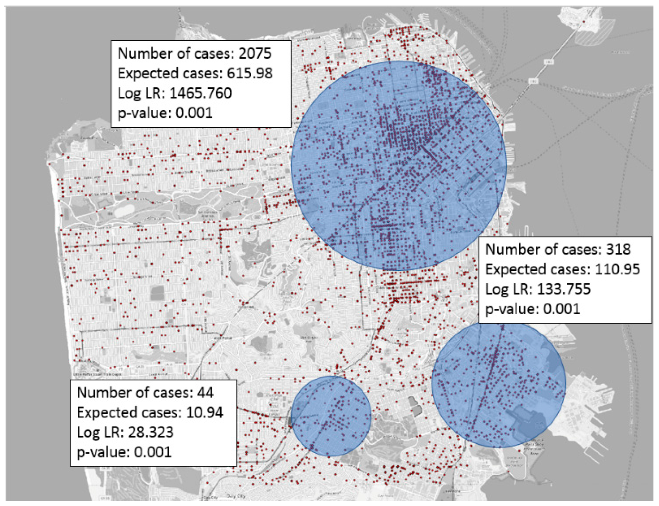
In classic data mining [26,27], most density-based clustering (e.g., K-means, DB-Scan [28]) approaches do not consider statistical significance. For example, K-means will always find several clusters or hotspots even though data points may follow a pure random (e.g., homogeneous Poisson process) or uniform distribution. In other words, traditional density-based clustering methods will generally output chance patterns if applied to geospatial hotspot detection. In contrast, methods that test for statistical significance (e.g. likelihood ratio based p-value test) can potentially reduce such chance patterns. For example, SaTScan [20,21] is one of the most well-known applications of significant hotspot detection. Figure 1 shows an example SaTScan output. The method uses hypothesis generation and ranking to enumerate possible hotspots, and ranks candidates based on a likelihood ratio. A statistical significance test is then used to remove chance hotspots based on their p-values. However, as stated in [7], a statistical test with a p-value alone may not be enough to reduce chance patterns. Thus, outputs from SaTScan may still contain false positives even though their p-value may pass the threshold (e.g., 0.01). In addition, if two randomly distributed points are close enough to each other, the circular hotspot generated by SaTScan using these two points can have an extremely high likelihood ratio, leading to a very small p-value which cannot be used to reject the null hypothesis using the current scheme. In fact, if we conceptually consider all possible circular regions (not limited to any algorithm-specific definition), we can always have very tiny circles containing only one point that have an unbounded likelihood ratio (assuming a continuous population distribution) even though they must be false positives. Since there is still possibility of such chance patterns, we need to strengthen the p-value based significance test with other measures as suggested in [8]. We may also consider some constraints on the size of the hotspot based on domain knowledge. Future work is still needed to improve the statistical rigor of hotspot detection to further reduce the number of chance patterns.
In addition to the traditional frequentist view of hotspot detection, which uses a randomization test (i.e., Monte Carlo Simulation) to evaluate statistical significance of results, Bayesian approaches have also been studied to identify emerging hotspots in spatiotemporal datasets. These methods capture the non-stationarity of data (e.g., change in number of disease incidents) and aims to find regions with a significant increase of events (e.g., disease, crime) [29,30].
2.3. Computer Science Foundation of Hotspot Detection
Geospatial hotspot detection is a computationally challenging task due to the volume of spatial big data such as large number of points or event instances (e.g., crime and disease locations) in input datasets. For example, in the U.S. there are around 10 million property crimes annually, and that is not counting the ever-increasing historical accumulation of these numbers. In addition, the enumerations are often challenging due to the large number of potential hotspot regions and the anti-monotonic properties of the interest measures (e.g., likelihood ratio) that are used for evaluation. For example, SaTScan uses a 2-point circle enumeration technique where one point is at the center and another is on the circumference of a circle, leading to a time complexity of O(N2), where N represents the number of points in the dataset. If we improve completeness by considering 3-point circles (i.e., three points on a circumference), this cost increases polynomially, i.e., O(N3). If we consider all possible circular regions for total completeness, the enumeration cost becomes exorbitant. Finally, for statistical significance testing, since the exact distribution of interest measure values (e.g., likelihood ratio) is unknown except for very simple density measures [23], a p-value often cannot be computed in close-form. Thus, Monte Carlo Simulation is commonly used in practice to simulate a null hypothesis through a large number of trials (e.g., 10,000), which requires repetitive execution of detection algorithms and multiplies the computational cost.
To improve the computational efficiency of geospatial hotspot detection, filter and refine strategies are often used to prune uninteresting candidates to save computational time. In Euclidean space, a ring-shaped hotspot detection method [19] uses a grid-based multi-resolution technique to quickly compute upper-bounds of the likelihood ratio on candidates during the prune phase, so the input threshold can be directly used to filter out candidates with an upper bound smaller than it. Rectangular hotspot detection [23] also uses a multi-resolution technique by decomposing each region into overlapping subsets. This approach guarantees an exact solution (i.e., identical output as a brute-force algorithm), and offers an option for approximated solutions, which exchange completeness for further speed-up. In the network space, linear hotspot discovery [4] implements dynamic segmentation which allows detection of hotspots at the sub-edge level on spatial networks while maintaining scalability. The algorithm also uses a filter-and-refine strategy (e.g., neighbor-node filtering, shortest path tree pruning) to reduce computational cost.
Parallel formulations have been proposed to speed up hotspot detection using GPU [31]. The Monte Carlo Simulation trials used to test statistical significance are also an embarrassingly parallel problem (e.g., one trial per node).
Unlike the frequentist approach above (i.e., finding persistent hotspots), the Bayesian spatial scan statistic [30] for emerging hotspot detection does not require Monte Carlo Simulation, reducing its execution time.
3. Foundations of Colocation Detection
Geospatial colocation patterns represent spatial features (e.g., geo-located objects or events) whose instances are often located together in a geographic neighborhood; such patterns are common in various domains and attract considerable research interest [32]. Colocation patterns often reflect symbiotic relationships, such as that between the Nile Crocodile and Egyptian Plover [33], which often reside in close proximity. Other biological dependencies (e.g., different types of blackberry canes) also have characteristics of colocation [34]. In climate change studies, colocation patterns between global plant growth and climate variables (e.g., precipitation) have also been found [35].
Unlike association rule mining [36] in classic data mining, which finds frequent subsets of items in a given set of transactions, colocation pattern detection has to handle spatial point distributions, where transactions do not naturally exist. To solve this problem, an event-centric model is widely used to build neighbor graphs to generate geospatial transactions [33].
3.1. Mathematical Foundation of Colocation Detection
Since distributions of spatial feature instances (e.g., trees, animals) do not naturally have transactions, as required in frequent pattern mining [36], mathematical models are needed to define transactions in geospatial datasets. A neighbor graph is one of the most common mathematical data representations used to form transactions using a spatial distribution of instances. In a neighbor graph, nodes are event instances, and edges are the relationships between them. A spatial relation (e.g., proximity) is used to convert a point distribution to a neighbor graph. For example, if we choose Euclidean distance to measure proximity between instances, then events of different feature types (e.g., a tree and a bird) are connected by edges in a neighbor graph if their Euclidean distance is smaller than a pre-defined threshold, which specifies the neighborhood size of interest. Whether the graph is directed or not depends on whether the spatial relation is symmetric (e.g., Euclidean distance is symmetric but network distance may not be). Because of the different metric spaces where the relation is defined, different neighbor graphs can be created. Commonly used spaces include Euclidean space, topological space, geographical space, and network space. Most of the methods for colocation pattern detection can be applied without considering the complex geographical context by treating the neighbor graph as an input.
Original definition for colocation detection [33] only applies to point events. To generalize the problem beyond point datasets, a buffer-based model was proposed to formulate colocation patterns of extended objects (e.g., polygons) [37]. In addition, while traditional colocation detection mainly focuses on global colocation patterns, some colocation patterns may only exist at a regional level (e.g., assault and drunk driving instances are co-located near bars), and recent approaches have targeted modeling such regional colocation patterns [38,39,40]. In this section, we will focus on colocation pattern detection using point objects.
3.2. Statistical Foundation of Colocation Detection
In order to detect the relationships between more than one feature of point events, spatial statistics uses the cross-K function, a generalization of Ripley’s K function for multivariate spatial point processes [41]. The cross-K function is defined as follows:
where i and j represents two types of instances (i.e., type i and type j), is the density (number per unit area) of type instances, is the distance, and is the expectation. When there are features, there would be cross-K functions for them, such as etc.
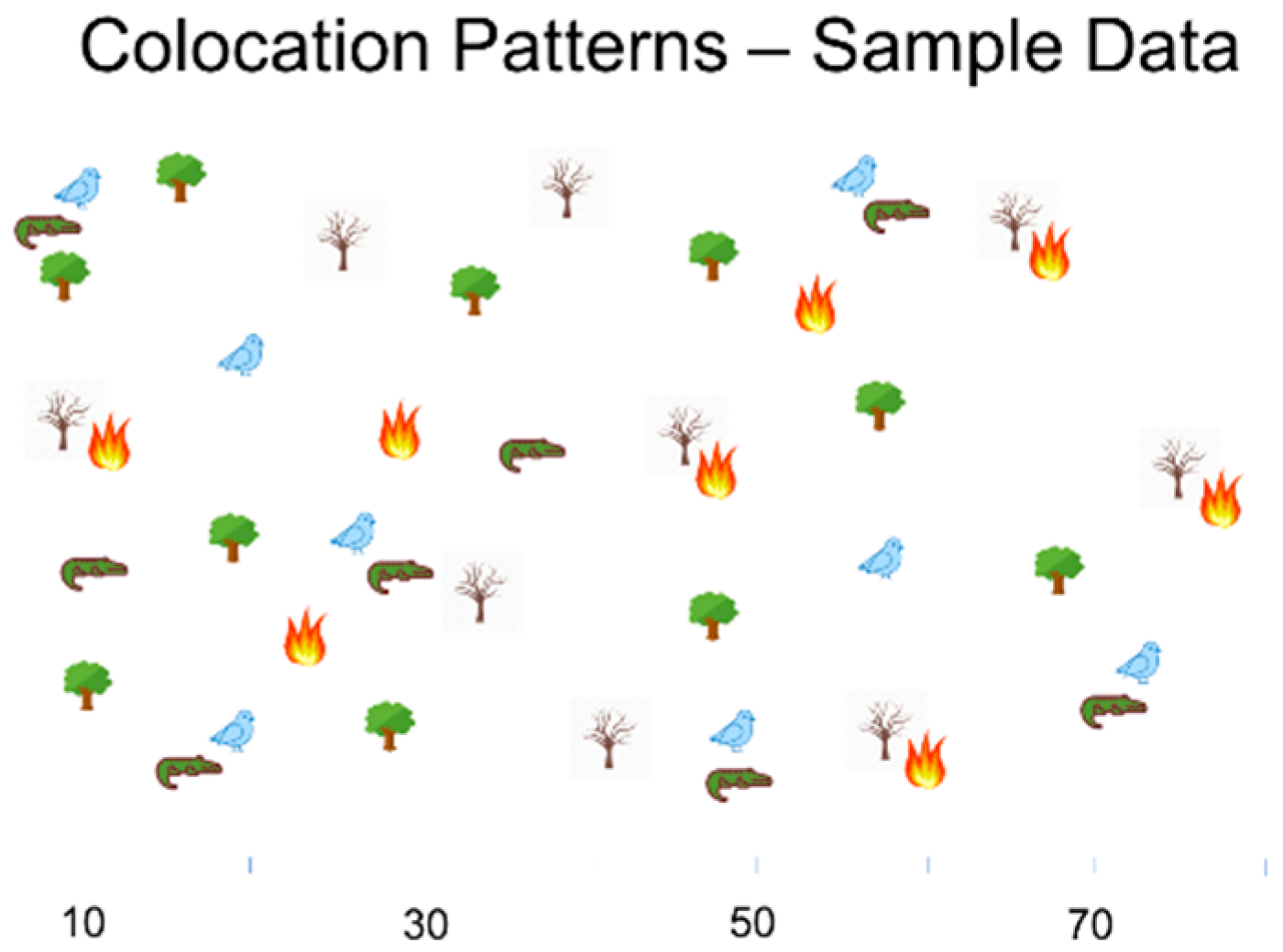
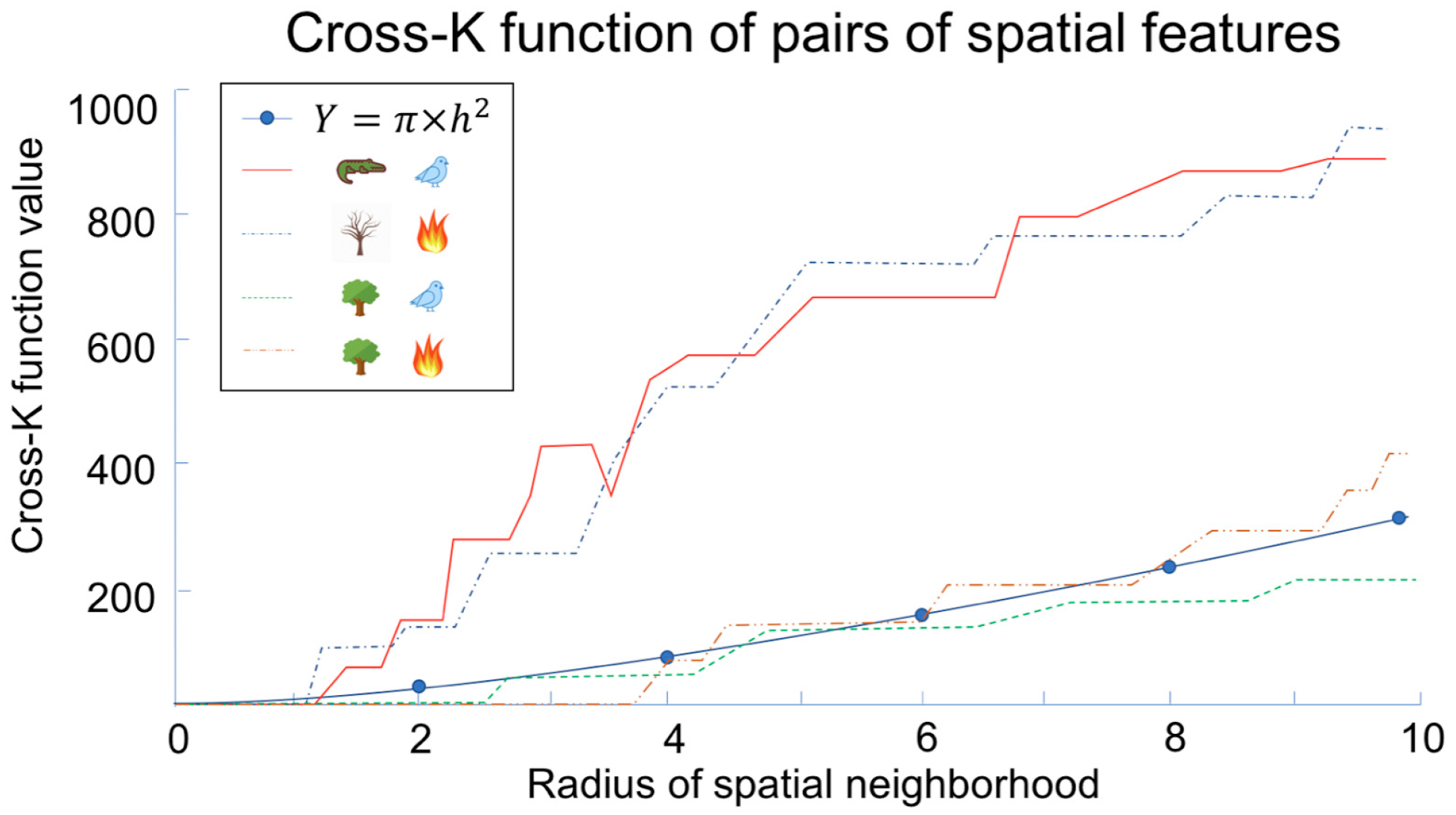
Figure 2 shows the spatial distribution of instances of five features, namely, plover, crocodile, green trees, dry trees, and wild fire, in a sample dataset. The pair-wise cross-K functions of four pairs are shown in Figure 3. The high cross-K function value shows features (i.e., wild fire and dry trees, plover and crocodile) that are more likely to locate near each other. By contrast, green trees with plovers and green trees with wild fire do not appear together commonly, as indicated by the corresponding low cross-K function values of these feature pairs.
Variations of the cross-K function, such as the L-function and the G function, are also used as interest measures to depict colocation patterns.
The participation index, an approximation of the cross-K function, is the most commonly used interest measure in colocation analysis. Before defining participation index, we need to first define participation ratio, another interest measure used inside the participation index. Given a colocation pattern and a feature within it, the participation ratio of in , , is the fraction of events of participating in any colocation instance of . A large value of indicates that events of tend to be located nearby other events of features in . Then, participation index () is defined as the minimal participation ratio of the features in a colocation pattern, that is . Participation index of two spatial features is an upper-bound on , where is the estimation of the cross-K function of colocation for a proximity neighborhood defined by distance [41], and is the total area of the region. In addition, given the instances of colocation pattern , and the instances of feature , we have enough information to compute .
Statistical significance test is used in colocation pattern detection to remove chance patterns [34]. Colocation pattern detection is concerned with the dependency between different spatial features, while the existence of autocorrelation between instances of the same feature may affect the value of the interest measure and result in colocation patterns detected by chance. For example, if clusters of two features’ instances are located nearby by chance, there will be lots of edges in the neighbor graph generated between these instances, leading to a colocation pattern. However, this pattern is more likely due to spatial autocorrelation and randomness instead of dependency between features. Statistical significance test can help evaluate the probability of a colocation pattern being detected by chance. Its null hypothesis assumes that different features are distributed in the space independently, while the alternative hypothesis is that the distribution is dependent. A spatial feature could be either spatially auto-correlated or not spatially auto-correlated. For example, to model an aggregated point patterns, a three-step Matern’s cluster process is applied: Step 1: A set of parent events is generated from a Poisson process with a constant intensity. Step 2: Each parent event is replaced by a random number of offspring points, where the number of points follows another Poisson distribution. Step 3: The offspring events are independently and identically distributed in a predefined neighborhood of their parent event.
3.3. Computer Science Foundation of Colocation Detection
Given a set of geospatial features, the number of combination of features grows exponentially as the number of features increases, making enumeration of colocation patterns computationally expensive.
To enumerate colocation patterns on spatial transactions, a join-based approach is commonly used to generate potential instances of patterns [42]. Based on this idea, a geometric approach [33] was proposed to reduce computational cost using spatial join algorithms and a combinatorial approach, which uses a sort-merge join strategy. Efforts have also been made to apply an Apriori algorithm [43] to colocation pattern detection. From a computational perspective, the participation index enjoys its nice property of monotonicity enjoys the advantage of having a nice monotonic property, that is, the index decreases monotonically as the size of the colocation pattern increases. If the participation index of a colocation pattern is less than a certain threshold, the index value for the patterns containing such a pattern must also be less than the threshold, and this can be used to eliminate un-interesting pattern candidates.
For large datasets without an available spatial index, a join-less approach can be employed [35]. Parallel formulations have been proposed to speed up colocation pattern detection using MapReduce [44]. There are also algorithms extending colocation pattern detection by considering dynamic neighborhoods of points [45].
4. Foundations of Spatial Prediction
Spatial prediction (i.e., spatial classification and regression) is the process of learning a model and predicting the target variable in a specific location using the training samples and the neighborhood relationship among the locations [46]. Spatial prediction is widely used by climate scientists, environmental specialists, land planners, etc. to identify different land cover types using remote sensing imagery, to detect changes in time as well as project future climate events. Spatial prediction is challenging due to specific properties of spatial datasets such as autocorrelation and heterogeneity [47]. Autocorrelation is the term that is used to describe the dependency between nearby samples. Heterogeneity describes the variation across different spatial locations [47].
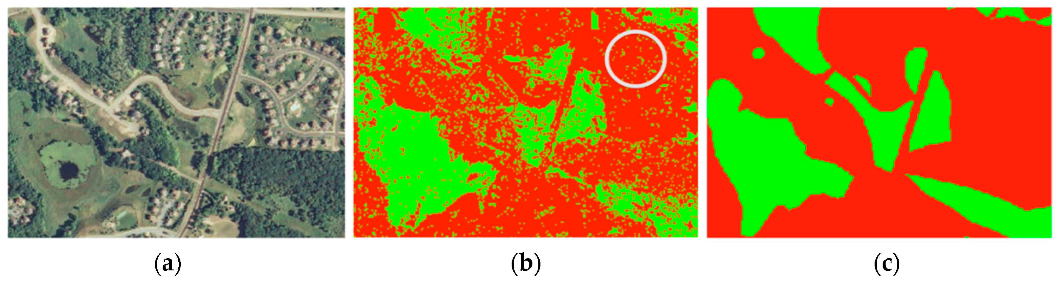
Traditional prediction approaches assume samples are drawn from an identical and independent distribution (i.i.d.). However, this assumption does not hold for spatial data, due to spatial autocorrelation and heterogeneity in the data, and using traditional tools for spatial prediction tasks may result in a large amount of prediction errors. For example, in Figure 4b, a decision tree approach is used to classify wet land and dry land using spectral features from a satellite image shown in Figure 4a. Compared to the ground truth in Figure 4c, the output of the decision tree contains a large amount of salt-and-pepper error due to limited consideration of spatial autocorrelation [6]. Note that focal-test-based spatial decision tree approaches, in which the tree traversal direction of a sample is based on both local and focal (i.e., neighborhood) information, can reduce such classification errors [6,48]. In spatial regression analysis, spatial properties are explicitly modeled to address spatial autocorrelation and heterogeneity. The spatial auto-regressive model (SAR) is a well-established model in this category. It predicts the dependent variables by considering the spatial relationships between independent variables, which requires a neighborhood relationship (often represented with the additional neighborhood matrix term ) as an additional input to investigate the effects of the location on the dependent variable. Similarly, there are approaches that incorporate spatial context into classification problems. For example, Markov Random Fields (MRF) provide a uniform framework for integrating spatial properties of the data and derive the probability distribution of interacting objects. Both SAR and MRF use identical models of spatial context for data.
Geographically Weighted Regression (GWR) [49] is another classic and widely used approach for modeling spatial auto-correlation. Instead of doing regression over all sample points, GWR uses only a subset of samples within a search window centered at the current location, and assigns more weights to closer samples during local regression.
This section discusses the three transdisciplinary foundations using spatial auto-regression (SAR) as an example. We’ve selected the SAR model for discussion here mainly based on our familiarity with it from previous research work [50,51]. Detailed analysis of GWR [49] and other models [52,53,54] will be examined in future work.
4.1. Mathematical Foundation of Spatial Prediction
The SAR model uses the spatial dependencies between different variables for prediction [55]. More specifically, given a spatial framework, a set of testing samples with dependent variables, a set of training samples as well as the neighborhood relationships (e.g., location information) among each data sample, SAR aims to find the optimal parameters for the model solution. To address the spatial dependencies, SAR explicitly includes spatial lag in its models: , where is a row-normalized neighborhood adjacency matrix, is the spatial auto-regression parameter (i.e., strength of the spatial dependency), is the matrix of observations of the explanatory variable, is the vector of regression coefficients, and represents the unobservable errors. Term is the autocorrelation term (or spatial lag), representing the spatial dependencies among the observations of dependent variable . As an extension of linear regression, SAR is more complex to solve due to the presence of the autocorrelation parameter () [50].
Spatial prediction is often associated with the optimization aspect of mathematics (e.g., minimize errors, maximize likelihood). In maximum likelihood based SAR, there are mainly two terms involved, a determinant term and a Sum of Square Error (SSE) term. These terms as well as the log likelihood function are uni-modular as proved in [55]. However, SAR parameter estimation requires extensive computational power due to the need for computing the determinant of a large matrix.
4.2. Statistical Foundation of Spatial Prediction
Bias and variance are two important aspects of spatial prediction. Bias is caused by erroneous assumptions in the prediction method. When the bias is high, the model is often considered as under-fitting. Similarly, variance is the sensitivity to the training dataset. In other words, if the model is perfectly fit (without considering the noisy training data and its effects on the model) to the training dataset, it may cause errors in the testing data due to over-fitting. As a model incorporates more parameters, and becomes more complex, bias decreases but the variance may cause more errors in the test dataset. For example, in linear regression, adding more terms to the model will increase the model complexity and thus increase variance and decrease bias.
A quick comparison with Markov Random Fields (MRF) sheds more light on elucidating the statistical foundations of SAR. For MRF, the posterior distribution is computed using Bayes’ rule, whereas in SAR, the posterior distribution is directly fitted to the data without a prior. In MRF, the relative frequencies are explicitly modeled in the class prior term. Thus, compared to Markov Random Fields, SAR makes more restrictive assumptions about the probability distributions as well as the class boundaries [46].
While SAR and MRF have been well studied to handle spatial datasets, many other learning or predicting algorithms require additional modeling to address the non-i.i.d. characteristics (e.g., spatial autocorrelation or heterogeneity) of geospatial data. For example, a focal-test based spatial decision tree was proposed to incorporate a focal autocorrelation statistic (e.g., focal Gamma index) into a traditional decision tree to reduce salt-and-pepper errors [6].
4.3. Computer Science Foundation of Spatial Prediction
Linear regression, the widely used traditional method in data mining for predicting numerically dependent variables, is considered to be a relatively inexpensive task computationally (e.g., solving linear least squares with normal equations, QR factorization, etc.). However, the method’s i.i.d. assumption ignores the unique spatial properties (e.g., autocorrelation) of geospatial data. SAR is able to model spatial dependencies using an autocorrelation term but that greatly increases its computational complexity due to the need for computing the determinant of a large matrix (i.e., ).
Both exact and approximate algorithms have been proposed to make SAR more efficient [50], [55]. Exact solutions, even with various algorithmic refinements [46,56] and parallelization strategies [51,57], may still suffer from high computational complexity and high memory cost (e.g., due to eigenvalues computation). Approximate solutions [58] aim to reduce complexity by providing reasonably good solutions (e.g., within a certain bound of the exact solution) instead of exact solutions. These methods include approximations based on Taylor’s series expansion [59], Chebyshev coefficients [60], and the Gauss-Lanczos algorithm [50]. MRF is computationally cheaper than SAR, and its computational cost can be further reduced by solving a suitable min-cut multi-way graph partitioning problem [61].
5. Foundations of Spatial Outlier Detection
Spatial outliers are spatial objects whose non-spatial attributes differ significantly from their spatial neighbors [62,63]. Spatial outliers are different from global outliers, which are detected based on the inconsistency between a set of observations and all other observations (i.e., they are likely to come from different distributions). A new house surrounded by older houses in a developed city can be considered as a spatial outlier, but it may not be a global outlier based on the overall house age.
Spatial outlier detection is critical in many applications such as suspicious object and behavior detection in criminology, anomalous traffic monitoring in transportation engineering, and fraud detection and prediction in credit card transactions.
5.1. Mathematical Foundation of Spatial Outlier Detection
The determination of a spatial outlier largely depends on the model of spatial proximity used. One straightforward way is to use Euclidean distance. This works well for objects or phenomena that generally have no obstacles between them. For example, Euclidean distance is the proper proximity measure for studying if the precipitation in a region is different from its neighbors. However, more factors need to be taken into account in other scenarios. When we conduct outlier detection on traffic data, distance on transportation networks is a much more accurate approximation. When we deal with data under a jurisdiction boundary such as county level aggregated disease mortality data, the proximity could be defined simply by the Euclidean distance between the centroid of each county. However, this assumes homogeneity within each county, which is not always true. Also, the objects located on two sides of a boundary can be largely different since objects within a county are assumed to be identical to those at the center of the county, which ignores spatial autocorrelation. For example, the data on different sides of a boundary are considered to belong to two different counties. A method to mitigate these negative effects and improve the modeling accuracy is to increase the resolution of aggregate data by allocating them into census blocks based on the population distribution. A spatial proximity relationship can be modeled by a neighbor graph in which a node represents an object and an edge represents the proximity between its two end nodes.
5.2. Statistical Foundation of Spatial Outlier Detection
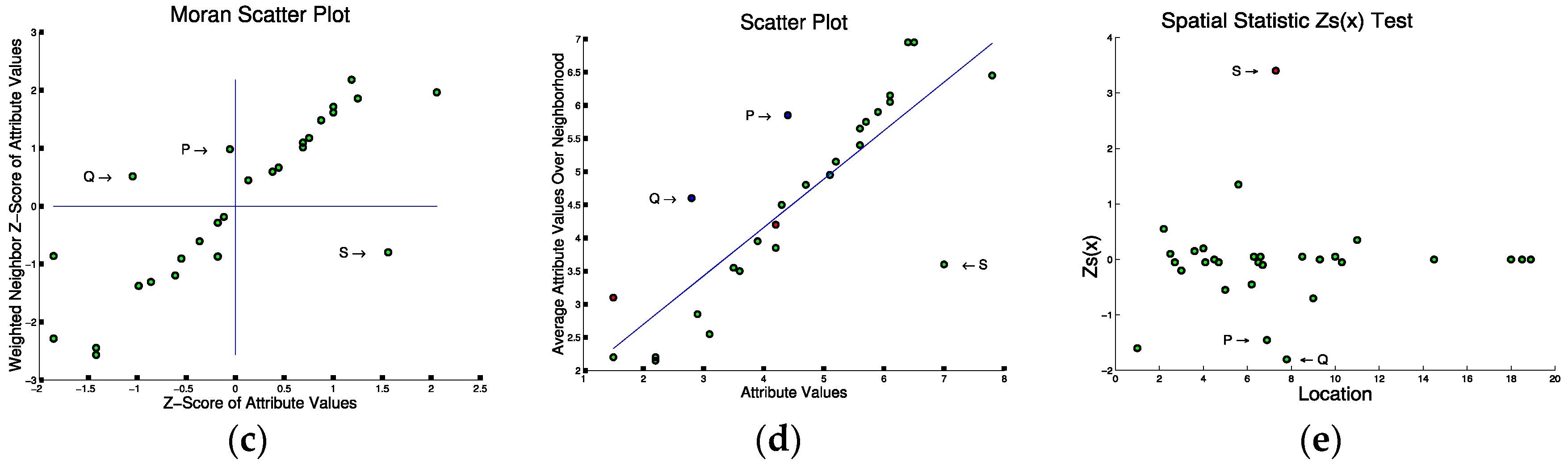
Statistical tests for spatial outliers fall into two categories: graphical tests (e.g. variogram clouds [64] and Moran scatterplots [65]) and quantitative tests (e.g. scatter plots [66] and neighborhood spatial statistics [62]). Graphical tests identify outliers by observing the visual pattern derived. Outliers usually stay either relatively far from the other points or inside specific regions such as certain quadrants. Figure 5 illustrates different testing methods for the 1-D input data in Figure 5a. The variogram cloud shown in Figure 5b finds two pairs of points (Q,S) and (P,S) that are apart from the cluster of remaining points, each pair representing spatially close points with significantly different non-spatial attribute values. The same points are detected by the Moran Scatter plot as shown in Figure 5c where the points in the upper-left and lower-right quadrants indicate points that are significant from their spatial neighbors. Quantitative tests identify outliers by measuring the difference between the investigated points’ non-spatial attributes and their spatial neighbors. Outliers are identified when the difference is larger than a threshold. In Figure 5d, the same points are detected far from the regression line by the scatter plot. Finally, a spatial statistic which measures the extent of the non-spatial difference from each point to its spatial neighbors also gives the same results from the overall score as shown in Figure 5e. Thus, all three approaches find points P, Q, and S to be of interest. From Figure 5a, we can see that S is a spatial outlier as it is far from its spatial neighbor P and Q.
5.3. Computer Science Foundation of Spatial Outlier Detection
A computer science framework for detecting a spatial outlier begins by defining a spatial neighborhood such as the region within a radius of Euclidian distance or network distance or region that has high topological connectivity. Then, it computes a test statistic which indicates how different the current location is compared to the other locations within the neighborhood in terms of non-spatial attributes [62]. A basic fundamental computational framework is illustrated in [62]. However, several challenges need to be addressed when outlier detection is applied on real-world problems. When there are multiple non-spatial attributes, defining the difference that incorporates all the attributes is difficult. Another challenge comes from how to define a neighborhood. Using a homogenous definition of neighbor area does not perform well given the heterogeneity of the large area it resides in. However, using a heterogeneous neighbor definition brings in significantly more computational cost. The irregular shape of a neighbor area also causes computational challenge. For example, computing the sum of a neighbor over an irregular shape is much costlier than over a rectangular area. Another challenge comes from the size of datasets. With the increased resolution of remote sensing imagery, raster data volumes are becoming larger and larger. In addition, each cell in the raster data is associated with a time-series of non-spatial attributes, which also multiplies the size of the dataset.
Recent computational research on spatial outlier detection falls into several categories. First, there are approaches that measure the occurrence of categorical attributes [67], overcoming the limitation that non-spatial attributes need to be numerical. Another approach combines multiple non-spatial attributes to a comprehensive outlier score [68]. Outlier detection has also been extended to flow anomaly detection, which finds outliers among time series in multiple locations. The key computational challenge is to identify the dominant intervals due to the lack of both monotonicity and optimal substructure in statistics of different time intervals, which disallows the use of Apriori-based and dynamic programming-based approaches. One solution to this problem is efficient window enumeration [69], which investigates algebraic properties. Finally, another popular direction is trajectory outlier detection [70,71], which identifies either trajectories that are significantly different from other trajectories [72] going through the same region or segments in a trajectory that are different from the rest of the trajectory [73,74,75]. The main challenge of trajectory outlier detection comes from the high dimensionality of trajectory data that is recorded in high frequency (e.g., one GPS record per second). Efficient computational schemes have been proposed [71,72] based on investigating the continuity of moving objects, which tend to have a momentum on their current direction and speed [70]. Thus, the trajectory data can be summarized by “change points” between which the trajectory keeps the same speed and direction.
6. Foundations of Teleconnection Discovery
Given a collection of spatial time series at different locations, teleconnection discovery aims to identify pairs of significant positively or negatively correlated spatial time series at large distances [47]. Teleconnection patterns are important in understanding the variability in climate through the discovery of pressure dipoles which are known to impact precipitation and temperature anomalies in the world [76]. Atmospheric pressure dipoles represent long distance connections between pressure anomalies of two distant regions that are negatively correlated with each other. Examples of pressure dipoles include the North Atlantic Oscillation which captures atmospheric fluctuations between Greenland and northern Europe, and the Southern Oscillation which captures pressure fluctuations between Tahiti and Darwin, Australia and corresponds to the well-known “El-Nino” effect (i.e., El-Nino Southern Oscillation). Computational challenges of teleconnection discovery include the large number of candidate pairs and the length of the time series. Another challenge is the large number of spurious high correlation patterns (i.e., false positives) that can occur. These challenges are addressed through a combination of mathematical, statistical and computer science approaches as discussed next.
6.1. Mathematical Foundation of Teleconnection Discovery
To address the challenge of the large number of candidate pairs, upper bounding techniques (Appendix A.1) have been proposed to allow pruning of uninteresting patterns [77,78]. First, a multi-dimensional unit sphere representation of the time series is used where the correlation of a pair of a time series is related to the cosine of the angle between their unit vector representations in the unit sphere. A cone representation is then used to represent a set of time series in the multi-dimensional unit sphere, and is characterized by two parameters: the center of the cone, and the span representing the maximal angle between any time series in the cone and the cone center. In [78], it was proved that if the smallest and largest angle between two cones are within a specific range then the correlation of any pair of time series from the two cones will be above (or below) the minimal required correlation threshold. These bounding conditions allow a more efficient traversal of the candidate pairs search space as discussed later in the computer science section (Section 6.3).
6.2. Statistical Foundation of Teleconnection Discovery
Statistics plays an essential role in teleconnection discovery since the pattern definition relies on a correlation measure, namely the Pearson correlation, for measuring the similarity between a pair of time series. To avoid spurious or false positive patterns, statistical significant tests have been proposed using a frequentist approach to identify statistically significant teleconnection patterns from climate data [79]. Challenges of significance testing include the underlying assumption of randomization tests that the data has i.i.d. As noted previously, this assumption does not hold for spatio-temporal data due it its high spatial and temporal autocorrelation. Another challenge is that the data is influenced by seasonality and trends that can impact the time series, leading to type I or type II errors. A third challenge is how to generate random samples under the null hypothesis in a way that is as close as possible to the true data generating process of the observed data. The null hypothesis in this case would be that the teleconnection pattern is spurious or uninteresting. Table 1 shows the approaches used to address each of these challenges as proposed in [79].
6.3. Computer Science Foundation of Teleconnection
As discussed earlier, discovering teleconnection patterns is a computationally challenging task due to the large number of time series pairs to be considered as well as the length of the time series. To efficiently identify these patterns, a filter and refine approach was proposed [77,78]. Given the upper and lower bound conditions on the smallest and largest angle between two cones [78] (the mathematical definition discussed in Section 7.1), cone-pairs can be classified into three categories: (a) those where all time series satisfy the correlation threshold (i.e., All-True), (b) those where no time series satisfies the correlation threshold (i.e., All-False), and (c) those which may have mixed time series. To reduce the number of time series pairs to be considered, an efficient cone-tree index structure was proposed where the spatial autocorrelation of nearby spatial time series is used to filter out redundant correlation computations. The proposed tree is based on a quad-tree implementation with threaded leaves to allow sequential scanning of the data. A heuristic is used to bound the maximal span of any cone in the tree. Once the tree is built, all-time series that are highly correlated with a given time series can be identified by starting from the root of the tree and scanning a node’s children only when it fails both the All-True and All-False conditions. In addition, a time series in a node that satisfies the All-True condition will be output, while All-False condition nodes will be ignored.
In [76], a framework was proposed to allow the discovery of dynamic teleconnections where dipoles are defined by moving rather than fixed regions. The framework consists of two phases: In the network construction phase, nodes are used to represent the set of nodes on the globe grid and edges connect node pairs with highly correlated time series. This is followed by a dipole construction phase. Using a greedy approach, it starts by selecting the most negative correlation edge in the network, and gradually grows the region on each end of the dipole edge by including other nodes which are highly positively correlated with one end of the edge while also being highly negatively correlated with the other end. The algorithm continues finding dipoles by picking the next most negative edge until the graph becomes very sparse or the most negative edge falls below a threshold. To ensure that the regions on each end of the dipole are spatially contiguous, a community-based method was proposed for partitioning the network before running the dipole construction algorithm. The community detection algorithm, based on random walk, allows partitioning the network into smaller subsets of nodes to find regions containing nodes that are highly positively or negatively correlated and avoiding smaller non-contiguous locations.
7. Discussion
Through our analysis of the mathematical, statistical and computer science foundations of the five geospatial techniques (Section 2, Section 3, Section 4, Section 5 and Section 6), it is evident that each foundation is important and necessary for solving geospatial data science problems. Additionally, many of the foundational concepts (e.g., mathematical modeling, statistical significance, computational structure) can be broadly applied across not only the five geospatial techniques that we discussed, but also other geospatial techniques. Statistical significance testing, for example, has been considered in multiple geospatial data mining techniques (e.g., for detecting hotspots, colocations and teleconnections) to reduce chance patterns, but there are many other approaches that have not considered much about statistical robustness (e.g., cascading spatiotemporal pattern detection [80], change footprint pattern discovery [81], co-occurrence pattern detection [82]). Using the statistical concepts and examples provided (e.g., Section 2.2), null and alternative hypotheses can be designed to incorporate significance testing and strengthen these techniques.
Each of the geospatial techniques discussed here underwent a long development before many important concepts from mathematics, statistics and computer science were recognized and incorporated. Hotspot detection, for example, started with a focus on statistical rigor (e.g., use of likelihood ratio and significance testing) [20,21] but did not consider much about computational scalability and efficiency, whereas colocation detection first developed through many computational refinements [33] and later recognized the importance of statistical rigor [34]. This further emphasizes the importance of a transdisciplinary view of data science in the geospatial domain. By not working in silos, and instead, taking a more holistic view that integrates foundational concepts from all three disciplines simultaneously, researchers can greatly improve and speed up problem solving in the geospatial domain. Most importantly, without a transdisciplinary view or understanding of geospatial data science, it will remain difficult to correctly apply or interpret results from geospatial data mining or machine learning techniques. As noted earlier, without awareness of the statistical i.i.d. assumption used in many machine learning techniques (e.g., random forest), a direct application of such techniques may return results with a high volume of salt-and-pepper errors in auto-correlated geospatial datasets [6]. Thus, it is critical to keep the transdisciplinary foundations in mind when developing or applying data-driven geospatial techniques.
7.1. Gaps and Opportunities
With the transdisciplinary view of geospatial techniques, there are still many challenges and opportunities lying ahead.
From siloed foundations to transdisciplinary foundations: While the five examples of geospatial techniques have made developments in mathematics, statistics and computer science, there still exist many other techniques that are studied in siloed disciplines. For example, as we mentioned earlier, many techniques are strong in computational scalability and mathematical completeness but have not considered statistical robustness, including cascading spatiotemporal pattern detection [80], change footprint pattern discovery [81] and co-occurrence pattern detection [82]. In addition, many patterns can be well defined mathematically and statistically (e.g., linear hotspots as simple-paths between nodes on road segments) but have no efficient algorithms to enumerate them unless assumptions are simplified (e.g., shortest-paths as a simplification of all simple-paths). These techniques should be further strengthened by addressing their transdisciplinary limitations.
For current geospatial techniques that have considered all three transdisciplinary foundations (e.g., hotspot detection), there still exist major gaps that need to be addressed. Statistical robustness is one of the major concerns given its importance to many critical societal applications (e.g., alarm of disease outbreaks, crime pattern analysis).
Effect size: Although significance testing has been incorporated into many of the techniques, the test itself (e.g., p-value test) still offers limited insight into the patterns detected and has raised broad concerns in recent years [7,8]. For example, in hotspot detection, if a pattern (i.e., a hotspot region) is statistically significant based on the p-value threshold, we are confident that an individual inside the region is more likely to be affected by an event (e.g., the spread of a disease) than an individual outside. However, the p-value does not tell how much more likely it is (i.e., the effect size). If the effect size is in fact small, then domain experts may still consider the pattern as a false positive. Thus, there is still a need to further consider effect size beyond a p-value test.
Multiple significance testing: For pattern detection problems (e.g., hotspot, colocation, teleconnection), geospatial data mining techniques can be considered as methods of hypotheses generation and testing, that is, they often enumerate a large number of possible candidate patterns (e.g., geographic regions in hotspot detection) and then conduct significance tests on them. When the total number of significant tests is large, although each single significant result may have a low probability of being false (e.g., 0.01 or 0.05 depending on the p-value threshold), the probability of all of them being true can be very low. Thus, the technique of multiple significance testing [83] can be introduced to mitigate this issue. For example, the p-value threshold for each individual test can be made smaller to maintain a good overall performance. Lowering p-value threshold (i.e., type-I error), however, could lead to lower statistical power (i.e., higher type-II error) [84] and this will consequently require more data to improve the power. Such issues have yet to be well addressed in geospatial pattern mining.
Additionally, beyond the scope of this paper, opportunities exist to further improve the understanding of transdisciplinary foundations for a broader set of models, including spatiotemporal techniques and simulation models.
Spatiotemporal techniques: Besides space, time is another important dimension that is frequently related to geospatial problems [85,86,87,88,89], and many geospatial techniques have been expanded to enable spatiotemporal analysis (e.g., Bayesian spatial scan statistics [30], cascading spatiotemporal pattern [80]). Adding temporal aspects into geospatial problems may require new mathematical modeling (e.g., time-expanded graph [90]), spatiotemporal statistics [85] and more complex computational structures.
Simulation models: Simulation models based on physical rules (e.g., the Soil and Water Assessment Tool [91], flood and solar simulation [92,93]), as opposed to data-driven models, provide different perspectives on problem solving. These models are built using domain knowledge (e.g., soil and water physics) and can be compared with data-driven solutions. Due to the computational complexity of many simulation models, data science techniques have been applied to provide fast approximation of the solutions [94].
8. Conclusions
Geospatial data science is a transdisciplinary field with foundations in mathematics, statistics, and computer science. To provide concrete examples of how geospatial techniques can be examined through the lens of mathematics, statistics, and computer science, we presented case studies on five geospatial techniques, namely hotspot detection, colocation detection, prediction, outlier detection and teleconnection detection. Many of the foundational concepts (e.g., statistical robustness) discussed in the five specific case studies can be broadly applied to other geospatial techniques. Through the case studies on five geospatial techniques, we showed that it is important to understand the transdisciplinary foundations (e.g., concepts, assumptions) in order to appropriately develop and apply geospatial techniques.
Gaps and opportunities: While lots of developments have been made to strengthen geospatial techniques, two major gaps need to be addressed as detailed in Section 7.1. First, many techniques are still studied within siloed disciplines and have not considered issues in the others. Second, statistical robustness of existing techniques must be further strengthened by considering effect size and multiple significance testing. Filling these gaps will lead to great opportunities in sectoral applications (e.g., robust prediction of disease outbreak with improvements in hotspot detection).
In future work, we will first study the transdisciplinary data science foundations of more geospatial techniques, identify their limitations and address them (e.g., spatially-constrained optimization [95,96], detection of co-occurrence patterns [82] and trajectory patterns [71,97], evacuation planning [98] and change detection [81,99]). Second, we will extend our scope to investigate the foundations of spatiotemporal techniques and simulation models. Third, we will further improve the current understanding and robustness of data science foundations of the techniques studied in this paper (e.g., maturing significance test as discussed in Section 7.1).
Acknowledgments
This material is based upon work supported by the National Science Foundation under Grants No. 1541876, 1029711, IIS-1320580, 0940818 and IIS-1218168, the USDOD under Grants No. HM1582-08-1-0017 and HM0210-13-1-0005, ARPA-E under Grant No. DE-AR0000795, USDA under Grant No. 2017-51181-27222 and the OVPR Infrastructure Investment Initiative and Minnesota Supercomputing Institute (MSI) at the University of Minnesota. We also thank Kim Koffolt and Jayant Gupta for improving the readability of this article.
Author Contributions
Yiqun Xie and Shashi Shekhar organized the paper structure. Yiqun Xie wrote the Introduction (Section 1), Transdisciplinary Foundations (Appendix A), Discussion (Section 7) and Conclusion (Section 8), and coordinated and integrated all other sections. Yiqun Xie, Emre Eftelioglu, and Ruhi Doshi summarized hotspot foundations (Section 2). Yan Li and Yiqun Xie summarized colocation foundations (Section 3). Emre Eftelioglu summarized prediction foundations (Section 4). Xun Tang summarized outlier foundations (Section 5). R.A. summarized teleconnection foundations (Section 6).
Conflicts of Interest
The authors declare no conflict of interest.
Appendix A. Transdisciplinary Foundations: Mathematics, Statistics and Computer Science
This appendix provides a broader set of important concepts in mathematics, statistics and computer science to consider in geospatial data science research (not limited to the techniques discussed in this paper). More details are also provided for the common concepts that are briefly discussed in Section 1.2.
A.1. Mathematics
Data representation: Mathematics provides powerful and succinct tools for data representation (e.g., matrix theory, graph theory). In pattern mining, these tools can be used to precisely define a pattern (e.g., a set of parameters needed to uniquely identify a pattern instance) and its search space (e.g., a parameter space of all possible parameter values). Based on the data representations, specialized analytics can be used to explore the properties of data and improve data quality (e.g., principle component analysis). In the geospatial domain, some traditional mathematical data models need to be extended to handle spatial dataset. For example, graph models in mathematics do not intrinsically have the capacity to model turns in road networks (e.g., the wait time for left turns and right turns is different) or non-stationary properties (e.g., travel time of edges is longer during rush hours). These issues call for additional modeling (e.g., time-expanded graphs).
Bounds: Upper and lower bounds are often used to narrow down the search space of a candidate pattern or provide guarantee on solution quality. When a search space is very large, non-smooth or non-convex, it is very challenging to efficiently enumerate through the search space (e.g., gradient descent). In this case, upper and lower bounds of solutions at unsearched places can be derived and compared with existing solutions to reduce the number of candidates. Monotonicity is often very helpful to derive tight bounds. When an optimal solution cannot be guaranteed, upper bound and lower bound analysis can provide meaningful insights to understand solution quality.
Completeness and correctness: Completeness guarantees all choices (e.g., combinatorial combinations of parameters) in the search space have been evaluated or the unevaluated ones are strictly bounded by the current best choices. Correctness comes with constraints (e.g., likelihood ratio or p-value threshold). Analysis should be performed to prove solutions do not violate any of the constraints.
Optimization: Optimization (both constrained and unconstrained) is commonly used in geospatial data science (e.g., parameter estimation in prediction). Appropriate use of optimization methods (e.g., gradient descent) should include discussions on properties of smoothness, convexity, convergence, global optimality (e.g., global vs. local optimality), etc.
A.2. Statistics
Traditional statistics vs. spatial statistics: Many core theories in statistics (e.g., central limit theorem) assume that data points have identical and independent distribution (i.i.d.). The i.i.d. assumption does not hold, however, for geospatial data analysis. As stated by Tobler’s first law of Geography: “Everything is related to everything else, but nearby things are more related than distant things” [100]; geospatial objects are not independent on each other. This fundamental difference gave rise to spatial statistics, which explicitly deals with spatial autocorrelation and spatial heterogeneity. In addition, the issue of anisotropy also needs to be considered. Tools of spatial statistics [101] include geostatistics (e.g., variograms, Kriging) for point-reference data analysis, spatial point processes (e.g., complete spatial randomness, Matern cluster process) for point distribution analysis, and lattice statistics (e.g., Moran’I, simultaneous autoregressive model, conditional autoregressive model) for discrete data analysis (e.g., raster).
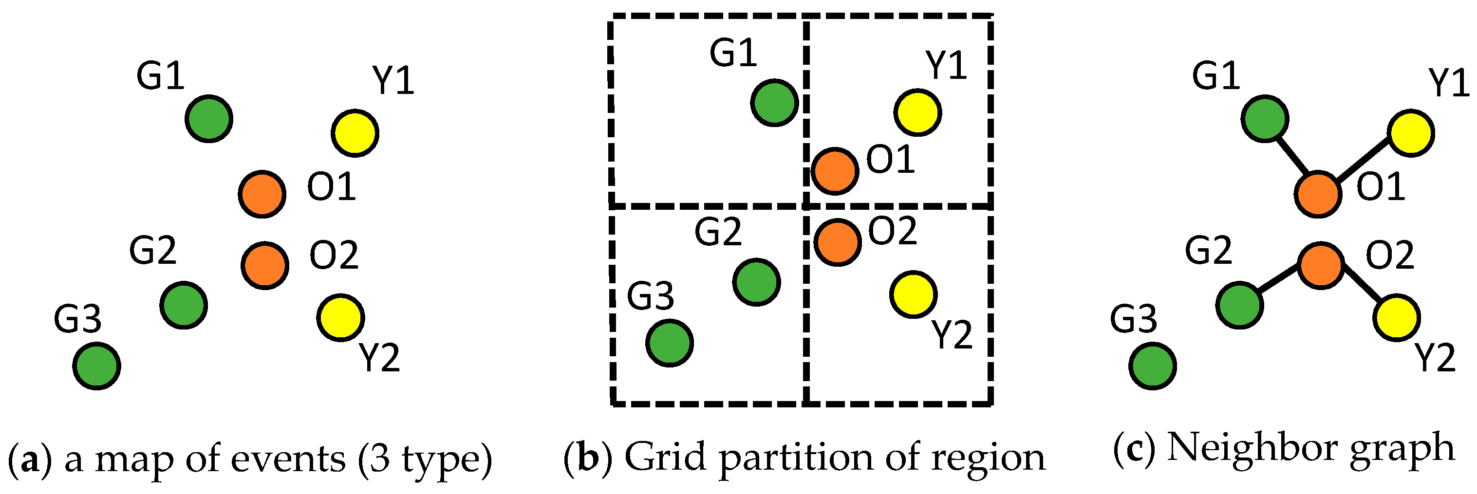
When applied to geospatial datasets, traditional statistics needs to be reconsidered to handle the spatial relationships among data points. The example in Figure A1a shows a distribution of three types of events. There are three instances of green, two of orange and two of yellow. In order to apply Pearson’s correlation analysis on event types, a natural pre-processing step is to partition the study area as shown in Figure A1b (i.e., to make sure that each event can be modeled using a fixed length of parameters). The four grid cells in Figure A1b are ordered as follows: top-left, bottom-left, top-right and bottom right [9]. Then, to represent each event type, we can use a vector of length four to store the number of instances of each type in each grid cell. For example, the green type event has one instance in the top left cell, two in bottom-left, and zeros in top-right and bottom-right, so its vector representation is [1, 2, 0, 0]. Similarly, the vector representation of orange is [0, 0, 1, 1] and yellow, [0, 0, 1, 1].
Figure A1.
Example of spatial statistics. (a) Shows distribution of three types of events colored in green, orange and yellow. (b) Shows a grid partition that splits original study area into four cells. (c) Shows a neighbor graph generated based on point distribution in (a).
Figure A1.
Example of spatial statistics. (a) Shows distribution of three types of events colored in green, orange and yellow. (b) Shows a grid partition that splits original study area into four cells. (c) Shows a neighbor graph generated based on point distribution in (a).

For event pairs (orange, green) and (orange, yellow), Table A1 shows their Pearson’s correlation coefficients and participation index [33] values (computed using neighbor graph in Figure A1c). Although orange instances are close to both yellow and green instances, Pearson’s correlation values indicated opposite relationships (i.e., negative vs. positive) between the two pairs of events. This unexpected result is caused by the space partitioning, whose boundaries break the adjacency between orange and green instance. In contrast, with spatial neighbor graph [33], participation index correctly captures both adjacencies of (orange, green) and (orange, yellow). This example shows the importance of spatial modeling when statistics is applied to geospatial dataset.

Table A1.
Pearson’s correlation coefficient and participation index for two event pairs.
| Event Pairs | Pearson’s Correlation Coefficient | Participation Index |
|---|---|---|
| (Green, Orange) | −0.90 | 0.67 |
| (Yellow, Orange) | 1 | 1 |
Frequentist vs. Bayesian: Frequentist and Bayesian are two different views on parameter estimation. Frequentist approaches assume parameter values are stationary and can be accurately estimated with a sufficiently large number of observations. In contrast, Bayesian methods assume a prior distribution of parameters, making their real values not fixed. As more data samples are collected, the new data is used to update the prior distribution, which captures the change of parameter values over time. Compared to the Frequentist approaches, Bayesian methods require a correct prior distribution.
Significance test: In a real-world scenario, we often have to deal with incomplete observations so the analysis will always be associated with some uncertainty. Frequentist approaches address this issue with a confidence interval to test the confidence on the analysis. In addition, we can evaluate how well a pattern conforms to the assumptions of the null hypothesis using a p-value test. We are more confident about the alternative hypothesis if the pattern is less likely to be generated from the null hypothesis. However, it is important to note that a p-value itself may not be sufficient to confirm a pattern or relationship (e.g., it does not show the size of the effect) [7,8]. In Bayesian statistics, predictions rely on Bayes Rule and the outputs directly give a posterior probability, so a separate significance test is not needed.
A.3. Computer Science
Hardness of problem: Before the design of an algorithm, the hardness of a given problem should be studied to narrow down the goal of the algorithm. For example, if a problem is NP-hard, then finding a polynomial time exact algorithm that guarantees solution optimality is as difficult as solving the “P versus NP” problem, which is one of the seven Millennium Prize Problems [102]. If the goal of the research is not to solve such a difficult theoretical problem, then it is more appropriate to find approximation or heuristic algorithms to solve the problem. In some cases, the solution of a problem can even be NP-hard to approximate within some constant ratios (e.g., APX-hard, NPO-complete) [103]. In such cases, designing problem-specific heuristic algorithms or adopting meta-heuristic algorithms (e.g., genetic algorithm, simulated annealing) might be a preferred choice. However, without hardness analysis, finding a heuristic solution rather than an optimal solution cannot be well justified.
Data structure and algorithm design paradigms: Based on the structure of the geospatial problems (e.g., point search, combinatorial enumeration), appropriate data structures (e.g., variations of trees and graphs) and algorithm design paradigms (e.g., dynamic programming, divide and conquer, greedy) can be selected to reduce computational cost. Note that a greedy algorithm is different from a heuristic algorithm. A greedy algorithm has two key properties, namely a greedy-choice property and an optimal substructure property, which together guarantee global optimality [104]. Heuristic algorithms generally have no guarantee on solution quality although they may use a greedy choice at a local step (e.g., decision tree). For optimization problems in prediction, gradient descent approaches are commonly applied to find either global or local optimum. In such problems, a variety of strategies exist to improve computational efficiency, including choices of descent direction (e.g., conjugate gradient descent), step size (e.g., Armijo rule) and batch size (e.g., stochastic gradient descent), as well as other acceleration techniques (e.g., Nesterov’s optimal first order method). For more difficult problems (e.g., non-differentiable, constrained cases), algorithms (e.g., ADMM, proximal gradient descent, projected gradient descent) should be chosen appropriately based on specific problem properties. Parallelization and high performance computing platforms (e.g., CyberGIS [105]) should also be considered to reduce computational cost. Especially, some algorithms may run slowly on a single core, yet perform very well once being parallelized (e.g., embarrassingly parallel). Dedicated parallel computing formulations have been proposed to accelerate algorithms on geospatial dataset [86].
Asymptotic complexity analysis: Space and time complexity is a direct indicator of the scalability of an approach and thus need to be carefully analyzed. Computer science provides a variety set of theories to analyze algorithm complexity, including Big O (upper bound), Theta (tight bound) and Omega complexity (lower bound), as well as amortized analysis (e.g., accountant method) [104]. In cases where time complexity varies significantly across problem instances (e.g., filter and refine algorithms), average time complexity or best/worst case scenarios can be analyzed to evaluate performance. For optimization problems, iteration complexity (or convergence rate) should be analyzed.
References
- Castelvecchi, D. Can we open the black box of AI? Nature 2016, 538, 20–23. [Google Scholar] [CrossRef] [PubMed]
- Kang, J.M.; Edwards, D.L. Tipping Points, Butterflies, and Black Swans: A Vision for Spatio-temporal Data Mining Analysis. In Advances in Spatial and Temporal Databases (SSTD-11); Springer: Berlin/Heidelberg, Germany, 2011; pp. 454–457. [Google Scholar]
- Institue for Mathematics and Its Applications. Transdisciplinary Foundations of Data Science [Online]. Available online: https://www.ima.umn.edu/2016-2017/SW9.14-16.16 (accessed on 4 November 2017).
- Kaiser, M.S.; Cressie, N.; Lee, J. Spatial mixture models based on exponential family conditional distributions. Stat. Sin. 2002, 12, 449–474. [Google Scholar]
- Wasserman, L. Rise of the Machines. Available online: http://www.stat.cmu.edu/~larry/Wasserman.pdf (accessed on 18 September 2017).
- Jiang, Z.; Shekhar, S.; Zhou, X.; Knight, J.; Corcoran, J. Focal-Test-Based Spatial Decision Tree Learning. IEEE Trans. Knowl. Data Eng. 2015, 27, 1547–1559. [Google Scholar] [CrossRef]
- Baker, M. Statisticians issue warning over misuse of p values. Nature 2016, 531, 151. [Google Scholar] [CrossRef] [PubMed]
- American Statistical Association. Releases Statement on Statistical Significance and p-Values. Available online: http://www.amstat.org/asa/files/pdfs/P-ValueStatement.pdf (accessed on 18 September 2017).
- Eftelioglu, E.; Ali, R.; Tang, X.; Xie, Y.; Li, Y.; Shekhar, S. Spatial Data Science: An Interdisciplinary Approach. In Geospatial Data Science: Techniques and Applications, 1st ed.; Karimi, H.A., Karimi, B., Eds.; CRC Press: Boca Raton, FL, USA, 2017; ISBN 1138626449. [Google Scholar]
- Blaschke, T.; Merschdorf, H. Geographic Information Science as a Multidisciplinary and Multiparadigmatic Field. Cartogr. Geogr. Inf. Sci. 2014, 41, 196–213. [Google Scholar] [CrossRef]
- Dragiæeviæ, S.; Balram, S. Collaborative Geographic Information Systems and Science: A Transdisciplinary Evolution; IGI Global: Hershey, PA, USA, 2006. [Google Scholar]
- Gunasekera, R. Use of GIS for environmental impact assessment: An interdisciplinary approach. Interdiscip. Sci. Rev. 2004, 29, 37–48. [Google Scholar] [CrossRef]
- Wang, T. Interdisciplinary urban GIS for smart cities: Advancements and opportunities. Geo-Spat. Inf. Sci. 2013, 16, 25–34. [Google Scholar]
- Cromley, E.K.; McLafferty, S. GIS and Public Health; The Guilford Press: New York, NY, USA, 2012. [Google Scholar]
- Xie, Y.; Runck, B.C.; Shekhar, S.; Kne, L.; Mulla, D.; Jordan, N.; Wiringa, P. Collaborative Geodesign and Spatial Optimization for Fragmentation-Free Land Allocation. ISPRS Int. J. Geo-Inf. 2017, 6, 226. [Google Scholar] [CrossRef]
- Kulldorff, M.; Nagarwalla, N. Spatial disease clusters: Detection and inference. Stat. Med. 1995, 14, 799–810. [Google Scholar] [CrossRef] [PubMed]
- Openshaw, S.; Craft, A.W.; Charlton, M.; Birch, J.M. Investigation of leukaemia clusters by use of a Geographical Analysis Machine. Lancet 1988, 1, 272–273. [Google Scholar] [CrossRef]
- Eftelioglu, E.; Shekhar, S.; Oliver, D.; Zhou, X.; Evans, M.R.; Xie, Y.; Kang, J.M.; Laubscher, R.; Farah, C. Ring-Shaped Hotspot Detection: A Summary of Results. In Proceedings of the IEEE International Conference on Data Mining (ICDM), Shenzhen, China, 14–17 December 2014; pp. 815–820. [Google Scholar]
- Eftelioglu, E.; Shekhar, S.; Kang, J.M.; Farah, C.C. Ring-Shaped Hotspot Detection. IEEE Trans. Knowl. Data Eng. 2016, 28, 3367–3381. [Google Scholar] [CrossRef]
- Kulldorff, M. A spatial scan statistic. Commun. Stat. Theory Methods 1997, 26, 1481–1496. [Google Scholar] [CrossRef]
- Kulldorff, M. SaTScan User Guide. Available online: https://www.satscan.org/cgi-bin/satscan/register.pl/SaTScan_Users_Guide.pdf?todo=process_userguide_download (accessed on 18 September 2017).
- Kulldorff, M. Spatial scan statistics: Models, calculations, and applications. In Scan Statistics and Applications; Springer: Berlin, Germany, 1999; pp. 303–322. [Google Scholar]
- Neill, D.B.; Moore, A.W. Rapid Detection of Significant Spatial Clusters. In Proceedings of the ACM SIGKDD (KDD ’04), Seattle, WA, USA, 22–25 August 2004. [Google Scholar]
- Tang, X.; Eftelioglu, E.; Oliver, D.; Shekhar, S. Significant Linear Hotspot Discovery. IEEE Trans. Big Data 2017, 3, 140–153. [Google Scholar] [CrossRef]
- Eftelioglu, E.; Li, Y.; Tang, X.; Shekhar, S.; Kang, J.M.; Farah, C. Mining Network Hotspots with Holes: A Summary of Results. In Proceedings of the International Conference on Geographic Information Science, Montreal, QC, Canada, 27–30 September 2016; pp. 51–67. [Google Scholar]
- Tan, P.; Steinbach, M.; Kumar, V. Introduction to Data Mining, 1st ed.; Addison-Wesley Longman Publishing Co., Inc.: Boston, MA, USA, 2005. [Google Scholar]
- Han, J.; Kammber, M.; Pei, J. Data Mining—Concepts and Techniques; Elsevier: Amsterdam, The Netherlands, 2011. [Google Scholar]
- Ester, M.; Kriegel, H.-P.; Sander, J.; Xu, X. A Density-Based Algorithm for Discovering Clusters in Large Spatial Databases with Noise. In Proceedings of the Second International Conference on Knowledge Discovery and Data Mining (KDD ’96), Portland, OR, USA, 2–4 August 1996; pp. 226–231. [Google Scholar]
- Neill, D.B.; Moore, A.W.; Sabhnani, M.; Daniel, K. Detection of Emerging Space-Time Clusters. In Proceedings of the Eleventh ACM SIGKDD International Conference on Knowledge Discovery and Data Mining (KDD ’05), Chicago, IL, USA, 21–24 August 2005; pp. 218–227. [Google Scholar]
- Neill, D.B.; Moore, A.W.; Cooper, G.F. A Bayesian Spatial Scan Statistic. In Proceedings of the Neural Information Processing Systems Conference (NIPS), Vancouver, BC, Canada, 6–9 December 2005; pp. 1003–1010. [Google Scholar]
- Pang, L.X.; Chawla, S.; Scholz, B.; Wilcox, G. A Scalable Approach for LRT Computation in GPGPU Environments. In Proceedings of the 15th Asia-Pacific Web Conference (APWeb 2013), Sydney, Australia, 4–6 April 2013; pp. 595–608. [Google Scholar]
- Yoo, J.S.; Bow, M. Mining spatial colocation patterns: A different framework. Data Min. Knowl. Discov. 2012, 24, 159–194. [Google Scholar] [CrossRef]
- Huang, Y.; Shekhar, S.; Xiong, H. Discovering colocation patterns from spatial data sets: A general approach. IEEE Trans. Knowl. Data Eng. 2004, 16, 1472–1485. [Google Scholar] [CrossRef]
- Barua, S.; Sander, J. Mining Statistically Significant Co-location and Segregation Patterns. IEEE Trans. Knowl. Data Eng. 2014, 26, 1185–1199. [Google Scholar] [CrossRef]
- Yoo, J.S.; Shekhar, S. A joinless approach for mining spatial colocation patterns. IEEE Trans. Knowl. Data Eng. 2006, 18, 1323–1337. [Google Scholar]
- Hipp, J.; Güntzer, U.; Nakhaeizadeh, G. Algorithms for association rule mining—A general survey and comparison. ACM SIGKDD Explor. Newsl. 2000, 2, 58–64. [Google Scholar] [CrossRef]
- Xiong, H.; Shekhar, S.; Huang, Y.; Kumar, V.; Ma, X.; Yoc, J. A Framework for Discovering Co-location Patterns in Data Sets with Extended Spatial Objects. In Proceedings of the SIAM International Conference on Data Mining, Lake Buena Vista, FL, USA, 4–6 April 2004; pp. 78–89. [Google Scholar]
- Wang, S.; Huang, Y.; Wang, X.S. Regional Co-locations of Arbitrary Shapes. In Advances in Spatial and Temporal Databases, Proceedings of the 13th International Symposium, SSTD 2013, Munich, Germany, 21–23 August 2013; Springer: Berlin, Germany, 2013; pp. 19–37. [Google Scholar]
- Deng, M.; Cai, J.; Liu, Q.; He, Z.; Tang, J. Multi-level method for discovery of regional co-location patterns. Int. J. Geogr. Inf. Sci. 2017, 31, 1846–1870. [Google Scholar] [CrossRef]
- Eick, C.F.; Parmar, R.; Ding, W.; Stepinski, T.F.; Nicot, J.-P. Finding regional co-location patterns for sets of continuous variables in spatial datasets. In Proceedings of the 16th ACM SIGSPATIAL International Conference on Advances in Geographic Information Systems (GIS ’08), Irvine, CA, USA, 5–7 November 2008. [Google Scholar]
- Dixon, P.M. Ripley’s K Function. In Encyclopedia of Environmetrics; John Wiley & Sons, Ltd: Chichester, UK, 2002; pp. 1796–1803. [Google Scholar]
- Shekhar, S.; Huang, Y. Discovering Spatial Co-location Patterns: A Summary of Results. In Advances in Spatial and Temporal Databases, Proceedings of the 7th International Symposium, SSTD 2001, Redondo Beach, CA, USA, 12–15 July 2001; Springer: Berlin, Germany, 2001; pp. 236–256. [Google Scholar]
- Agrawal, R.; Srikant, R. Fast algorithms for mining association rules. In Proceedings of the 20th International Conference on Very Large Data Bases (VLDB), Santiago de Chile, Chile, 12–15 September 1994; pp. 487–499. [Google Scholar]
- Yoo, J.S.; Boulware, D.; Kimmey, D. A Parallel Spatial Co-location Mining Algorithm Based on MapReduce. In Proceedings of the 2014 IEEE International Congress on Big Data, Anchorage, AK, USA, 27 June–2 July 2014; pp. 25–31. [Google Scholar]
- Qian, F.; He, Q.; He, J. Mining spatial co-location patterns with dynamic neighborhood constraint. In Machine Learning and Knowledge Discovery in Databases, Proceedings of the European Conference (ECML PKDD 2009), Bled, Slovenia, 7–11 September 2009; Springer: Berlin, Germany, 2009; pp. 238–253. [Google Scholar]
- Shekhar, S.; Schrater, P.R.; Vatsavai, R.R.; Wu, W.; Chawla, S. Spatial contextual classification and prediction models for mining geospatial data. IEEE Trans. Multimed. 2002, 4, 174–188. [Google Scholar] [CrossRef]
- Shekhar, S.; Jiang, Z.; Ali, R.Y.; Eftelioglu, E.; Tang, X.; Gunturi, V.; Zhou, X. Spatiotemporal Data Mining: A Computational Perspective. ISPRS Int. J. Geo-Inf. 2015, 4, 2306–2338. [Google Scholar] [CrossRef]
- Fauvel, M.; Chanussot, J.; Benediktsson, J.A. A spatial–spectral kernel-based approach for the classification of remote-sensing images. Pattern Recognit. 2012, 45, 381–392. [Google Scholar] [CrossRef]
- Brunsdon, C.; Fotheringham, S.; Charlton, M. Geographically Weighted Regression. J. R. Stat. Soc. Ser. D 1998, 47, 431–443. [Google Scholar] [CrossRef]
- Celik, M.; Kazar, B.M.; Shekhar, S.; Boley, D.; Lilja, D.J. Spatial dependency modeling using spatial auto-regression. In Proceedings of the ICA Workshop on Geospatial Analysis and Modeling, Vienna, Austria, 8 July 2006; pp. 186–197. [Google Scholar]
- Kazar, B.M.; Shekhar, S.; Lilja, D.J.; Boley, D. A Parallel Formulation of the Spatial Auto-Regression Model for Mining Large Geo-Spatial Datasets. In Proceedings of the 2004 SIAM International Conference on Data Mining, Workshop on High Performance and Distributed Mining (HPDM 2004), Lake Buena Vista, FL, USA, 22–24 April 2004. [Google Scholar]
- Wall, M.M. A close look at the spatial structure implied by the CAR and SAR models. J. Stat. Plan. Inference 2004, 121, 311–324. [Google Scholar] [CrossRef]
- Griffith, D.A. A linear regression solution to the spatial autocorrelation problem. J. Geogr. Syst. 2000, 2, 141–156. [Google Scholar] [CrossRef]
- Gagliasso, D.; Hummel, S.; Temesgen, H. A Comparison of Selected Parametric and Non-Parametric Imputation Methods for Estimating Forest Biomass and Basal Area. Open J. For. 2014, 4, 42–48. [Google Scholar] [CrossRef]
- Celik, M.; Kazar, B.M.; Shashi, S.; Boley, D.; Lilja, D.J. A Parameter Estimation Method for the Spatial Autoregression Model. 2007. Available online: http://www-users.cs.umn.edu/~boley/publications/papers/NASA06.pdf (accessed on 18 September 2017).
- Pace, R.K.; LeSage, J.P. Closed-form maximum likelihood estimates for spatial problems. Geogr. Anal. 2000, 32, 154–172. [Google Scholar] [CrossRef]
- Li, B. Implementing spatial statistics on parallel computers. In Practical Handbook of Spatial Statistics; CRC Press: Boca Raton, FL, USA, 1996; pp. 107–148. [Google Scholar]
- Kazar, B.M.; Shekhar, S.; Lilja, D.J.; Vatsavai, R.R.; Pace, R.K. Comparing exact and approximate spatial auto-regression model solutions for spatial data analysis. In Proceedings of the International Conference on Geographic Information Science, Adelphi, MD, USA, 20–23 October 2004; pp. 140–161. [Google Scholar]
- Martin, R.J. Approximations to the determinant term in Gaussian maximum likelihood estimation of some spatial models. Commun. Stat. Methods 1992, 22, 189–205. [Google Scholar] [CrossRef]
- Pace, R.K.; LeSage, J.P. Chebyshev approximation of log-determinants of spatial weight matrices. Comput. Stat. Data Anal. 2004, 45, 179–196. [Google Scholar] [CrossRef]
- Kazar, B.M.; Celik, M. Spatial AutoRegression (SAR) Model; Springer: Boston, MA, USA, 2012. [Google Scholar]
- Shekhar, S.; Lu, C.T.; Zhang, P. A unified approach to detecting spatial outliers. Geoinformatica 2003, 7, 139–166. [Google Scholar] [CrossRef]
- Aggarwal, C.C. Outlier analysis. In Data mining; Springer: Berlin, Germany, 2015; pp. 237–263. [Google Scholar]
- Haslett, J.; Bradley, R.; Craig, P.; Unwin, A.; Wills, G. Dynamic graphics for exploring spatial data with application to locating global and local anomalies. Am. Stat. 1991, 45, 234–242. [Google Scholar]
- Anselin, L. Local indicators of spatial association—LISA. Geogr. Anal. 1995, 27, 93–115. [Google Scholar] [CrossRef]
- Anselin, L. Exploratory spatial data analysis and geographic information systems. New Tools Spat. Anal. 1994, 17, 45–54. [Google Scholar]
- Liu, X.; Chen, F.; Lu, C.-T. On detecting spatial categorical outliers. Geoinformatica 2014, 18, 501–536. [Google Scholar] [CrossRef]
- Chen, D.; Lu, C.-T.; Kou, Y.; Chen, F. On detecting spatial outliers. Geoinformatica 2008, 12, 455–475. [Google Scholar] [CrossRef]
- Kang, J.M.; Shekhar, S.; Wennen, C.; Novak, P. Discovering flow anomalies: A SWEET approach. In Proceedings of the 8th IEEE International Conference on Data Mining (ICDM), Pisa, Italy, 15–19 December 2008; pp. 851–856. [Google Scholar]
- Mazimpaka, J.D.; Timpf, S. Trajectory data mining: A review of methods and applications. J. Spat. Inf. Sci. 2016, 2016, 61–99. [Google Scholar] [CrossRef]
- Zheng, Y. Trajectory Data Mining. ACM Trans. Intell. Syst. Technol. 2015, 6, 1–41. [Google Scholar] [CrossRef]
- Kuang, W.; An, S.; Jiang, H. Detecting Traffic Anomalies in Urban Areas Using Taxi GPS Data. Math. Probl. Eng. 2015, 2015, 809582. [Google Scholar] [CrossRef]
- Lee, J.-G.; Han, J.; Li, X. Trajectory Outlier Detection: A Partition-and-Detect Framework. In Proceedings of the 24th IEEE International Conference on Data Engineering (ICDE), Cancun, Mexico, 7–12 April 2008; pp. 140–149. [Google Scholar]
- Liu, L.; Qiao, S.; Zhang, Y.; Hu, J. An efficient outlying trajectories mining approach based on relative distance. Int. J. Geogr. Inf. Sci. 2012, 26, 1789–1810. [Google Scholar] [CrossRef]
- Yuan, G.; Xia, S.; Zhang, L.; Zhou, Y.; Ji, C. Trajectory Outlier Detection Algorithm Based on Structural Features. J. Comput. Inf. Syst. 2011, 7, 4137–4144. [Google Scholar]
- Kawale, J.; Steinbach, M.; Kumar, V. Discovering dynamic dipoles in climate data. In Proceedings of the 2011 SIAM International Conference on Data Mining, Mesa, AZ, USA, 28–30 April 2011; pp. 107–118. [Google Scholar]
- Zhang, P.; Huang, Y.; Shekhar, S.; Kumar, V. Correlation analysis of spatial time series datasets: A filter-and-refine approach. In Proceedings of the Pacific-Asia Conference on Knowledge Discovery and Data Mining, Seoul, Korea, 30 April–2 May 2003; pp. 532–544. [Google Scholar]
- Zhang, P.; Huang, Y.; Shekhar, S.; Kumar, V. Exploiting spatial autocorrelation to efficiently process correlation-based similarity queries. In Advances in Spatial and Temporal Database, Proceedings of the 8th International Symposium, SSTD 2003, Santorini Island, Greece, 24–27 July 2003; Springer: Berlin, Germany; pp. 449–468.
- Kawale, J.; Chatterjee, S.; Ormsby, D.; Steinhaeuser, K.; Liess, S.; Kumar, V. Testing the significance of spatio-temporal teleconnection patterns. In Proceedings of the ACM SIGKDD (KDD ’12), Beijing, China, 12–16 August 2012; pp. 642–650. [Google Scholar]
- Mohan, P.; Shekhar, S.; Shine, J.A.; Rogers, J.P. Cascading Spatio-Temporal Pattern Discovery. IEEE Trans. Knowl. Data Eng. 2012, 24, 1977–1992. [Google Scholar] [CrossRef]
- Zhou, X.; Shekhar, S.; Mohan, P.; Liess, S.; Snyder, P.K. Discovering Interesting Sub-paths in Spatiotemporal Datasets: A Summary of Results. In Proceedings of the 19th ACM SIGSPATIAL International Conference on Advances in Geographic Information Systems (ACM SIGSPATIAL 2011), Chicago, IL, USA, 1–4 November 2011; pp. 44–53. [Google Scholar]
- Ali, R.Y.; Gunturi, V.M.V.; Kotz, A.J.; Shekhar, S.; Northrop, W.F. Discovering Non-compliant Window Co-Occurrence Patterns: A Summary of Results. In Advances in Spatial and Temporal Databases, Proceedings of the 14th International Symposium, SSTD 2015, Hong Kong, China, 26–28 August 2015; Springer: Berlin, Germany, 2015; pp. 391–410. [Google Scholar]
- Bland, J.M.; Altman, D.G. Multiple significance tests: The Bonferroni method. BMJ 1995, 310, 170. [Google Scholar] [CrossRef] [PubMed]
- Cohen, J. Statistical Power Analysis. Curr. Dir. Psychol. Sci. 1992, 1, 98–101. [Google Scholar] [CrossRef]
- Cressie, N.A.C.; Wikle, C.K. Statistics for Spatio-Temporal Data; Wiley: Hoboken, NJ, USA, 2011. [Google Scholar]
- Prasad, S.K.; Aghajarian, D.; McDermott, M.; Shah, D.; Mokbel, M.; Puri, S.; Rey, S.J.; Shekhar, S.; Xe, Y.; Vatsavai, R.R.; et al. Parallel Processing over Spatial-Temporal Datasets from Geo, Bio, Climate and Social Science Communities: A Research Roadmap. In Proceedings of the 2017 IEEE International Congress on Big Data (BigData Congress), Honolulu, HI, USA, 25–30 June 2017; pp. 232–250. [Google Scholar]
- Yu, H.; Shaw, S. Exploring potential human activities in physical and virtual spaces: A spatio-temporal GIS approach. Int. J. Geogr. Inf. Sci. 2008, 22, 409–430. [Google Scholar] [CrossRef]
- Gebbert, S.; Pebesma, E. TGRASS: A temporal GIS for field based environmental modeling. Environ. Model. Softw. 2014, 53, 1–12. [Google Scholar] [CrossRef]
- Evans, M.R.; Yang, K.S.; Kang, J.M.; Shekhar, S. A Lagrangian approach for storage of spatio-temporal network datasets: A summary of results. In Proceedings of the 18th SIGSPATIAL International Conference on Advances in Geographic Information Systems, San Jose, CA, USA, 3–5 November 2010; pp. 212–221. [Google Scholar]
- Köhler, E.; Langkau, K.; Skutella, M. Time-expanded graphs for flow-dependent transit times. In Proceedings of the 10th Annual European Symposium on Algorithms, ESA ’02, Rome, Italy, 17–21 September 2002; pp. 49–56. [Google Scholar]
- Gassman, P.W.; Reyes, M.R.; Green, C.H.; Arnold, J.G. The Soil and Water Assessment Tool: Historical Development, Applications, and Future Research Directions. Trans. ASABE 2007, 50, 1211–1250. [Google Scholar] [CrossRef]
- Van der Knijff, J.M.; Younis, J.; de Roo, A.P.J. LISFLOOD: A GIS-based distributed model for river basin scale water balance and flood simulation. Int. J. Geogr. Inf. Sci. 2010, 24, 189–212. [Google Scholar] [CrossRef]
- Kucuksari, S.; Khaleghi, A.M.; Hamidi, M.; Zhang, Y.; Szidarovszky, F.; Bayraksan, G.; Son, Y.J. An Integrated GIS, optimization and simulation framework for optimal PV size and location in campus area environments. Appl. Energy 2014, 113, 1601–1613. [Google Scholar] [CrossRef]
- Zhang, X.; Srinivasan, R.; van Liew, M. Approximating SWAT Model Using Artificial Neural Network and Support Vector Machine. JAWRA J. Am. Water Resour. Assoc. 2009, 45, 460–474. [Google Scholar] [CrossRef]
- Xie, Y.; Yang, K.; Shekhar, S.; Dalzell, B.; Mulla, D. Spatially Constrained Geodesign Optimization (GOP) for Improving Agricultural Watershed Sustainability. In Proceedings of the Thirty-First AAAI Conference on Artificial Intelligence (AAAI-17), Workshop on AI and OR for Social Good, San Francisco, CA, USA, 4–9 February 2017; pp. 57–63. [Google Scholar]
- Xie, Y.; Shekhar, S. FF-SA: Fragmentation-Free Spatial Allocation. In Advances in Spatial and Temporal Databases, Proceedings of the 15th International Symposium, SSTD 2017, Arlington, VA, USA, 21–23 August 2017; Springer: Berlin, Germany; pp. 319–338.
- Li, X.; Han, J.; Lee, J.-G.; Gonzalez, H. Traffic Density-Based Discovery of Hot Routes in Road Networks. In Proceedings of the 10th International Conference on Advances in Spatial and Temporal Databases, Boston, MA, USA, 16–18 July 2007; pp. 441–459. [Google Scholar]
- Yang, K.; Hirsh, S.A.; Oliver, D.; Shekhar, S. Capacity-Constrained Network-Voronoi Diagram. IEEE Trans. Knowl. Data Eng. 2015, 27, 2919–2932. [Google Scholar] [CrossRef]
- Fagan, W.F.; Fortin, M.-J.; Soykan, C. Integrating edge detection and dynamic modeling in quantitative analyses of ecological boundaries. AIBS Bull. 2003, 53, 730–738. [Google Scholar] [CrossRef]
- Tobler, W.R. A Computer Movie Simulating Urban Growth in the Detroit Region. Econ. Geogr. 1970, 46, 234. [Google Scholar] [CrossRef]
- Cressie, N.A.C. 01 Statistics for Spatial Data. In Statistics for Spatial Data; Wiley: Hoboken, NJ, USA, 1993; pp. 1–26. [Google Scholar]
- Millennium Problems|Clay Mathematics Institute. Available online: http://www.claymath.org/millennium-problems (accessed on 18 September 2017).
- Ausiello, G. Complexity and Approximation: Combinatorial Optimization Problems and Their Approximability Properties; Springer: Berlin, Germany, 1999. [Google Scholar]
- Cormen, T.H.; Leiserson, C.E.; Rivest, R.L.; Stein, C. Introduction to Algorithms, 3rd ed.; MIT Press: Cambridge, MA, USA, 2009. [Google Scholar]
- Wang, S. CyberGIS and Spatial Data Science. GeoJournal 2016, 81, 965–968. [Google Scholar] [CrossRef]
Figure 1.
Crime hotspots detected by SaTScan. The point dataset contains 3781 cases of assault crimes in San Francisco, 2017. The map shows three statistically significant hotspots in blue.
Figure 1.
Crime hotspots detected by SaTScan. The point dataset contains 3781 cases of assault crimes in San Francisco, 2017. The map shows three statistically significant hotspots in blue.

Figure 2.
A spatial dataset.

Figure 3.
Cross-K function of four feature pairs.

Figure 4.
Spatial Classification Problem [6]. (a) input high-resolution aerial imagery, Chanhassen, Minnesota, USA; (b) decision tree prediction with salt-and-pepper errors highlighted in white circle; (c) ground truth class map: red is dry land and green is wetland.
Figure 4.
Spatial Classification Problem [6]. (a) input high-resolution aerial imagery, Chanhassen, Minnesota, USA; (b) decision tree prediction with salt-and-pepper errors highlighted in white circle; (c) ground truth class map: red is dry land and green is wetland.

Figure 5.
Examples of spatial statistics for spatial outlier detection [62]. (a) Original input data points; (b) Spatial outliers found by variogram cloud; (c) Spatial outliers found by Moran scatter plot; (d) Spatial outliers found by scatter plot; (e) Spatial outliers found by spatial statistic test.
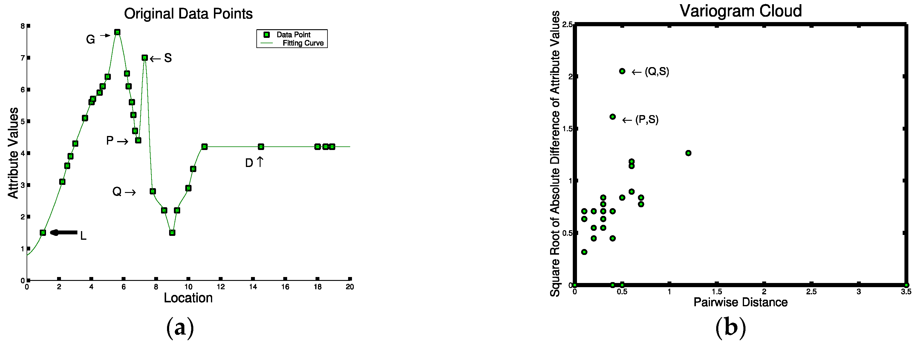

Table 1.
Approaches for addressing challenges of statistical significance testing of teleconnection patterns.
Table 1.
Approaches for addressing challenges of statistical significance testing of teleconnection patterns.
| Challenge | Approach |
|---|---|
| Spatial and temporal autocorrelation. | Spatio-temporal dependencies are captured by using a time series decomposition that requires each end of the dipole to share the same global component and using an auto-regressive term to capture time dependencies. |
| Seasonality and trends. | The time-series decomposition captures the seasonality and trends by extracting the underlying governing time series against local noise variations. |
| Generating random samples under the null hypothesis. | A “wild bootstrap” approach generates samples by multiplying random noise to the residuals |
© 2017 by the authors. Licensee MDPI, Basel, Switzerland. This article is an open access article distributed under the terms and conditions of the Creative Commons Attribution (CC BY) license (http://creativecommons.org/licenses/by/4.0/).
Share and Cite
MDPI and ACS Style
Xie, Y.; Eftelioglu, E.; Ali, R.Y.; Tang, X.; Li, Y.; Doshi, R.; Shekhar, S. Transdisciplinary Foundations of Geospatial Data Science. ISPRS Int. J. Geo-Inf. 2017, 6, 395. https://doi.org/10.3390/ijgi6120395
AMA Style
Xie Y, Eftelioglu E, Ali RY, Tang X, Li Y, Doshi R, Shekhar S. Transdisciplinary Foundations of Geospatial Data Science. ISPRS International Journal of Geo-Information. 2017; 6(12):395. https://doi.org/10.3390/ijgi6120395
Chicago/Turabian StyleXie, Yiqun, Emre Eftelioglu, Reem Y. Ali, Xun Tang, Yan Li, Ruhi Doshi, and Shashi Shekhar. 2017. "Transdisciplinary Foundations of Geospatial Data Science" ISPRS International Journal of Geo-Information 6, no. 12: 395. https://doi.org/10.3390/ijgi6120395
Note that from the first issue of 2016, this journal uses article numbers instead of page numbers. See further details here.