Article

Geovisualization for Association Rule Mining in Oil and Gas Well Data

1
Department of Geomatics Engineering, University of Calgary, Calgary, AB T2N 1N4, Canada
2
School of Information and Technology, Northwest University, Xi’an 710069, China
*
Author to whom correspondence should be addressed.
ISPRS Int. J. Geo-Inf. 2017, 6(2), 48; https://doi.org/10.3390/ijgi6020048
Submission received: 7 November 2016 / Revised: 21 December 2016 / Accepted: 13 February 2017 / Published: 18 February 2017

Abstract

:
Association rule mining on oil and gas data has recently been successfully used to help understand reservoirs; therefore, the visualization and understanding of the discovered association rules based on well locations and subsequent predictions based on the applicable areas of the rules are important. In this paper, two visualization methods—point- and surface-based geovisualization—are proposed for association rules from oil and gas well data. The point-based method represents association rules based on well locations, and the surface-based method represents potentially applicable areas through spatial interpolation and visualization. A case study has been carried out on a real cold production oil well dataset in western Alberta, Canada, and, the results illustrate the feasibility of the proposed geovisualization methods.

1. Introduction

Recently various data mining methods have been successfully utilized to help understand the reservoirs and enhance oil recovery [1,2,3,4]. Association rule mining is one of the most popular data mining methods and was first proposed for extracting interesting correlations, frequent patterns, associations or casual structures among the item sets from transaction data or other data repositories [5]. Association rule mining in oil and gas well data is a very promising approach for understanding and improving oil recovery.
Oil and gas well data generally includes well locations and other non-spatial attributes, such as reservoir property parameters (e.g., pore volume, porosity, permeability) and production performance parameters (e.g., peak value and effective yield) [3]. After the values of the non-spatial parameters are transformed into a set of sub-ranges, association rule mining algorithms such as Apriori [6] can be applied to the discretized data. The quantitative relationships between reservoir properties influencing oil recovery and oil production performance can then be discovered [3]. However, there are still some challenges in the understanding and identification of the interesting association rules from oil and gas well data.
The association rules discovered from non-spatial oil and gas well data only include the patterns between reservoir properties and oil production performance. However, oil and gas well data also has geospatial attributes, i.e., well locations. The interestingness of the rules does not depend only on the included patterns, but also relies on the locations and distributions of the wells that the rules match. Therefore, the rules need to be associated with the locations of the wells. However, the existing visualization methods for association rules fall short: most methods, such as scatter plots, matrix visualizations, graphs, mosaic plots and parallel coordinate plots [7,8,9,10,11,12,13], have been designed to help identify interesting association rules discovered from non-spatial datasets and, thus, focus more on the visualization of the rule content characteristics.
Geovisualization generally refers to a list of tools and techniques supporting geospatial data analysis, integrating cartography, geographic information system (GIS) and scientific visualization [14]. Geovisualization does not merely include representation of the source or raw geospatial dataset through an accessible and interactive interface (e.g., a map) by simple display techniques (e.g., symbols, colors), but also assists users in learning new geospatial trends and patterns hidden behind the dataset. Therefore, geovisualization can help associate the spatial information of wells with the interesting rules in oil and gas well data.
In addition to relating the well locations with the association rules, the building and visualization of an association rule with respect to applicable areas is also worthy of research. The applicable areas of the rules, i.e., the continuous surfaces where the rule may be relevant, are also very valuable for reservoir engineers. However, the continuous surfaces cannot be directly constructed, since the well locations are an irregular array of discrete points. The geovisualization of the association rules in oil and gas well data needs to be combined with proper spatialization techniques that can fill in data between the wells.
Spatial interpolation is the process of using points with known values to estimate values at other points [15]. Through spatial interpolation, the value of a certain attribute at a location with no recorded value can be estimated using the corresponding known value of the attribute of nearby sample wells. If the spatial dependence appears in the attributes of the well data, spatial interpolation can be an appropriate spatialization technique.
In this paper, two geovisualization methods—point-based and surface-based—are proposed for association rules in oil and gas well data, in order to better understand wells. The contributions of the paper are summarized as follows:
The point-based geovisualization method links association rules with well locations. The method uses different symbols to highlight the well locations that satisfy the rules. Reservoir engineers can better understand the rules and find possible distribution patterns of the wells by the visualized oil well locations on the map.
Another visualization method, surface-based geovisualization, builds and represents the areas on the map for an interesting rule where the rule may be applicable. The method is based on spatial interpolation and map layer overlapping. The surface-based geovisualization can assist users in making decisions or predictions based on the patterns included by the discovered interesting rules.
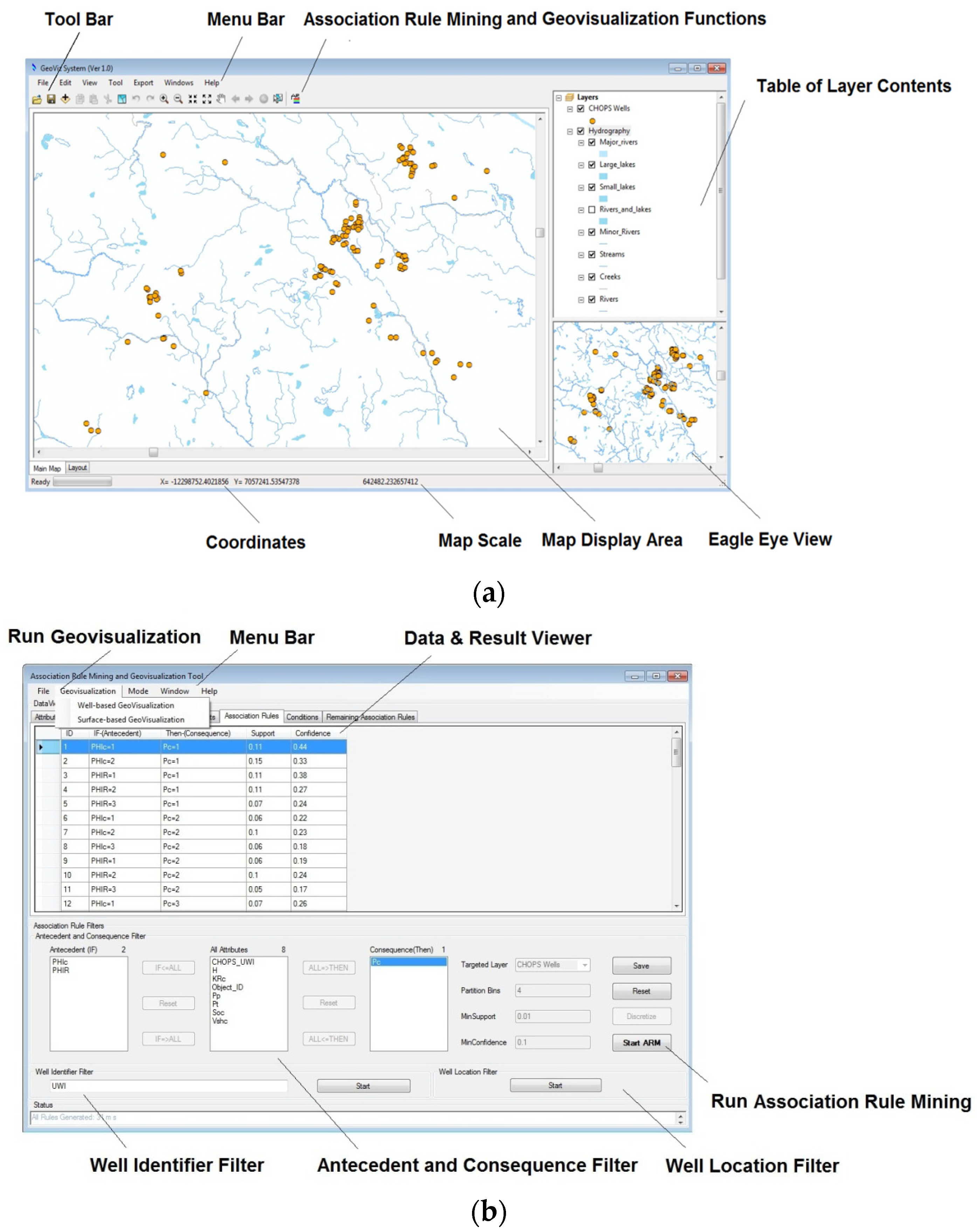
A system prototype for in Oil and Gas Well Data, called Association Rule Mining and Geovisualization (ARM-GEOVIZ) System, is developed for association rule mining and visualization of found rules in oil and gas data. The system prototype integrates association rule mining with the proposed point-based and surface-based visualization methods.
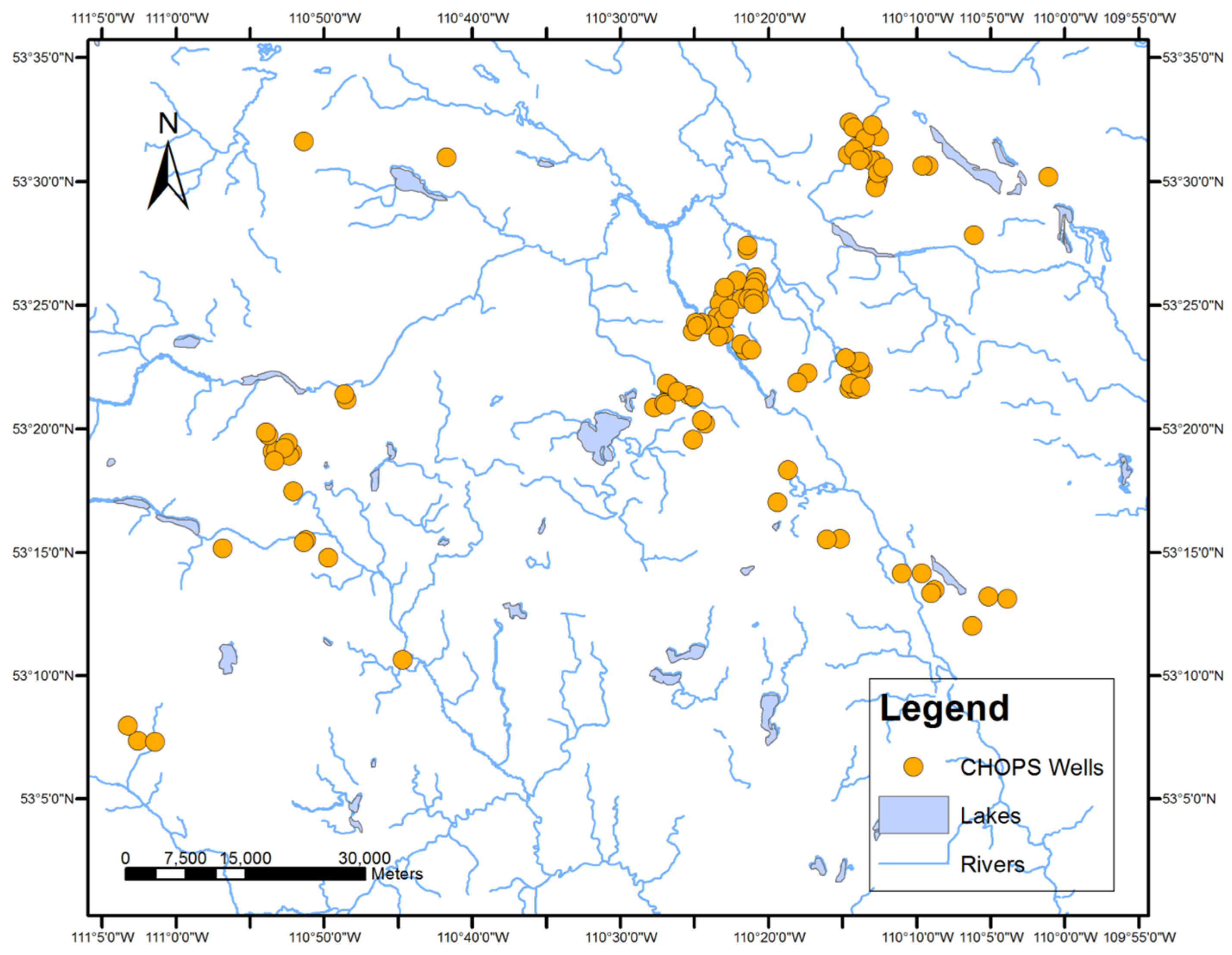
A case study was conducted on a real cold production oil well dataset for the Lloydminster heavy oil block in Alberta, Canada. The case study validated the feasibility of the two new geovisualization methods for association rules.
The rest of this paper is organized as follows: Section 2 reviews association rule mining, existing visualization techniques for association rules in non-spatial data, and common spatial interpolation techniques. Section 3 introduces the detailed methodology of the proposed geovisualization techniques for association rules in oil and gas well data. The two geovisualization methods and the ARM-GEOVIZ system prototype are illustrated through a case study with real oil well dataset in Section 4. Section 5 presents the conclusion.

2. Related Work

Association rule mining, visualization techniques for association rules and several spatial interpolation techniques are briefly reviewed in the following subsections.

2.1. Association Rule Mining

Association rule mining was first introduced to analyze transaction data and derive association rules [5]. In the definition of the association rule, let D be the set of all items and X and Y be two subsets of D. An association rule with respect to X and Y can be in the form of (or IF { X } THEN { Y }), where, X , Y D , X Y , and X , Y . X is called the antecedent and Y is the consequence.
The concepts of support and confidence are essential in defining the interestingness of an association rule. The support of rule is defined as the percentage of transactions that consist of X and Y to the total number of transactions, i.e., ( X Y ) = P ( X Y ) . The confidence of rule X Y is the percentage of transactions that consist of X and Y to the number of transactions that only contain X. The definition is in the form of conditional probability confidence ( X Y ) = P ( Y   |   X ) = P ( X Y ) / P ( X ) . Traditionally, the rules that are satisfied with large support and confidence values are considered to be strong or interesting.
Apriori is the most well-known algorithm for association rule mining over transactional databases [6]. It proceeds by identifying the frequent individual items in the database, and then groups of frequent item set candidates are generated and tested against the data. The algorithm terminates when no further frequent item sets are found. The frequent item sets determined by Apriori can be used to determine association rules.

2.2. Traditional Visualization Methods for Association Rules

Several visualization techniques for association rule mining in transaction data or other non-spatial datasets have been recently proposed in order to help users analyze discovered association rules.
Scatter plots visualize association rules as scatter points on two-dimensional or higher coordinate systems. In a two-key plot, the coordinate axes x and y represent the support and confidence values of the rules, and the color of the scatter points represents the total numbers of the antecedent and consequent items within the rules [7].
In a parallel coordinate plot, association rules are represented as polygonal lines on a coordinate system with shared x and y axes [8]. The antecedent and consequence items of the rules are used for one coordinate axis, and the other axis is used to represent the corresponding positions of antecedent and consequence items in rules.
Graph-based plots represent association rules as figures with vertices and edges [9,10,11,12]. The vertices are used for the antecedent and consequence items of the rules. The relationship of the items of one association rule is shown by the connected edges of the items.
The visualization methods can help find the content characteristics hidden behind the association rules. For example, scatter plots can display the distribution of interesting measurements of multiple rules. Parallel coordinate plots are suitable to represent the compositions of the antecedent and consequence items of the rules. The relationships among the rules in terms of certain items can be found by using graph-based plots. However, these methods have been mainly proposed for rules from transactional datasets and do not take spatial attributes into account.

2.3. Geovisualization

On the basis of scientific visualization, geovisualization integrates GIS and cartography to communicate geospatial information in support of geospatial analysis [14]. The geospatial data can be displayed by a map interface, and unexpected geospatial trends and patterns hidden behind the data can be discovered.
Geovisualization has recently become widely used in many scientific disciplines. Aoidh et al. proposed a geovisualization method where symbology was explored for communicating the landscape genetic information in an intuitive way [16]. Gienko and Terry introduced a geovisualization method for representing and predicting cyclone behaviour, where several spatial interpolation techniques were successfully combined with geovisualization for identification and analysis of cyclone features [17]. The above methods are based on symbology and spatialization techniques, but are not aimed at visualization of the association rules from geospatial data.

2.4. Spatial Interpolation

Under the assumption that the estimated value of an interpolation point should be influenced more by nearby control points than distant control points, spatial interpolation can fill in data between sample points. Spatial interpolation methods can be categorized into stochastic and deterministic methods.
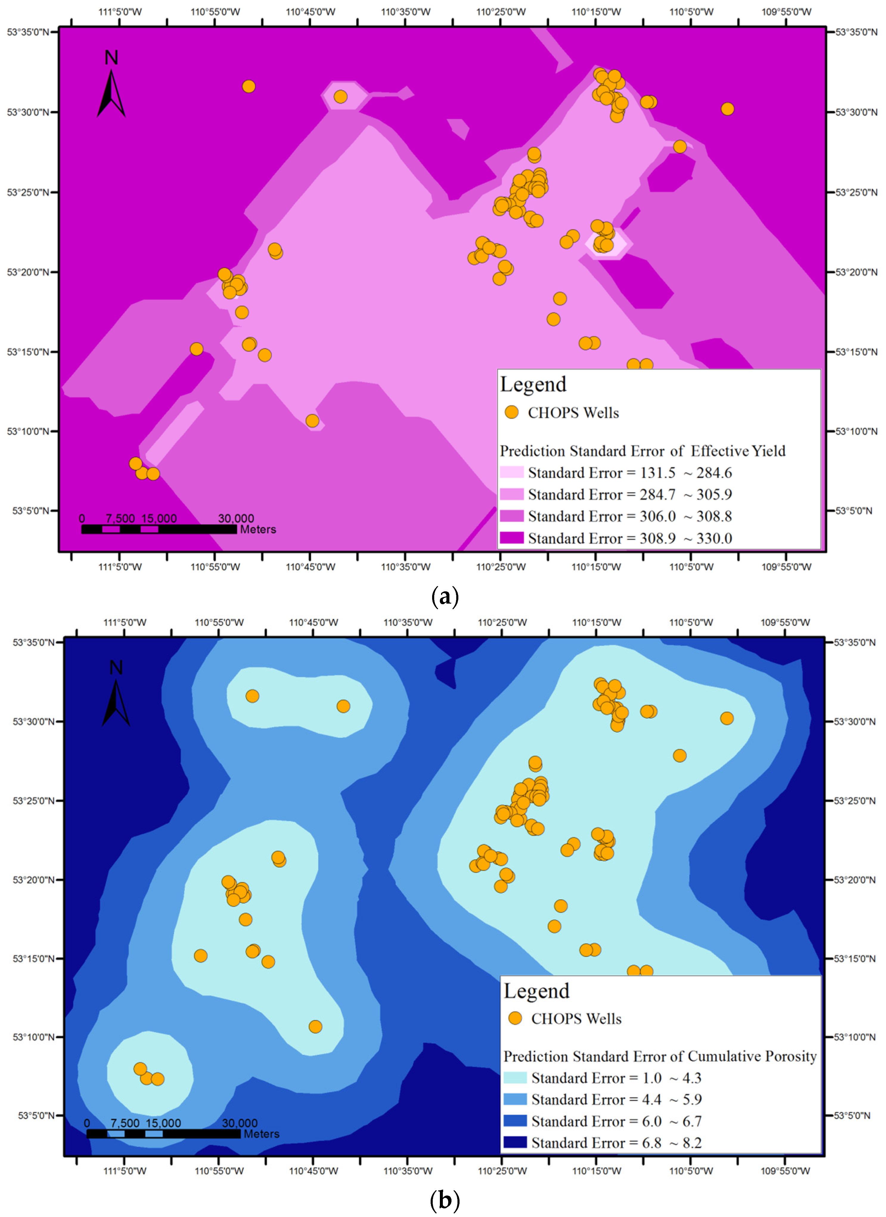
A stochastic interpolation method provides assessment of prediction errors by estimated variances in the form of prediction standard errors with interpolated values. Kriging interpolation is one of most common spatial stochastic interpolation methods. It cannot only interpolate the value of a certain attribute for an unknown (interpolation) point with the known attribute values of its neighbour points, but can also offer prediction errors with estimated values to assess the quality of the interpolation. Kriging assumes that the spatial variation of an attribute to be interpolated may be composed of a spatially correlated component representing the variation of the regionalized variable, a drift representing a trend, and a random error component.
A deterministic interpolation method does not involve probability theory, thereby offering no assessment of errors with predicted values. Spline interpolation estimates values using a mathematical function that minimizes overall surface curvature, ending up with a smoother statistical surface. The surface passes exactly through the control points. In Inverse Distance Weighted (IDW) interpolation, a weight is assigned to each neighbourhood point within a predefined radius for an interpolation point. The weight decreases as the distance from the interpolation point to its neighbourhood points increases. The estimated value of the interpolation point is the weighted average of its neighbourhood points. Trend surface interpolation approximates the unknown values of interpolation points with a polynomial equation. The order of the polynomial equation can be adjusted according to the complexity of the specific situation.
Given the different characteristics of deterministic and stochastic interpolations, their applicability to oil and gas well data is explored by using real well data in the following sections.

3. Methodology

3.1. Association Rule Mining on Oil and Gas Well Data

Each well record in the oil and gas dataset contained reservoir properties and oil and gas production performance properties of the well. Moreover, the location of each well was denoted in longitude and latitude coordinates.
The processing of the association rule mining includes the following steps. First of all, the continuous values of the reservoir property and oil production performance parameters in the source oil and gas well data were first discretized. For example, a numeric value (73.2) of the reservoir property attribute cumulative pore volume could be transformed into discretized value “1”, which represented a range of values from 59.2 to 94.4. The discretization process could be accomplished through k-means clustering method. K-mean clustering algorithm is an effective and efficient clustering algorithm. It first partitions the data into k nonempty subsets, and then calculates seed points as the centroids of the clusters of the current partition (i.e., mean point of the cluster). Next, it assigns each data object to the cluster with the nearest seed point. The process continues until no more new assignment. The parameter of k-mean clustering method is the value of k, which must be fixed before the computation.
Next, the association rule mining algorithm such as Apriori [6] discussed in Section 2.1 could then be applied to the processed data. The main objective in applying association rule mining is to discover interesting relationships between reservoir properties and oil production performance. Each discovered rules is in the form of:
IF {Reservoir properties hold certain conditions} THEN {Production Performance is within certain range}; [Support = n%; Confidence = m%] where the IF part is called the antecedent; the THEN part is called the consequence; support n% denotes that n% wells in the whole dataset satisfy this rule; confidence m% denotes that, among all wells that satisfy the reservoir property conditions in the antecedent, m% of these wells also satisfy the consequence. Support and confidence are two important measurements for rule interestingness.
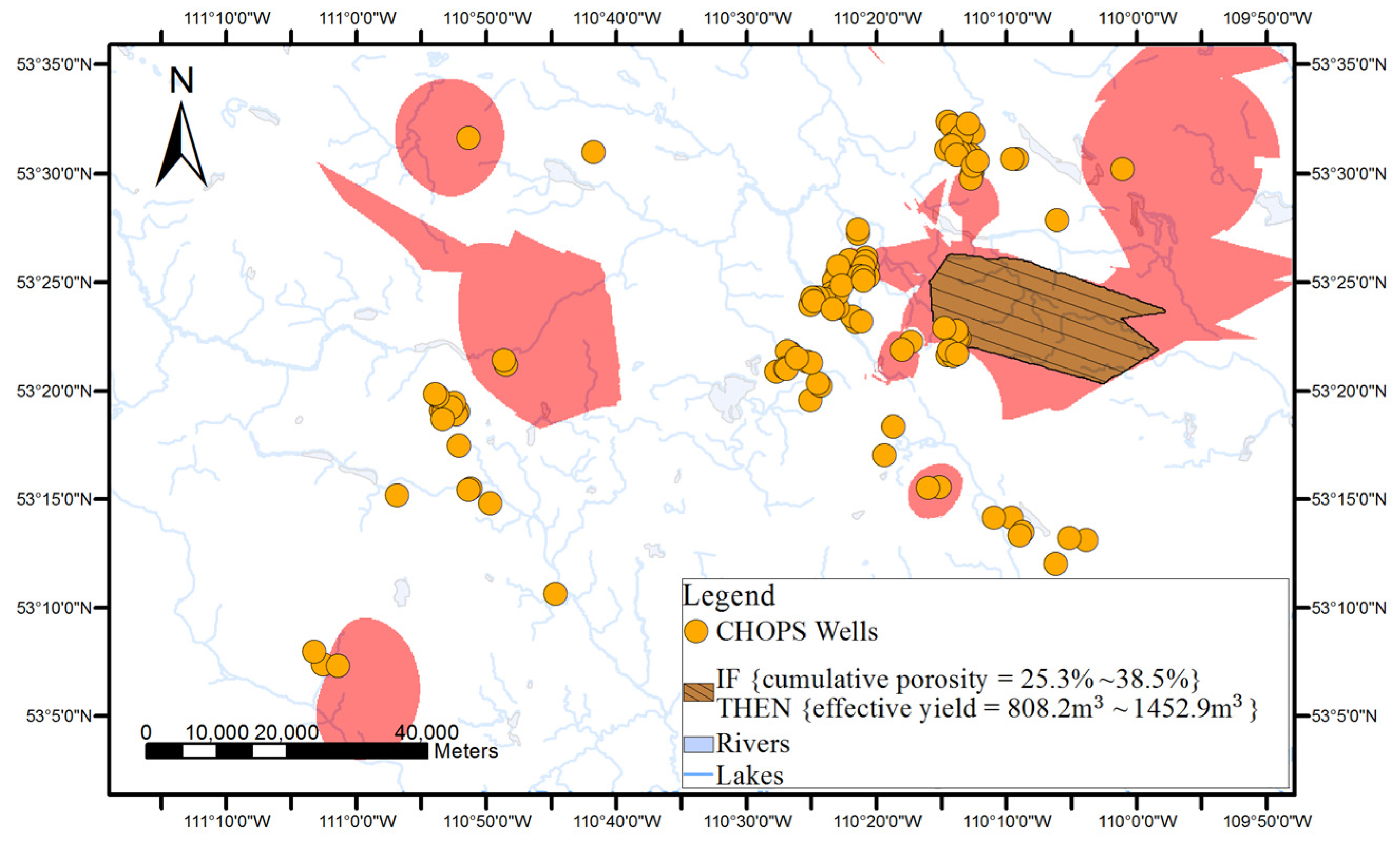
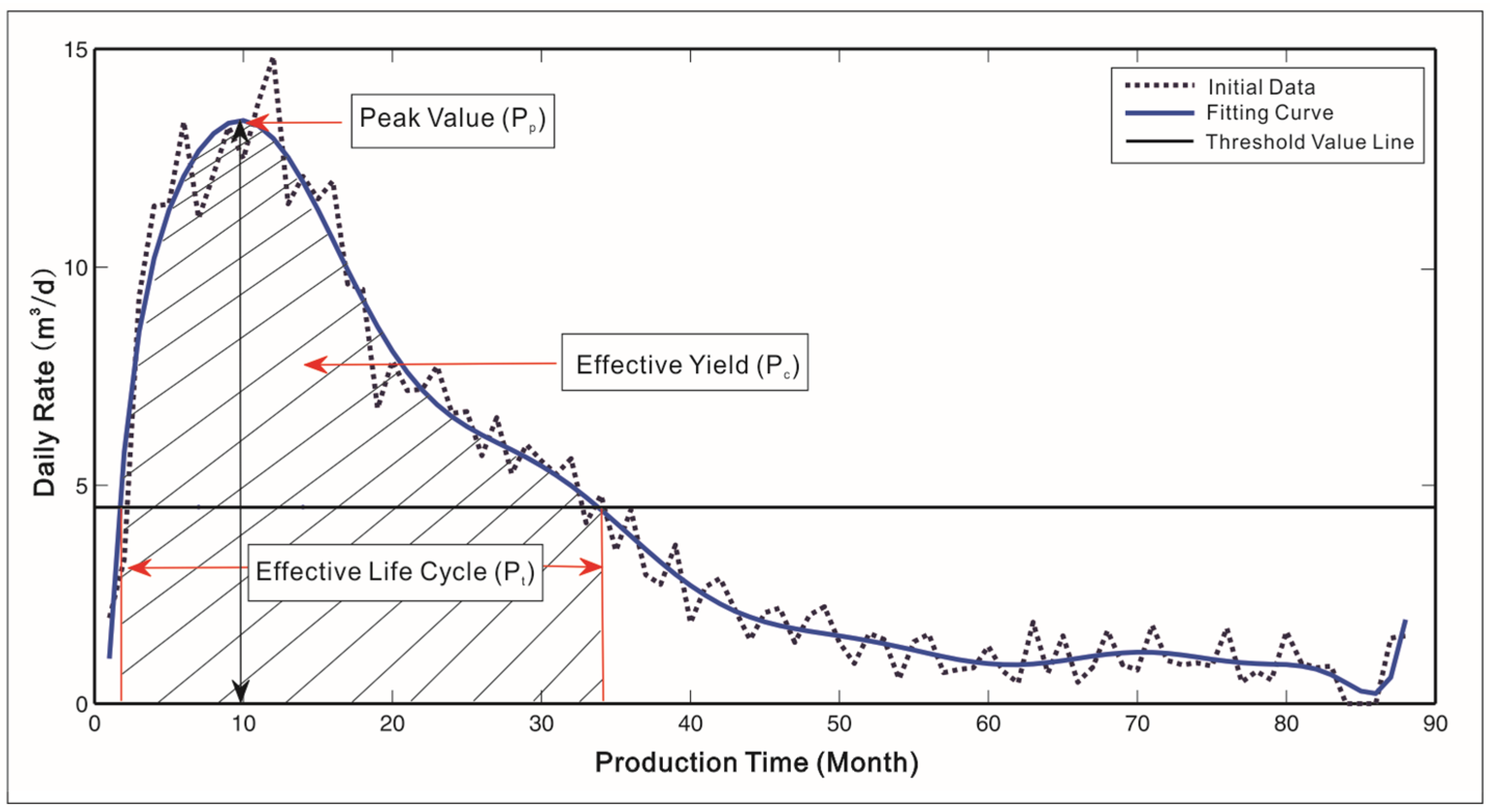
An example of the discovered association rules is IF {cumulative pore volume = 168.8–291.2} THEN {effective yield = 808.2–1452.9 m3}, [support = 15%, confidence = 80%] i.e., if the reservoir property’s cumulative pore volume is between 168.8 and 291.2, then the effective yield is in the range between 808.2 m3 and 1452.9 m3. The rule was supported by 15% of the data in the dataset and among wells with the cumulative pore volume between 168.8 and 291.2, 80% of the wells has the effective yield between 808.2 m3 and 1452.9 m3.

3.2. Geovisualization for Association Rules

Mining association rules in oil and gas well data usually generate a large number of association rules. Setting minimum thresholds for traditional interestingness measurements, such as support and confidence, may help find interesting rules; however, some potentially interesting rules with relatively low interestingness measurements may be missed. For an association rule found in well data, the interestingness of the rule depends not only on its support and the confidence, but also on the locations and distributions of the wells that match the rule. However, there are challenges to determining the interesting rules and to better understanding the discovered rules. Moreover, the potential applicable areas of the interesting rules are critical to reservoir engineers, who make predictions on oil production based on reservoir properties determined with the interesting rules.
In this paper, point- and surface-based geovisualization methods are proposed for the visualization of the association rules in oil and gas well data and are described in the following subsections. Point-based geovisualization conceptualizes an association rule with regards to well locations, and surface-based geovisualization builds the applicable areas for an association rule based on spatial interpolation techniques and then effectively represents the areas on a map.

3.2.1. Point-Based Geovisualization

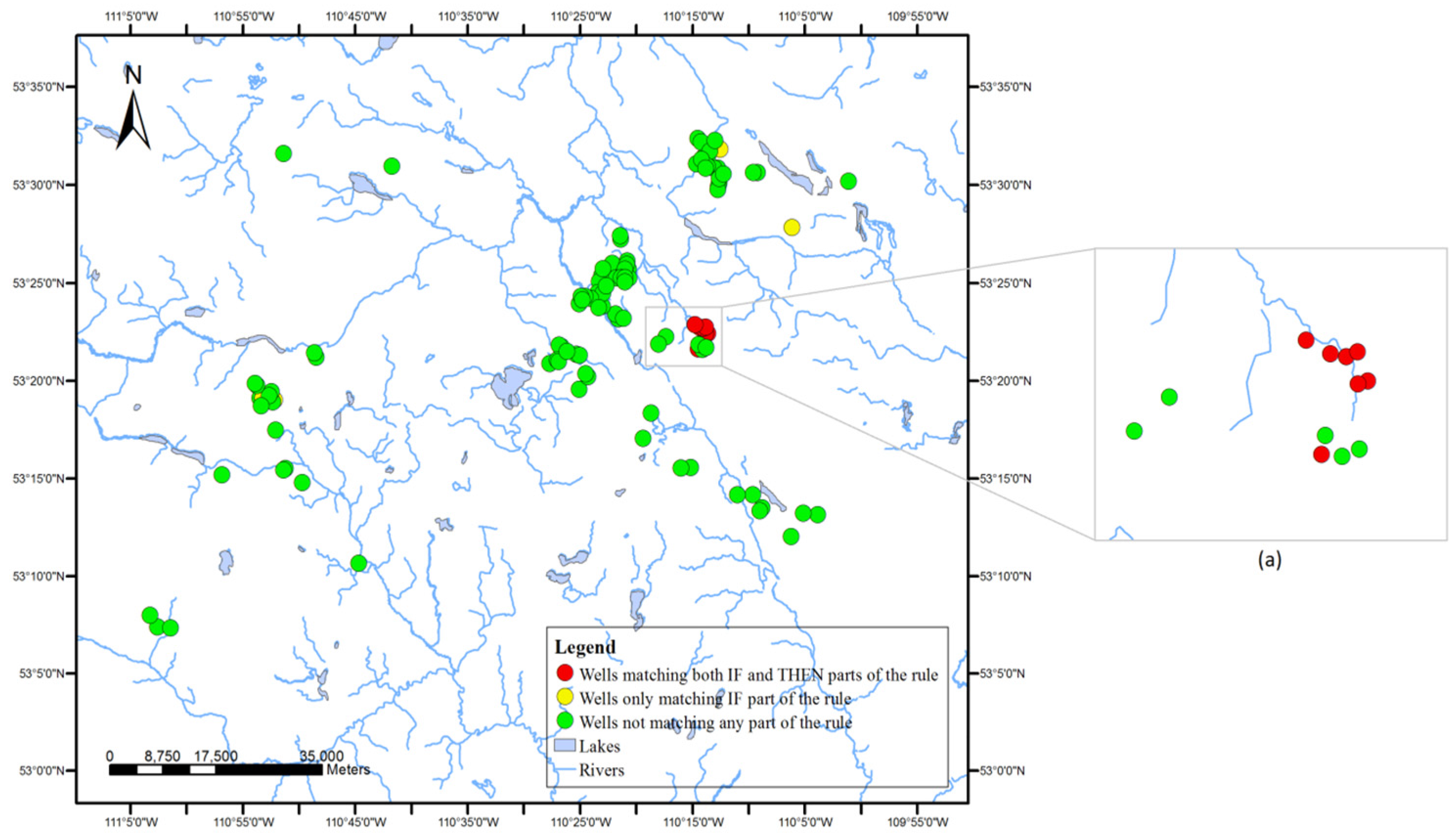
Point-based geovisualization uses different symbols to show the locations (points) of wells, depending on their relationship with association rules in well data. The geospatial distribution of the wells associated with one association rule was visualized on a map with the following steps. First, all wells were categorized into three groups according to the extent of satisfaction of the rule.
Group 1: wells with the same ranges of reservoir properties and production performances described in the rule (i.e., satisfied both antecedents and consequences of the rules).
Group 2: wells with the same range of reservoir properties described in the rule, but a different range of production performance (i.e., satisfied the antecedents but not the consequences of the rule).
Group 3: wells with different reservoir properties and production performances than described in the rule (i.e., neither satisfied the rule).
The above categorization scheme can reflect the two traditional interestingness measurements (support and confidence) on the map. For the association rules in well data, the support is the percentage of the wells in the whole dataset satisfy this rule; and, the confidence is the percentage of the wells among all wells that satisfy the reservoir property conditions in the antecedent. Specifically, by comparing the wells that satisfy the association rule (Group 1) and those that do not (Group 3), support of the rule can be understood; and, the wells that support the rule can be located on the map. Similarly, the confidence of the rule and the locations of the wells giving the confidence of the rule can be identified by comparing the wells satisfying the rule (Group 1) and those only satisfying the antecedents and not the consequences of the rule (Group 2).
After categorization, the well locations of the three different groups were represented on a map using different symbols. Point-based visualization connects the discovered rules with the well locations. Users (i.e., reservoir engineers) can easily identify the wells satisfying the rule and can reversely find rules associated with the well. The comparison and analysis of the geospatial distributions of the three groups of categorized wells on the map can also help users in learning about the support and confidence of each discovered rule.

3.2.2. Surface-Based Geovisualization

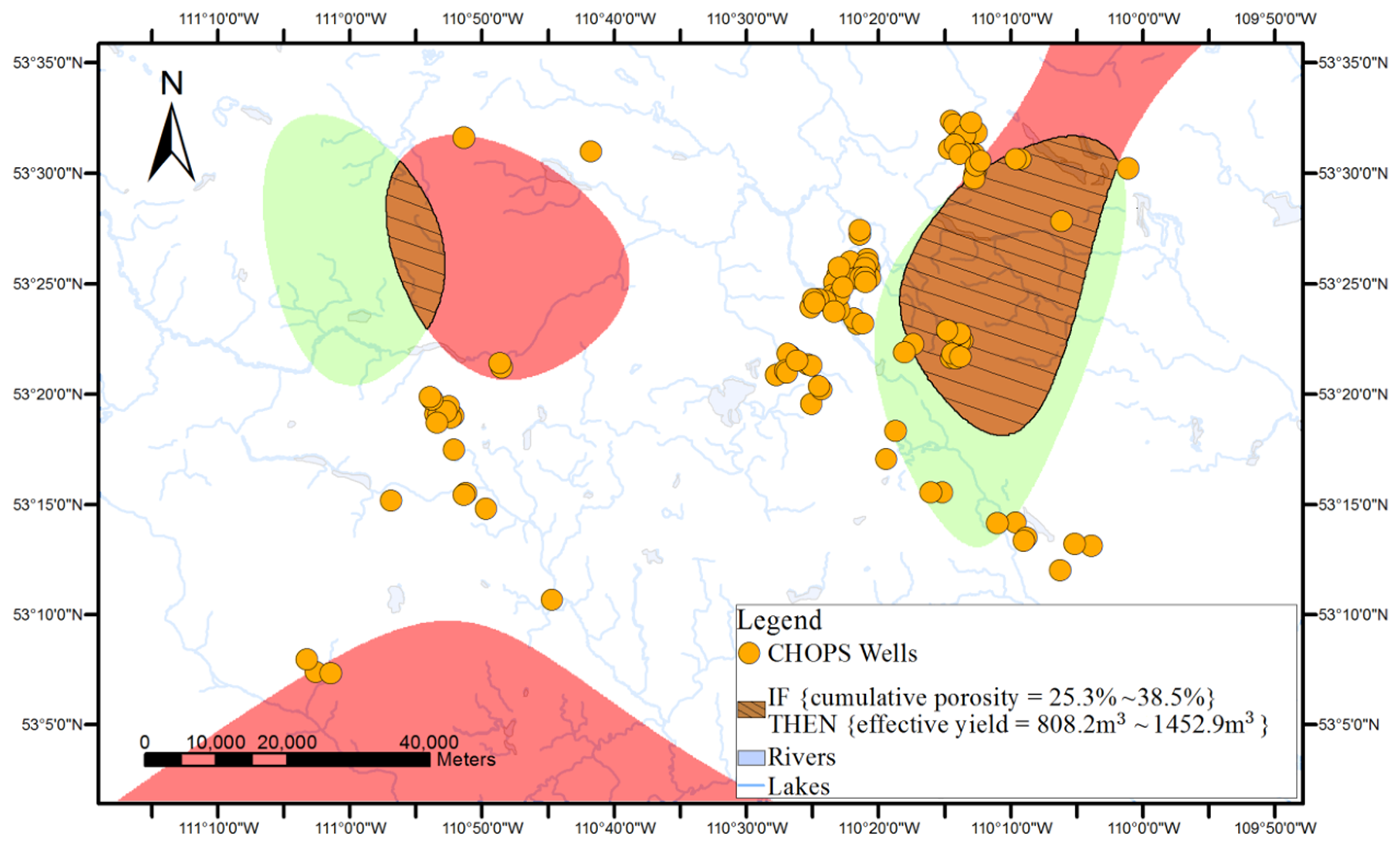
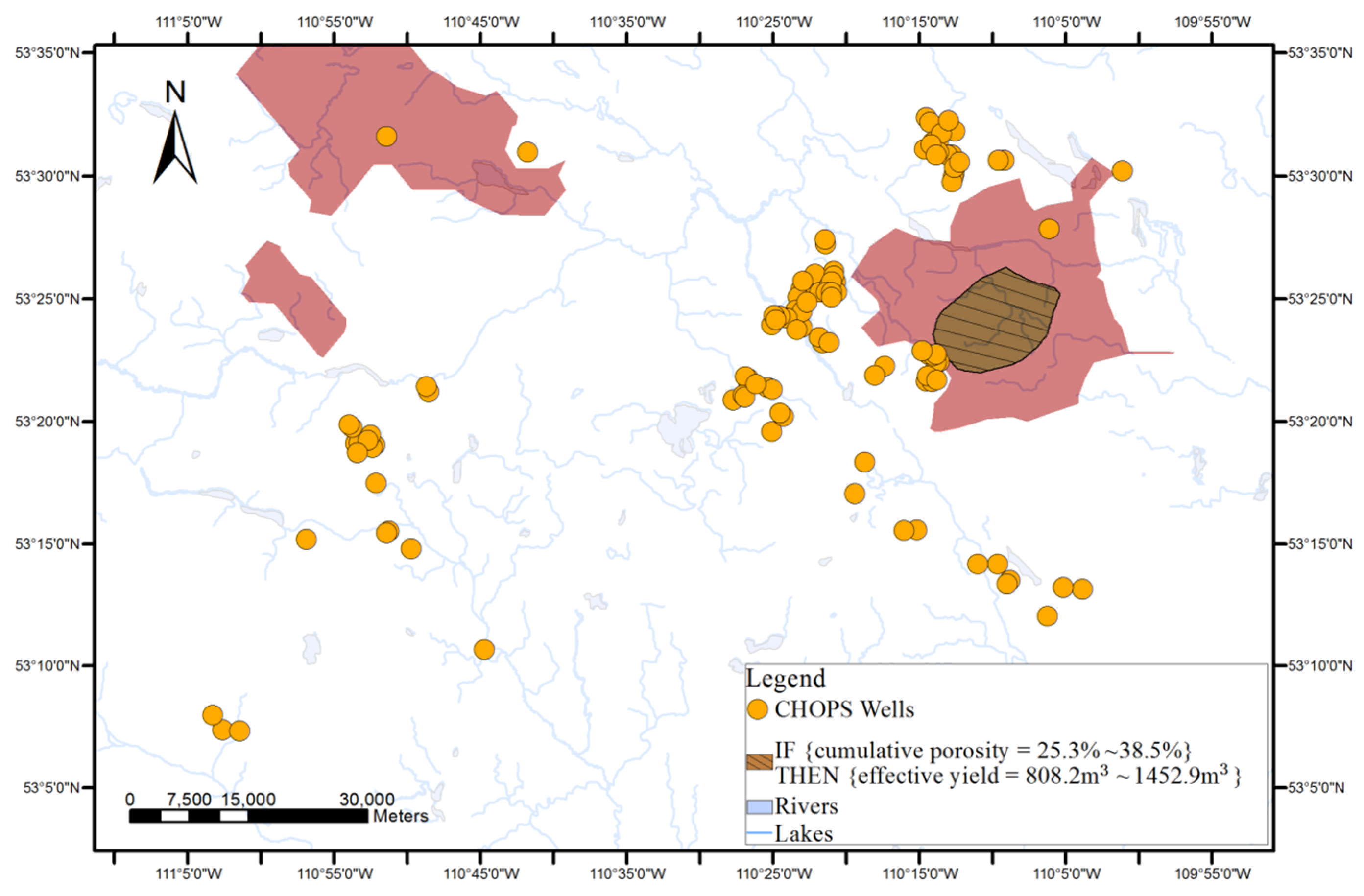
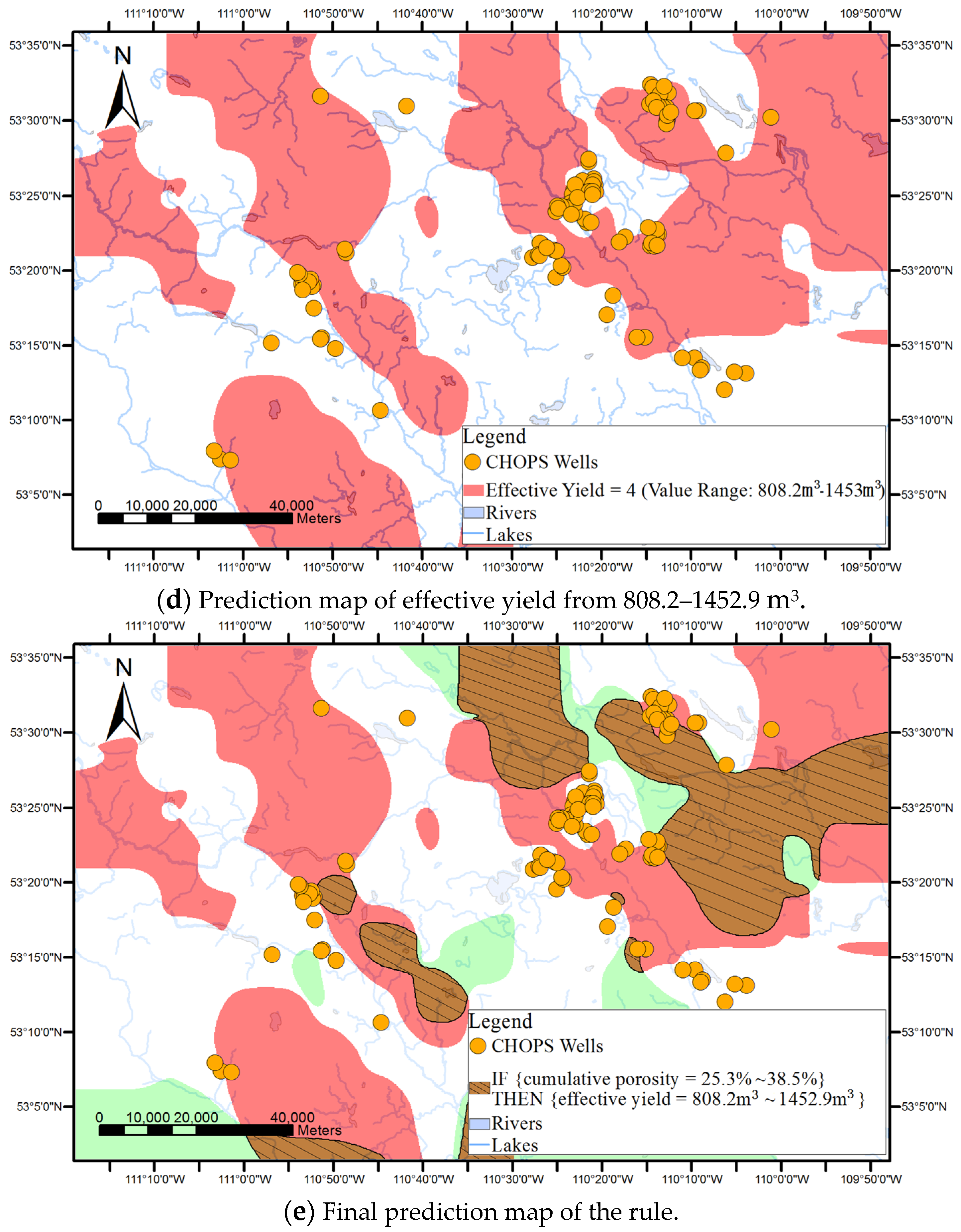
Surface-based geovisualization extends the conceptualization of the rule from discrete points to continuous surfaces, with the aim of generating and representing areas where the rule may be applicable.
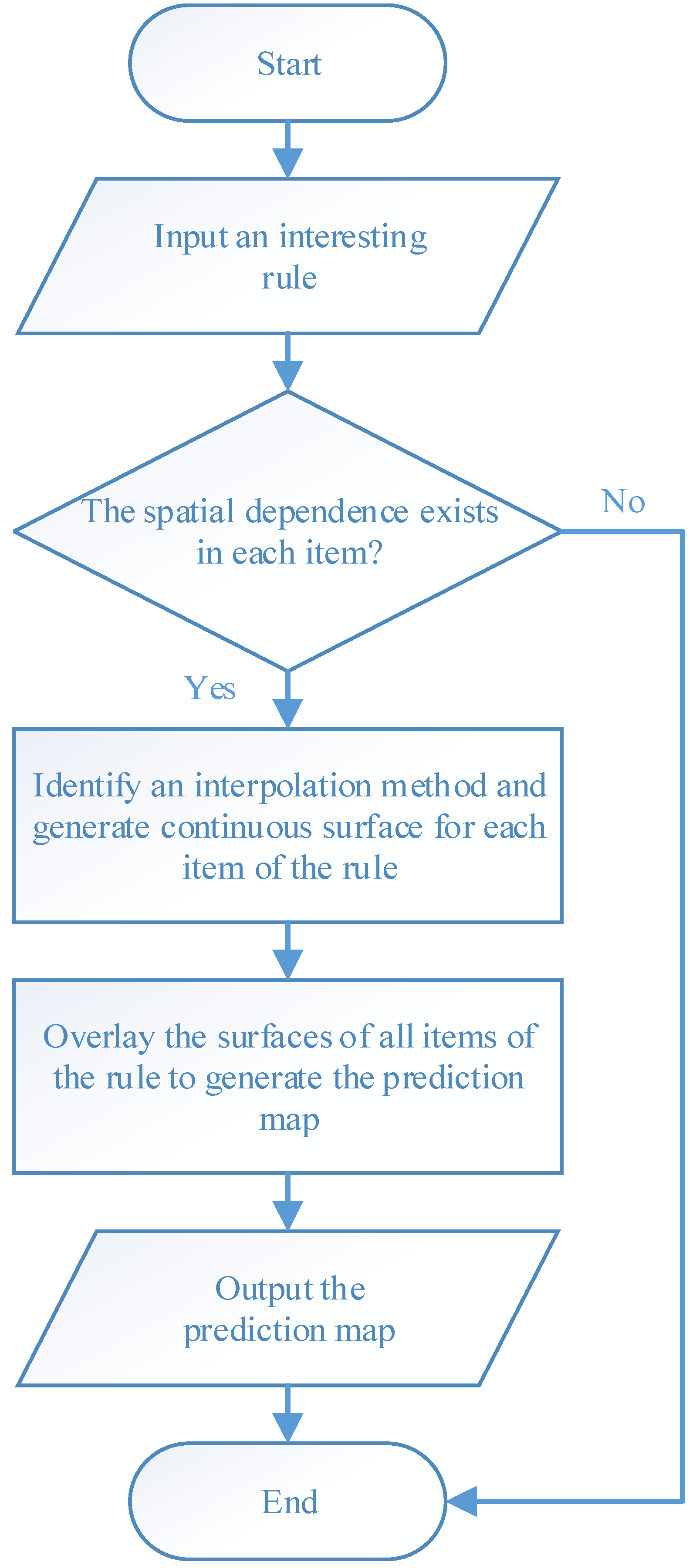
As shown in Figure 1, surface-based geovisualization of an association rule mainly includes the following steps. First, the spatial dependence of all the attributes appearing in the antecedents and consequences of the rule are examined. If the spatial dependence does not exist in the attributes, the surface-based geovisualization method is not applicable for the rule. Otherwise, continuous surfaces of the attributes are generated by applying a deterministic or stochastic spatial interpolation method on the well data. Next, the corresponding application areas of antecedents and consequences of the rule are extracted from the continuous surfaces and indicated by different colours. Finally, a prediction map of the rule is obtained by overlaying the application areas of the antecedents and consequences of the rule.
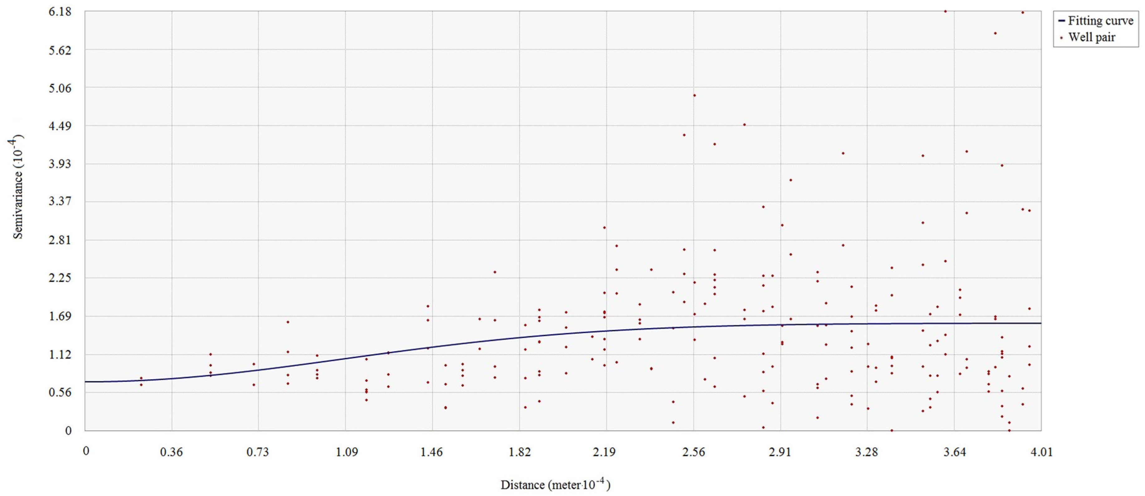
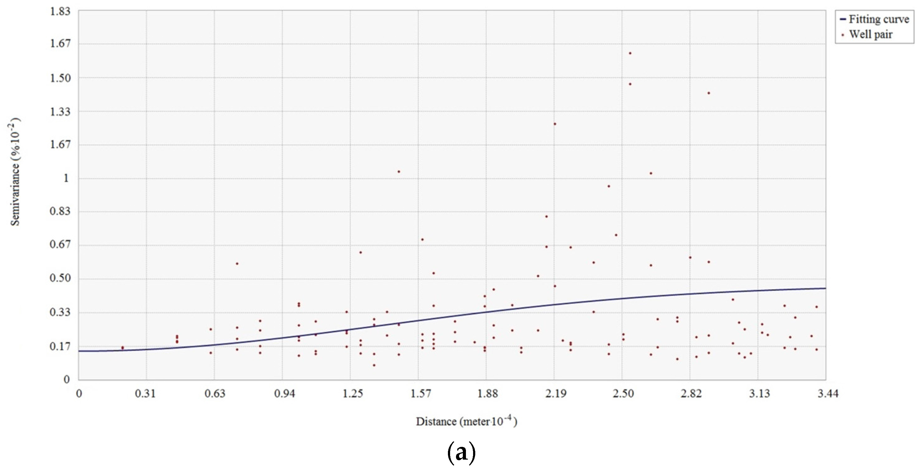
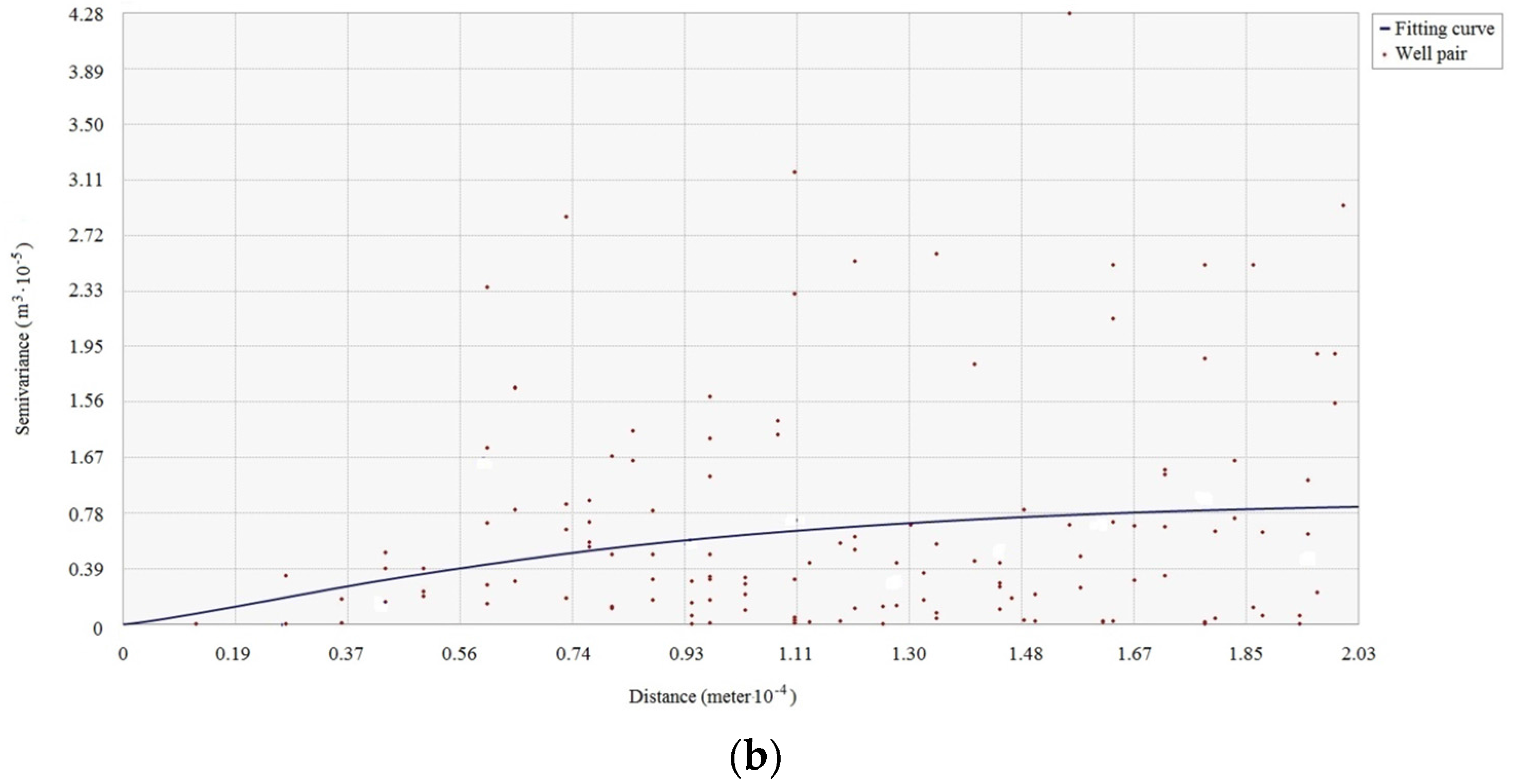
The existence of spatial dependence in the attributes in the studied area is the precondition for the use of spatial interpolation. The spatial dependence of each antecedent or consequence attribute of the association rule should be examined before using spatial interpolation. The spatial dependence of attributes can be checked by semi-variogram clouds. If spatial dependence of a reservoir property attribute exists in the studied reservoir area, the semi-variance decreases with increasing spatial distance in the semi-variogram cloud of the attribute.
Figure 2 shows a semi-variogram cloud of the cumulative pore volume attribute in an area. Since the semi-variance increases as the spatial distance increases in the cloud, the semi-variogram cloud suggests that spatial dependence appears in the cumulative pore volume to some degree. Pairs of sample wells that are closer in distance on X-axis have more similar semi-variance values (Y-axis) for the cumulative pore volume than well pairs that are farther apart.
Note that directional influences also need to be considered when generating semi-variogram clouds. The spatial dependence of an attribute can be stronger in specific directions. The directional influences may come from geological structures or a variety of other more complex processes. The directional influence of spatial dependence needs to be incorporated into the spatial dependence validation of each antecedent or consequence attribute of the association rule.
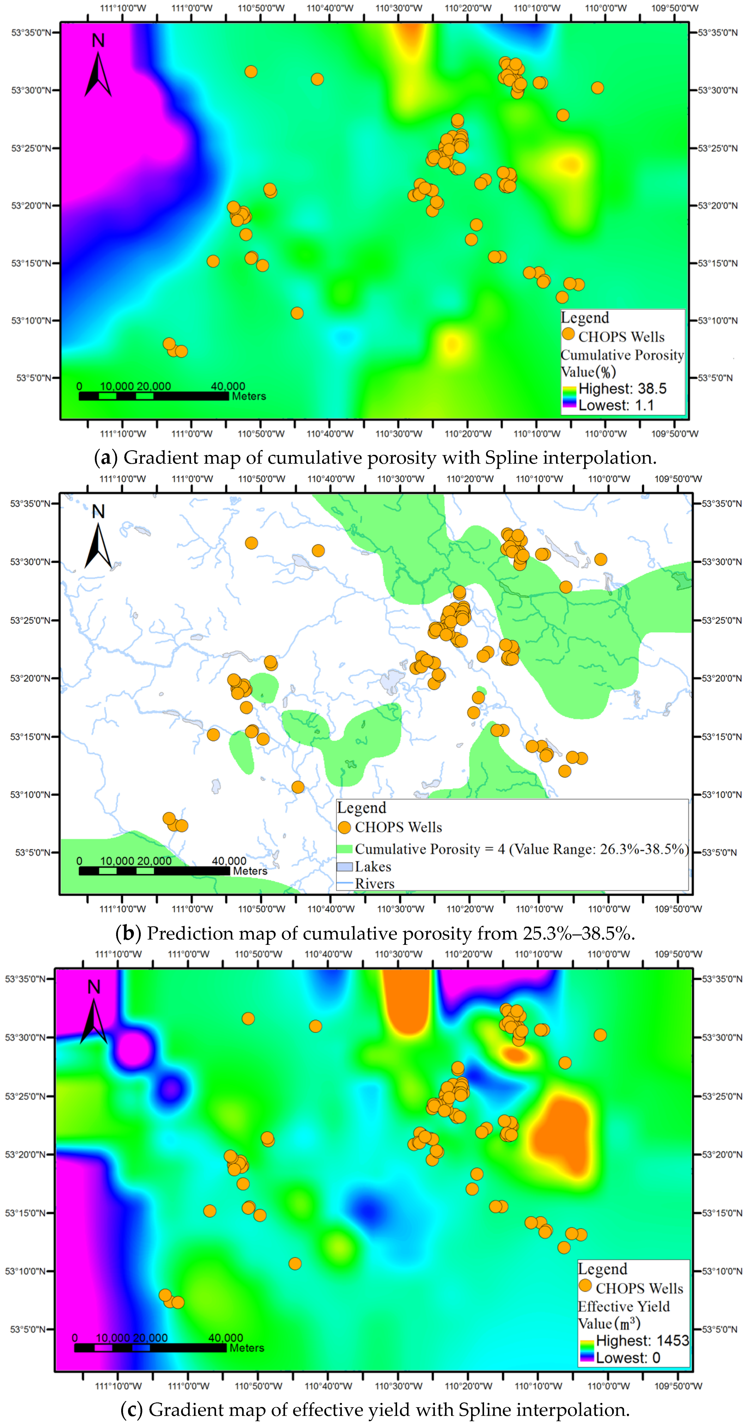
If spatial dependence of the antecedent and consequence attributes of the rule exists in the studied area, deterministic or stochastic interpolation methods are used to generate continuous surfaces for the attributes. Wells are represented as the point features discretely distributed on the map. Spatial interpolation then fills in the missing data between the wells based on the attribute values of the wells, i.e., the value of the attribute at a location with no recorded data can be estimated using the corresponding known value of the attribute of nearby sample wells.
In terms of the format of the geospatial data, the spatial interpolation generates a raster layer with estimates made for all cells for each antecedent or consequence attribute of an association rule from a vector layer containing oil wells, where the value of each attribute is known. After this step, each attribute appearing in the association rule to be visualized will have an interpolated continuous surface.
The applicable areas of the antecedents and consequences of the rule are then extracted and rendered from the surface of each attribute. For instance, the applicable areas of an antecedent of an association rule (e.g., cumulative pore volume = 59.2%–94.4%) can be gained by extracting the cells whose interpolated values belong to the range from 59.2% to 94.4% from the interpolated continuous surfaces of the cumulative pore volume.
Finally, a prediction map of the applicable areas of the rule is obtained by overlaying all interpolated continuous surfaces of the attributes appearing in the rule.

4. ARM-GEOVIZ System Prototype and a Case Study

4.1. ARM-GEOVIZ System Prototype

Based on the proposed geovisualization methods, we developed a system prototype, called ARM-GEOVIZ. The GUIs of association rule mining and geovisualization were developed using C# programming language with integration of the ESRI ArcObjects API. The prototype supports diverse data formats (*.mxd map file, *.lyr layer file, *.shp shape file, *.mdb geodatabase file) and displays them on the map. The prototype mainly included four components as shown in Figure 3: A well database, association rule mining function, geovisualization function, and graphical user interface (GUI).
Well Database: The well database saved both the spatial and non-spatial data. The spatial data included the well locations (i.e., longitude and latitude) and spatial objects representing wells (i.e., points). The non-spatial data included the unique well identifier (UWI), reservoir properties and oil production data. The UWI was unique to each well and was used as the primary key in the database. The non-spatial data were connected with the spatial data using the primary key of UWI.
Association Rule Mining Function: The continuous values of the reservoir property and oil production performance parameters in the source data were firstly discretized by the data transformation sub-function. Compared with the classic equal width or frequency methods, both the self-organizing map and k-means techniques can discretize data by keeping the distribution similar to that of the attribute’s original one and can be more intuitive [18]. Therefore, in the system, both methods were implemented as the data transformation functions. Apriori algorithm then discovered the discovered association rules among the discretized attributes. The association rule filtering sub-function filter the interesting rules with user specified antecedent and consequence support and confidence values.
Geovisualization Function and Graphical User Interface (GUI): Figure 4a shows the main GUIs of ARM-GEOVIZ system prototype. The main interface consists of map display area, table of layer content, eagle eye window, menu and tool bar. The map display area in the middle of the interface shows the visualization of interesting rules with the designated map scale and coordinates. The layer table on the right of the interface shows the map layers. The eagle eye window shows a global view of the current map. The top of the interface contains the menu and tool bar where association rule mining and geovisualization functions can be accessed. Through the main interface, the user can execute the association rule mining and geovisualization by clicking the Association Rule Mining and Geovisualization Function button on the tool bar. Figure 4b shows the user interface of the association rule mining and geovisualization. From top to bottom, there are the Menu Bar, Data & Result Viewer, Association Rule Mining, Rule Filters, and Message Box. Geovisualization function including point- and surface-based methods can be launched under the Menu Bar. In the filters, users can screen out interesting rules from all of the resulting association rules generated and listed in the Data & Result Viewer, by setting or selecting the antecedents and the consequences, unique well identifiers, and well locations. Next, users can select point- or surface-based methods under Geovisualization and then click each individual interesting rule in the Data & Result Viewer to obtain the geovisualization results on the map in the main interface.

4.2. Case Study

A case study was carried out on real data of Cold Heavy Oil Production with Sand (CHOPS) well for the Lloydminster heavy oil block in Alberta, Canada.

4.2.1. Data Collection and Pre-processing

The Lloydminster heavy oil block is a large reservoir zone located in the central eastern part of the province of Alberta in Canada. In the block, more than 3000 wells have been drilled. One hundred and eighteen cold production oil wells were selected from the block based on the following selection criteria: (1) drilling date between 1992 and 2005; (2) vertical well; and, (3) one perforation formation. The distribution of the studied 118 CHOPS wells of the area is shown in Figure 5.
The source data of the 118 studied CHOPS wells in the case study were collected and saved in the database [19]. Each well record in the data contained reservoir property and oil production performance parameters of the well, and each well had its geospatial location in longitude and latitude coordinates.
The reservoir property parameters used for association rule mining were six basic petro-physical parameters of a reservoir that can be used to identify to describe characteristics of a reservoir: cumulative porosity, cumulative pore volume, cumulative shale content, cumulative oil saturation, cumulative fluid mobility factor, and effective thickness [3]. To analyse the main features of production performance, a polynomial fitting curve of the daily production data that denoted production performance of the well was created. Three production parameters were used to characterize the fitting curve: peak value, effective life cycle and effective yield [3], as shown in Figure 6.

4.2.2. Association Rule Mining

The essential pre-processing work in advance of association rule mining is the transformation of the values of the studied attributes and reservoir property and oil production performance parameters into a set of sub-ranges through the use of discretization schemes. The reduction of detail in data results can make the mining process more efficient and the patterns more accessible.
The values of the three yield performance parameters were clustered into four categories with the k-means algorithm that was implemented in the system prototype. The clustering results are listed in Table 1. A one-dimensional self-organizing map was used to discretize the values of six other reservoir property parameters into four categories, as shown in Table 2. In this case, study, the self-organizing map was used to discretize the selected variables of reservoir properties one by one; and, the k-means technique was utilized for clustering the production data to easily explain the results with cluster centroids (i.e., centres of the each cluster). The k-means method is very sensitive to the value of k, which must be fixed before the computation. We selected four seeds for initialization. For the self-organizing map, a training data is not required to create number of clusters since it is an unsupervised clustering method. Only the maximum number of desired intervals must be fixed.
After the source data were discretized, the association rules were generated with the Apriori algorithm implemented in the system. This procedure resulted in interesting rules that had support and confidence values greater than the specified thresholds, only reservoir property parameters as antecedent items, and only oil production performance parameters as consequence items. In this case, study, the minimum support and confidence values were set at 2% and 55%, respectively.
The pre-processed data generated 869 association rules. Table 3 lists some of the discovered association rules between the cumulative pore volume and the effective yield. Among the four rules, the fourth rule has the lowest confidence value since 7 out of 12 wells matching both the antecedent of rule (Cumulative pore volume = 4), and the consequence (Effective yield = 4).

4.3. Geovisualization of Association Rules

In this section, the proposed point- and surface-based geovisualization methods used on the discovered association rules in CHOPS well data are described.

4.3.1. Point-Based Geovisualization

Although mining association rules in CHOPS well data generate a large number of association rules between reservoir property and oil production performance variables, reservoir engineers and other stakeholders face the difficult task of selecting the interesting rules by the geospatial locations and distributions of the wells that the rules match. Through an accessible map, the point-based geovisualization method for association rules offers effective communication on the discovered rules and the spatial distribution of the wells.
For example, if reservoir engineers are interested in the relationship between the cumulative pore volume and the effective yield. The discovered rules can be queried from the discovered rule set. Table 3 lists four rules with relatively high support and confidence values. All four rules represented the relationship between the cumulative pore volume and the effective yield and indicate that the effective yield increases with increasing cumulative pore volume.
Point-based geovisualization represented the relationship in terms of the wells by demonstrating an association rule that suggests the relationship on a map with the locations of the wells. The following rule is used as an example to illustrate the process of the point-based geovisualization:
IF {cumulative pore volume = 168.8–291.2} THEN {effective yield = 808.2–1452.9 m3}.
The selected 118 CHOPS wells were first classified into three classes based on the extent of satisfaction with an association rule: wells that had cumulative pore volumes and effective yields that satisfied the rule (totally satisfying the rule); wells that had cumulative pore volumes that satisfied the rule but had effective yields that did not satisfy the rule (partially satisfying the rule); and, wells that had cumulative pore volumes and effective yields that did not satisfy the rule (not satisfying the rule).
Figure 7 shows the corresponding visualization result of the above association rule (i.e., the fourth rule in Table 3). The locations of the three well classes are highlighted on the map using circle symbols with different colours: red, yellow and green respectively represent totally satisfying, partially satisfying and not satisfying the rule classifications.
The point-based visualization result of the rule in Figure 7 shows there were seven wells that totally satisfied the association rule, i.e., the cumulative pore volume values of the wells were in the range of 169.8 to 291.2 and the effective yield values of the wells fell into the range of 808.2 m3 to 1452.9 m3. The wells were mainly distributed in the central east of the studied reservoir area (as shown in Figure 7a). The point-based geovisualization bridged the association rule and the geospatial distribution patterns of the wells satisfying the rule. Note that the seven wells satisfying the rule were located close together (Figure 7a). Reservoir engineers may further discover some other interesting rules satisfied by the seven wells or nearby wells, which may also lead to further study of the reason for the geospatial distribution patterns of wells satisfying the rule.

4.3.2. Surface-Based Geovisualization

The potential areas where an interesting association rule may happen are very valuable for making predictions based on the patterns within the rule. Surface-based geovisualization can be used to predict and visualize the applicable areas for association rules discovered from the cold production oil well data. The following rule is used as an example to illustrate the process of the surface-based geovisualization:
IF {cumulative porosity = 25.3%–38.5%} THEN {effective yield = 808.2–1452.9 m3}.

4.3.2.1. Spatial Dependence Analysis for Source Cold Production Data

The first step of the surface-based geovisualization requires that the spatial dependence of the cumulative porosity and effective yield in the rule be examined. Figure 8 shows the semi-variogram clouds of these two attributes in the well data used by the case study. The semi-variogram clouds were generated in the directions of 37.62 ° and 91.25 ° , where spatial dependence of the attributes was the strongest.
The semi-variogram clouds suggest that spatial dependence existed in the cumulative porosity and effective yield attributes of the 118 sample wells, since the semi-variance increased as the distance increased, i.e., closer well pairs had more similar values for the cumulative porosity and effective yield than well pairs that were farther apart.

4.3.2.2. Surface-Based Geovisualization Based on Deterministic Spatial Interpolation

Since the spatial dependence of the cumulative porosity and effective yield attributes held for the area of 118 cold production oil wells, deterministic spatial interpolation methods were used to build continuous applicable areas for association rules.
The values of the cumulative porosity for the whole study area can be estimated using the corresponding known attribute values at nearby wells by interpolation. Figure 9a shows the gradient map of the cumulative porosity generated by applying the Spline interpolation on the source well data. The applicable areas of the antecedent of the rule, i.e., cumulative porosity = 25.3%–38.5%, were extracted from the gradient map according to the corresponding discretization results in Table 2 and indicated using the green colour as shown in Figure 9b. Similarly, the gradient map of the effective yield and the applicable areas of the consequence of the rule, i.e., effective yield = 808.2–1452.9 m3, were extracted and indicated by the red colour, as shown in Figure 9c,d.
Finally, the prediction map of the rule can be gained by overlaying the applicable areas of cumulative porosity = 25.3%–38.5% and effective yield = 808.2–1452.9 m3, as shown in Figure 9e. The predicted areas where the rule may be applied or occur are located in the central northeast of the studied reservoir area within the black barrier denoted by oblique lines.
Figure 10 and Figure 11 show the prediction maps of the same rule based on two other deterministic spatial interpolation methods—Inverse Distance Weighting and Trend methods.
All the maps clearly displayed the locations of the continuous applicable areas of the association rule. However, a comparison of the prediction maps generated by the three different deterministic spatial interpolation methods shown in Figure 9e, Figure 10 and Figure 11 indicated that the three techniques built different applicable areas for the rule based on the CHOPS well data. Therefore, the quality of deterministic spatial interpolation results in the prediction maps was assessed in a follow-up validation procedure. In the procedure, the estimated attribute values were compared with the residual attribute values of sampling wells to validate the precision of interpolation.
Cross-validation is one of most common validation approaches. During the cross-validation for the interpolation results of an attribute in the well data, one of the 118 sample wells was left out each time. An estimated value of the attribute for this well was derived using the values of the same attribute of all the other sample wells. This procedure was repeated until a value was estimated for all of the original sample wells.
Table 4 lists the interpolation qualities of the three used methods. According to the well data in the case study, the cumulative porosity ranged from 1.1% to 35.0%; and, the effective yield ranged from 0 m3 to 1452.9 m3. IDW provided the most accurate interpolation of the two attributes based on the validation method. As shown in Table 4, the root mean squared error (RMSE) values of the two attributes using the IDW method were the lowest, i.e., 4.8% and 325.4 m3, respectively. Please note that, in the Trend method, the estimated value of a location directly decided by the values of its neighbour control points was fixed and exact.
Cross-validation could only assess the overall the interpolation quality for the whole studied area. Thus, if the locations to be estimated were in data-poor areas (e.g., the central part between 110°40′ W and 110°30′ W of the studied areas in Figure 5), the accuracy of their estimated values was difficult to determine with the cross-validation results.
One feasible option is the use of stochastic interpolation methods, in which all the interpolated values can be evaluated by the errors with estimated values. The quality of the interpolated points, especially the ones in data-poor areas, can be assessed by the evaluation methods provided by stochastic interpolation methods.

4.3.2.3. Surface-Based Geovisualization based on Stochastic Spatial Interpolation

The same example was used to illustrate the process of surface-based geovisualization based on a stochastic spatial interpolation method, i.e., Kriging interpolation. The process of generating continuous applicable areas for the rule by stochastic spatial interpolation is similar to that using deterministic interpolation.
The gradient maps of the cumulative porosity and effective yield attributes were first generated by the Kriging method, as the spatial dependence of the two attributes was found to hold for the studied area in Section 4.3.2.1. The values of the attributes for the whole study area were also estimated with interpolation using the corresponding known attribute values at nearby wells.
The applicable areas with cumulative porosity between 25.3% and 38.5% and effective yield between 808.2 m3 and 1452.9 m3 were extracted from the gradient cumulative porosity and effective yield maps and indicated using green and red colours. Through the overlaying of the applicable areas of the two attributes, the final prediction map of the association rule, i.e., IF {cumulative porosity = 25.3%–38.5%} THEN {effective yield = 808.2–1452.9 m3}, was obtained, as shown in Figure 12.
Geovisualization results based on stochastic spatial interpolation can be assessed using errors of the estimated values. The Kriging method provides evaluation for the estimated values in the form of prediction standard errors. Figure 13 shows the prediction error maps for the interpolation results of the cumulative porosity and effective yield attributes. Unlike cross-validation with deterministic spatial interpolation, the prediction error maps from stochastic spatial interpolation can be utilized to evaluate the reliability of the interpolation (or geovisualization) results of the attributes at any location. For example, the regions with the deepest blue colour in Figure 13a represent the areas where the highest prediction error range of the cumulative porosity (5.87–7.52) occurred. It is also easy to observe that the locations were mainly in the central areas of the map, due to deficiency of the sample data.
Furthermore, when the two prediction error maps in Figure 13 were combined with the prediction map of the association rule in Figure 12, it could be determined that the predicted applicable areas of the association rule (central east part of the studied area) were relatively reliable, since the two error prediction maps together suggested that prediction errors of the cumulative porosity and effective yield attributes were both relatively low in the predicted applicable areas. Such exploratory information from surface-based geovisualization can guide reservoir engineers or other users in making predictions.

5. Conclusions

Recently association rule mining was utilized on oil and gas data to find the influence of possible factors on oil production. Due to the lack of connection between found rules and spatial distribution of the wells and application areas, it cannot further be putted into application. In response, this paper proposes two geovisualization methods that aim to bridge the gap. The point-based method visualizes association rules on a map with respect to the locations of relevant wells. Based on spatial interpolation and map overlapping techniques, the surface-based geovisualization method can generate and represent continuous areas on a map where an association rule may be applicable. A GIS system prototype is implemented to support the association rule mining process and the geovisualization of the discovered association rules.
Our future work will focus on the following aspects. First, the data will be extended to larger datasets with more reservoir properties, such as pressure and fluid property, and operational records, such as oil sand production records. K-means clustering method only converges to a local minimum and not to a global minimum. Therefore, in the future optimization approaches on k-means for this application will be further studied. Other unsupervised classification or clustering methods which are possibly more suitable for the dataset will also be explored. Moreover, the point-based and surface-based method will be further improved. We will enrich the categorization scheme of point-based method and deeply study the influences of spatial direction on spatial dependence of oil and gas data attributes for surface-based geovisualization method. Finally, the proposed point- and surface-based geovisualization methods will be extended to multiple association rules.

Acknowledgments

The research is supported by the Natural Sciences and Engineering Research Council of Canada Discovery Grant to Xin Wang, National Natural Science Foundation of China (No. 61602379) and International Cooperation and Exchange program of Shaanxi Province (No. 2016KW-034). The authors also would like to thank our group members for their help. We appreciate the support of Dr. Yongxiang Cai and Ms. Xi Wang and thank Divestco Ltd. for providing digital well logs and data for the studied wells.

Author Contributions

All the authors contributed to the development of proposed geovisualization methods and this manuscript. Xiaodong implemented the system and wrote the draft of the paper. Xin Wang proposed the research and edited the manuscript.

Conflicts of Interest

The authors have no conflicts of interest to declare.

References

  1. Aulia, A.; Keat, T.B.; Maulut, M.S.; El-Khatib, N.; Jasamai, M. Smart oilfield data mining for reservoir analysis. Int. J. Eng. Technol. 2010, 10, 78–88. [Google Scholar]
  2. Cai, Y.; Hu, K.; Wang, X. Finding relationships between reservoir characteristics and oil production for the cold production. In Proceedings of the 32nd Annual Symposium & Workshop of IEA Collaborative Project on Enhanced Oil Recovery, Vienna, Austria, 17–19 October 2010.
  3. Cai, Y.; Wang, X.; Hu, K.; Dong, M. A data mining approach to finding relationships between reservoir properties and oil production for chops. Comput. Geosci. 2014, 73, 37–47. [Google Scholar] [CrossRef]
  4. Wang, B.; Wang, X.; Chen, Z. A hybrid framework for reservoir characterization using fuzzy ranking and an artificial neural network. Comput. Geosci. 2013, 57, 1–10. [Google Scholar] [CrossRef]
  5. Agrawal, R.; Imielinski, T.; Swami, A.N. Mining association rules between sets of items in large databases. In Proceedings of the ACM SIGMOD International Conference on Management of Data, Washington, DC, USA, 25–28 May 1993.
  6. Agrawal, R.; Srikant, R. Fast algorithms for mining association rules. In Proceedings of the 20th Very Large Data Bases Conference, Santiago, Chile, 12–15 September 1994.
  7. Unwin, A.; Hofmann, H.; Bernt, K. The two-key plot for multiple association rules control. In Proceedings of the 5th European Conference on Principles of Data Mining and Knowledge Discovery, Freiburg, Germany, 3–5 September 2001.
  8. Yang, L. Visualizing frequent itemsets, association rules, and sequential patterns in parallel coordinates. In Proceedings of the Computational Science and Its Applications (ICCSA 2003), Montreal, QC, Canada, 18–21 May 2003.
  9. Klemettinen, M.; Mannila, H.; Ronkainen, P.; Toivonen, H.; Verkamo, A.I. Finding interesting rules from large sets of discovered association rules. In Proceedings of the Conference on Information and Knowledge Management, Gaithersburg, MD, USA, 29 November–2 December 1994.
  10. Rainsford, C.P.; Roddick, J.F. Visualization of temporal interval association rules. In Proceedings of the 2nd International Conference on Intelligent Data Engineering and Automated Learning, Data Mining, Financial Engineering, and Intelligent Agents, Hong Kong, China, 13–15 December 2000.
  11. Buono, P.; Costabile, M.F. Visualizing association rules in a framework for visual data mining. In the From Integrated Publication and Information Systems to Virtual Information and Knowledge Environments; Springer: Berlin, Germany, 2005; pp. 221–231. [Google Scholar]
  12. Ertek, G.; Demiriz, A. A framework for visualizing association mining results. In Proceedings of the International Symposium on Computer and Information Sciences, Petersburg, Russia, 8–12 June 2006.
  13. Hahsler, M.; Chelluboina, S. Visualizing association rules in hierarchical groups. In Proceedings of the 42nd Symposium on the Interface: Statistical, Machine Learning and Visualization Algorithms (Interface 2011), Cary, NC, USA, 1–3 June 2011.
  14. MacEachren, A.M.; Kraak, M.J. Exploratory cartographic visualization: Advancing the agenda. Comput. Geosci. 1997, 23, 335–343. [Google Scholar] [CrossRef]
  15. Lam, N.S. Spatial interpolation methods: A review. In The American Cartographer; University of Michigan: Ann Arbor, MI, USA, 1983; pp. 129–149. [Google Scholar]
  16. Aoidh, E.M.; Martinsohn, J.T.; Maes, G.E.; Cariani, A.; Nielsen, E.E. Exploring geovisualization symbology for landscape genetics. Trans. GIS. 2013, 17, 267–281. [Google Scholar] [CrossRef]
  17. Gienko, G.A.; Terry, J.P. Geovisualization of tropical cyclone behavior in the South Pacific. Geol. Soc. Spec. Publ. 2012, 361, 195–208. [Google Scholar] [CrossRef]
  18. Marco, V.; Valentina, C. Meaningful discretization of continuous features for association rules mining by means of a SOM. In Proceedings of European Symposium on Artificial Neural Networks (ESANN ’04), Bruges, Belgium, 28–30 April 2004.
  19. Divestco Data. Available online: http://www.divestco.com/getdoc/14af7505-8813-406e-b8b7-757f9a751ff5 (accessed on 6 January 2014).
Figure 1. The flow chart of Surface-based geovisualization.
Ijgi 06 00048 g001
Figure 2. Semi-variogram clouds of the cumulative pore volume in an area.
Ijgi 06 00048 g002
Figure 3. Architecture of the ARM-GEOVIZ prototype.
Ijgi 06 00048 g003
Figure 4. The main GUI of the ARM-GEOVIZ prototype. (a) Main GUIs of ARM-GEOVIZ system prototype; (b) User interface of the association rule mining.
Ijgi 06 00048 g004
Figure 5. Geospatial distribution of the studied 118 wells in Alberta, Canada.
Ijgi 06 00048 g005
Figure 6. Three parameters used to characterize oil production performance of CHOPS wells (taken from [3]).
Ijgi 06 00048 g006
Figure 7. Visualization of rule IF {cumulative pore volume = 168.8–291.2} THEN {effective yield = 808.2–1452.9 m3} generated by point-based geovisualization. (a) Partial enlarged view of visualization.
Ijgi 06 00048 g007
Figure 8. Semi-variogram clouds of (a) cumulative porosity; and (b) effective yield of the CHOPS data.
Ijgi 06 00048 g008aIjgi 06 00048 g008b
Figure 9. Surface-based geovisualization based on Spline interpolation of IF {cumulative porosity = 25.3%–38.5%} THEN {effective yield = 808.2–1452.9 m3}.
Ijgi 06 00048 g009aIjgi 06 00048 g009b
Figure 10. Surface-based geovisualization based on IDW interpolation of IF {cumulative porosity = 25.3%–38.5%} THEN {effective yield = 808.2–1452.9 m3}.
Ijgi 06 00048 g010
Figure 11. Surface-based geovisualization based on Trend interpolation of IF {cumulative porosity = 25.3%–38.5%} THEN {effective yield = 808.2–1452.9 m3}.
Ijgi 06 00048 g011
Figure 12. Prediction map generated by Surface-based geovisualization based on Kriging interpolation of IF {cumulative porosity = 25.3%–38.5%} THEN {effective yield = 808.2–1452.9 m3}.
Ijgi 06 00048 g012
Figure 13. Prediction error maps of (a) the antecedent item of the rule (cumulative porosity); and (b) the consequence item of the rule (effective yield).
Ijgi 06 00048 g013
Table 1. Discretization results of the oil production performance parameters.
Cluster No.Cluster Centroids of k-Means ClusteringNo. of WellsDiscretized Value
Effective YieldPeak ValueEffective Life Cycle
Cluster 10–104.3 m30.8–6.7 m3/day0–8 days281
Cluster 2104.3–467.3 m36.7–8.2 m3/day8–25 days302
Cluster 3467.3–808.2 m38.2–14.2 m3/day25–50 days403
Cluster 4808.2–1452.9 m314.2–37.8 m3/day50–144 days204
Table 2. Discretization results of the reservoir property parameters.
Cumulative PorosityCumulative Pore Volume
RangeDiscretized ValueRangeDiscretized Value
1.1%–10.8%111.9–57.51
10.9%–17.4%259.2–94.42
17.5%–25.2%395.9–154.33
25.3%–38.5%4168.8–291.24
Cumulative Fluid Mobility FactorCumulative Oil Saturation
RangeDiscretized ValueRangeDiscretized Value
7.5–61.412.8%–20.6%1
63.7–92.5221.3%–33.1%2
96.4–128.6333.9%–49.5%3
132.3–187.0455.0%–85.6%4
Cumulative Shale ContentEffective Thickness
RangeDiscretized ValueRangeDiscretized value
0.5%–1.9%10.4–3.5 m1
1.9%–2.9%23.6–5.2 m2
3.0%–4.1%35.3–7.1 m3
4.2%–6.2%47.8 –11.0 m4
Table 3. Some found rules related to cumulative pore volume and effective yield.
No.Antecedent (IF)Consequence (THEN)SupportConfidence
1Cumulative pore volume = 1 (11.9–57.5)Effective yield = 1 (0–104.3 m3)11% (13/118)83% (13/15)
2Cumulative pore volume = 2 (59.2–94.4)Effective yield = 2 (104.3–467.3 m3)10% (12/118)64% (12/19)
3Cumulative pore volume = 3 (95.9–154.3)Effective yield = 3 (467.3–808.2 m3)9% (10/118)82% (10/12)
4Cumulative pore volume = 4 (168.8–291.2)Effective yield = 4 (808.2–1452.9 m3)6% (7/118)58% (7/12)
Table 4. Cross-validation of the deterministic interpolation results.
ItemsCumulative Porosity (1.1%–35.0%)Effective Yield (0 m3–1452.9 m3)
Interpolation Estimated Value RangeRMSEEstimated Value RangeRMSE
Spline5.9%–39.6%6.9%2.0–1459.6 m3520.4 m3
IDW6.8%–32.3%4.8%7.2–969.1 m3325.4 m3
Trend4.5%–40.9%11.6%5.6–1390.5 m3406.3 m3

