Effect of the Long-Term Mean and the Temporal Stability of Water-Energy Dynamics on China’s Terrestrial Species Richness

Abstract

Water-energy dynamics broadly regulate species richness gradients but are being altered by climate change and anthropogenic activities; however, the current methods used to quantify this phenomenon overlook the non-linear dynamics of climatic time-series data. To analyze the gradient of species richness in China using water-energy dynamics, this study used linear regression to examine how species richness is related to (1) the long-term mean of evapotranspiration (ET) and potential evapotranspiration (PET) and (2) the temporal stability of ET and PET. ET and PET were used to represent the water-energy dynamics of the terrestrial area. Changes in water-energy dynamics over the 14-year period (2000 to 2013) were also analyzed. The long-term mean of ET was strong and positively ($R^2\in \left(0.40~0.67\right), p<0.05$) correlated with the species richness gradients. Regions in which changes in land cover have occurred over the 14-year period (2000 to 2013) were detected from long-term trends. The high level of species richness in all groups (birds, mammals, and amphibians) was associated with relatively high ET, determinism (i.e., predictability), and entropy (i.e., complexity). ET, rather than PET or temporal stability measures, was an effective proxy of species richness in regions of China that had moderate energy (PET > 1000 mm/year), especially for amphibians. In addition, predictions of species richness were improved by incorporating information on the temporal stability of ET with long-term means. Amphibians are more sensitive to the long-term ET mean than other groups due to their unique physiological requirements and evolutionary processes. Our results confirmed that ET and PET were strongly and significantly correlated with climatic and anthropogenic induced changes, providing useful information for conservation planning. Therefore, climate management based on changes to water-energy dynamics via land management practices, including reforestation, should be considered when planning methods to conserve natural resources to protect biodiversity.

1. Introduction

Climate change and human activities are the primary stressors driving the global loss of biodiversity [1]. For instance, climate change (characterized by increasing temperatures and changing patterns in precipitation) has already strongly influenced species richness across North America by impacting the physiology, geographical distribution, and phenology of organisms [2]. Habitat loss and fragmentation caused by land cover conversion directly results in the decline of populations of affected species, as well as increasing the risk of extinction [1,3]. Furthermore, the water-energy dynamics, which govern the patterns of global biodiversity [4], have been altered due to climate change and human-induced change [5].

The geographical gradients of biodiversity are based on climate gradients [4], with the interaction between water and energy representing the foundation of these climate gradients [6]. Among the key concepts presented in the published literature, the water-energy hypothesis is a climatically based hypothesis that has become the subject of increased interest. This hypothesis states that the interaction of water and energy generates and maintains the broad-scale gradients of species richness [4,7] by directly or indirectly constraining the physiological and physicochemical processes of plants and animals [8].

Many studies have shown the relationship between water-energy dynamics and species richness, producing estimates of the richness of reptiles, amphibians, birds, mammals, and plants in North America, Europe, and Southern Africa [7,9,10,11]. However, the climate system is highly non-linear, consisting of different dynamic processes that operate at various spatial and temporal scales. To date, quantitative methods have been primarily based on a long-term climate mean [12]; however, these methods fail to consider how climate attributes with non-linear time series affect biodiversity [13]. Therefore, it is necessary to test the water-energy dynamics hypothesis for different regions of the world before analyzing its influence on species richness. In addition, the effects of the temporal stability of water-energy dynamics on species richness should also be considered because temporal stability is influenced by non-linear climatic systems.

This study examined whether it is possible to predict species richness from water-energy dynamics by using remote sensing data in China. The long-term mean and temporal stability of the water-energy dynamics were measured and assessed using the indices of recurrence quantification analysis (RQA). We also investigated the ability to detect changes in water-energy dynamics. This study is expected to expand the water-energy hypothesis by incorporating information on dynamic changes and temporal stability to provide more accurate information about species richness based on remote sensing data.

2. Materials and Methods

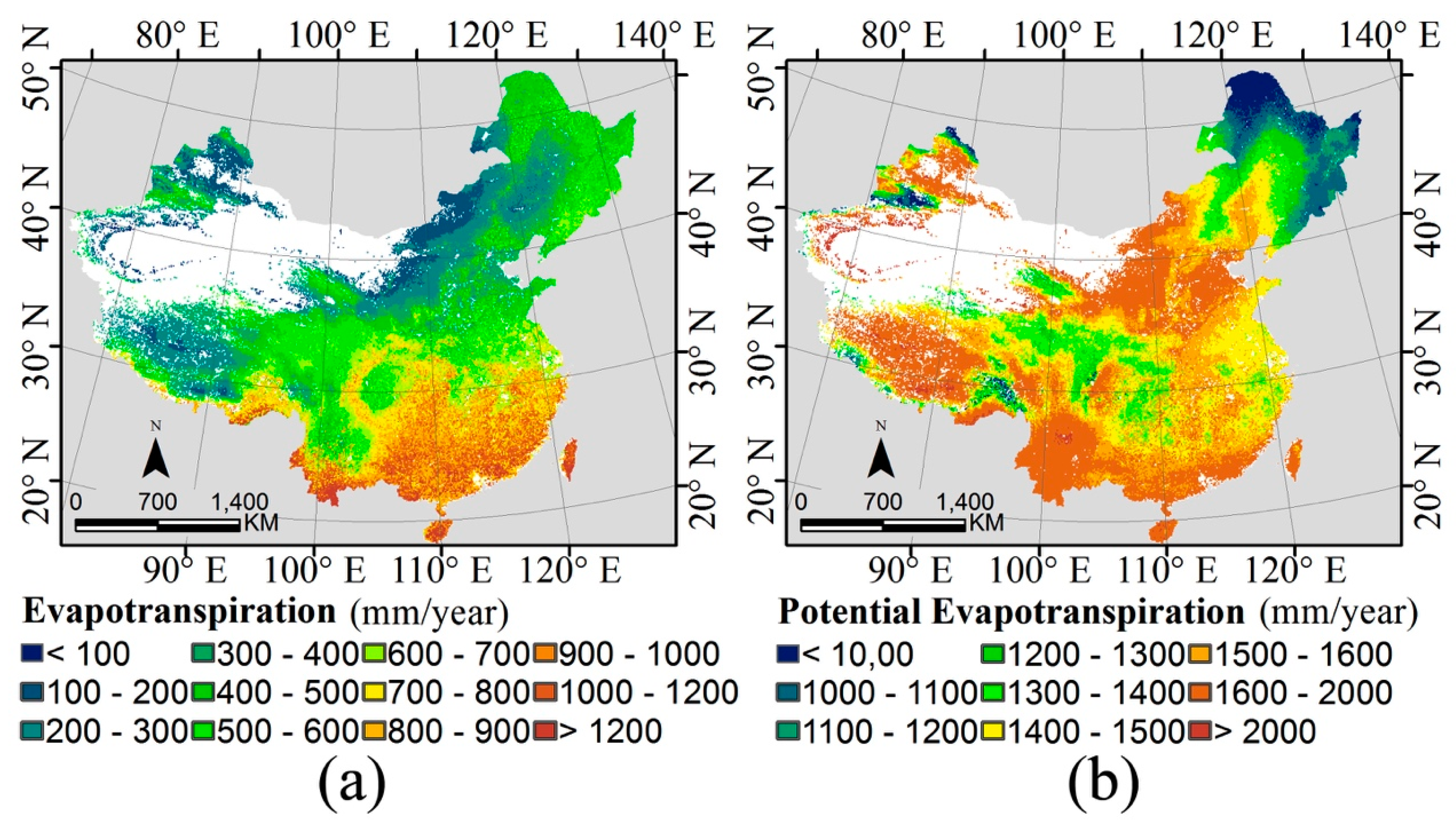
2.1. Water-Energy Dynamics and Remote Sensing Datasets

Potential evapotranspiration (PET) and evapotranspiration (ET) were used to represent the water-energy dynamics of land, considering their vital roles in global climate dynamics and terrestrial ecosystem productivity dynamics [12,14,15,16]. PET and ET represent good predictors of species richness patterns [9] but are not consistent. Currie [17] and Rodriguez [10] found that PET was the best predictor for vertebrate richness across North America and for amphibian richness in Europe. However, ET was found to be a strong predictor for birds in Europe and mammals in South America [9,18]. Therefore, further investigations are necessary to determine the ability of PET and ET to predict species richness.

This study used PET and ET time series datasets from the Moderate Resolution Imaging Spectroradiometer (MODIS, MOD16-MODIS Global Evapotranspiration project, http://www.ntsg.umt.edu/project/mod16). PET and ET datasets (monthly for temporal stability and annually for the long-term mean, from 2000 to 2013) at a 1 × 1 km² spatial resolution were provided as grids (level 4 production) in the Geographic Lat/Lon projection based on WGS-84 datum. MOD16 ET datasets were estimated using an improved ET algorithm [19], which was based on the Penman-Monteith equation. The data processing incorporated weather conditions, land cover, vegetation structure, and other factors [19]. Data in China were validated via flux derived/measured data collected by Liu [20]. To preserve the 10 km spatial resolution of species richness, MOD16 datasets were resampled using the nearest neighbor algorithm.

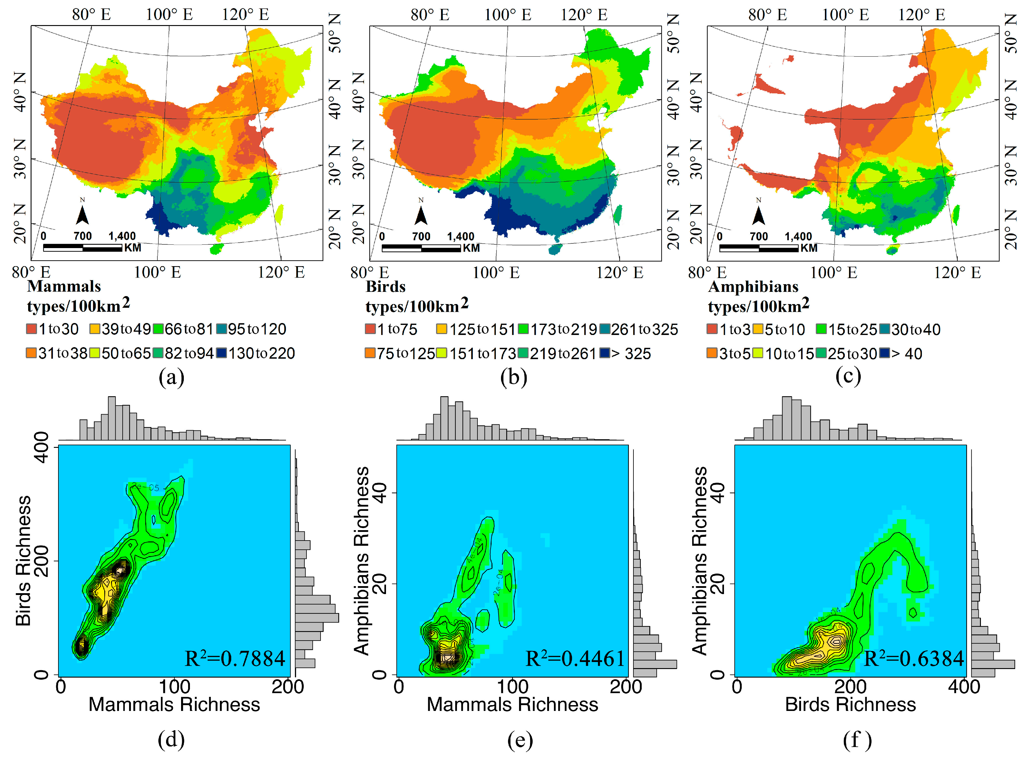
2.2. Species Richness and Remote Sensing Datasets

Census data on the species richness of mammals and amphibians were obtained from the International Union for Conservation of Nature, while census data on birds were obtained from BirdLife International and NatureServe [21,22]. The geographical distribution of mammals was similar to that of birds (R² = 0.7884, Figure 1d). These datasets (Figure 1), which were updated in 2013 at a 10 × 10 km² spatial resolution, were used to test the relationship between the field survey datasets and the water-energy-derived surrogate of species richness based on remote sensing.

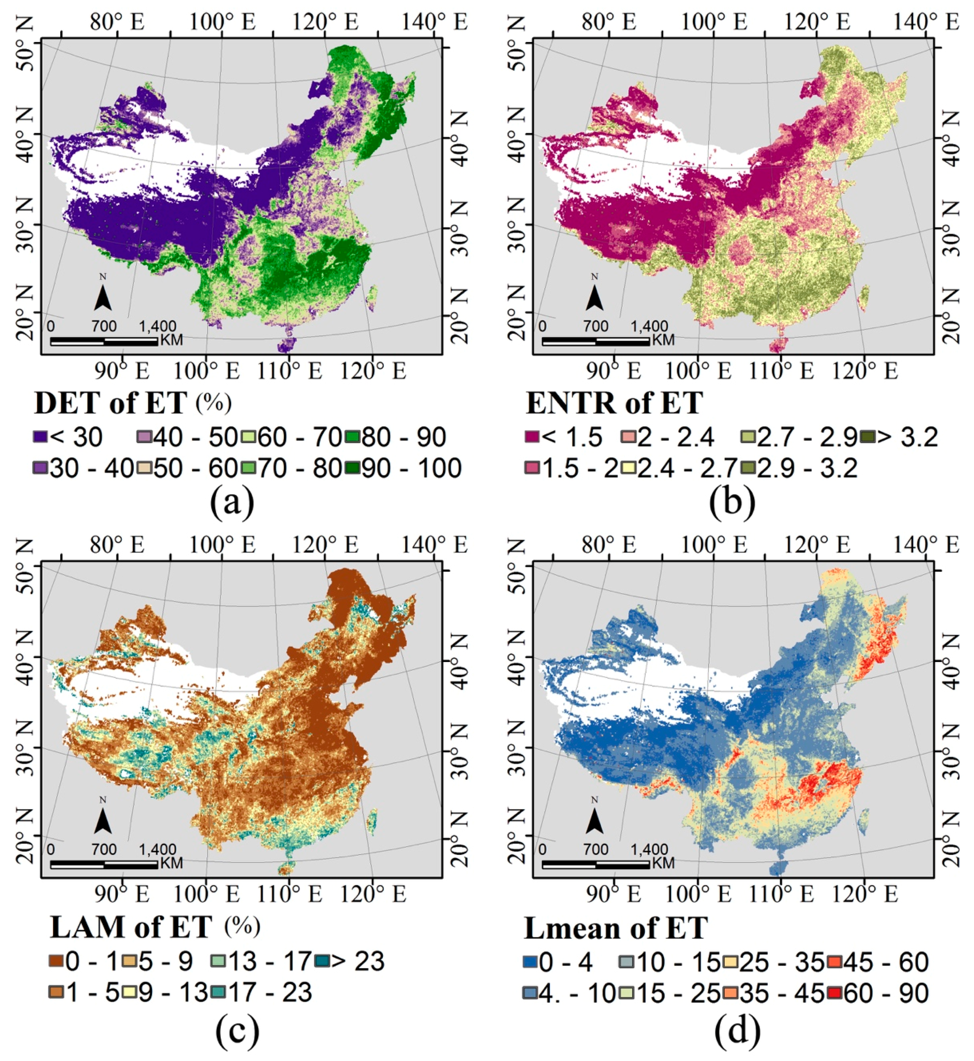
2.3. Indices of Temporal Stability

PET and ET reflect climatic dynamics and how variation therein interacts with the ecosystem. However, climatic dynamics and the ecosystem are inherently non-linear in space and time [13,24]. Thus, it is important to consider how the temporal stability of time series datasets affects species. In this study, determinism (DET), entropy of diagonal length (ENTR), averaged diagonal length (Lmean), and laminarity (LAM) were estimated using recurrence quantification analysis (RQA, for more detail see [25]). These indices have been previously used to characterize time series data obtained from social systems to biological systems [13,24]. Here, these four indices were used to evaluate the temporal stability of the ET series. These four indices are based on the diagonal and vertical line structure of the recurrence plot (RP, which is plotted as a trajectory $\overrightarrow{x_i}\in R^n \left(i=1,\dots ,N\right)$ in the n-dimensional phase space and represent the recurrence of the phase space trajectory to a specific state via a matrix plot, in which white = 0 and black = 1. The two axes in RP represent time [25,26]). In the histograms, the diagonal lines (representing the similar local evolution of different parts of the trajectory) have a length of l, while the vertical lines (indicating an unchanged state for some time) have a length of v in the RP, with the total number following that in [25]:

$$P\left(l\right)={\displaystyle \sum _{i,j=1}^N}\left(1-{\mathrm{R}}_{i-1,j-1}(\mathsf{\epsilon })\right)\left(1-{\mathrm{R}}_{i+l,j+l}(\mathsf{\epsilon })\right){\displaystyle \prod _{k=0}^{v-1}}{\mathrm{R}}_{i+k,j+k}(\mathsf{\epsilon })$$

(1)

$$P\left(v\right)={\displaystyle \sum _{i,j=1}^N}\left(1-{\mathrm{R}}_{i,j}\right)\left(1,{\mathrm{R}}_{i,j+v}\right){\displaystyle \prod _{k=0}^{v-1}}{\mathrm{R}}_{i,j+k}$$

(2)

where $\mathsf{\epsilon }$ is the distance threshold.

DET measures the determinism (predictability) of a given system and is the ratio of recurrence points that form diagonal structures to all recurrence points. DET ranges from 0 to 1, in which values close to 0 represent a random series, while values close to 1 represent a deterministic series [25].

$$DET=\frac{{\sum }_{l=l_{min}}^{N}lP\left(l\right)}{{\sum }_{l=1}^{N}lP\left(l\right)}$$

(3)

ENTR refers to the Shannon entropy of the probability (p(l)) of finding a diagonal line of an exact length l in the RP and reflects the complexity of the RP in relationship with the diagonal lines. High ENTR indicates high complexity [25].

$$N_l={\sum }_{l\ge l_{min}}P\left(l\right)$$

(4)

$$p\left(l\right)=\frac{P\left(l\right)}{N_l}$$

(5)

$$ENTR=-{\displaystyle \sum _{l=l_{min}}^N}p\left(l\right)\ln p\left(l\right)$$

(6)

LAM, named laminarity, is the ratio between the recurrence of points that form the vertical structures and the entire set of recurrence points. LAM measures the amount of laminar states (periodic-chaotic/chaotic-periodic, as well as chaos-chaos transitions) [25,26].

$$LAM=\frac{{\sum }_{v=v_{min}}^{N}vP\left(v\right)}{{\sum }_{v=1}^{N}vP\left(v\right)}$$

(7)

Lmean is the average length of the diagonal line, which is the average time that two segments of the trajectory are near to each other and represents the mean prediction time [25].

$$Lmean=\frac{{\sum }_{l=l_{min}}^{N}lP\left(l\right)}{{\sum }_{l=l_{min}}^{N}P\left(l\right)}$$

(8)

DET, ENTR, and Lmean are indices that are based on the diagonal lines produced by recurrence plots. DET and ENTR indicate the structure and complexity level of time series data. High DET values indicate that the data in a given time series have a determinant structure, regardless of structure type. However, a complex structure usually has high ENTR values. LAM is sensitive to transitions, with a higher value representing more frequent transitions between laminar states [25,26]. Lmean represents the mean prediction time when two segments of a trajectory are close to each other at different times [25].

2.4. Tendency Analysis

Trends were analyzed with gridded data on the possible predictors of species richness to explore the potential causes of the observed changes. To estimate long-term PET and ET dynamics (2000–2013), a simple linear regression analysis by least squares [27] was applied to annual PET and ET.

$$Slope=\frac{\mathrm{T}\times {\sum }_{{\mathrm{t}}_s}^{{\mathrm{t}}_e}\mathrm{t}\times \mathrm{DN}-\left({\sum }_{{\mathrm{T}}_s}^{{\mathrm{t}}_e}\mathrm{t}\right)\left({\sum }_{{\mathrm{t}}_s}^{{\mathrm{t}}_e}\mathrm{DN}\right)}{\mathrm{T}\times {\sum }_{{\mathrm{t}}_s}^{{\mathrm{t}}_e}{\mathrm{t}}^2-{\left({\sum }_{{\mathrm{t}}_s}^{{\mathrm{t}}_e}\mathrm{t}\right)}^2}$$

(9)

where t ∈ {2000, 2001,…, 2013} represents the specific year, T is the number of total years, and DN is the digital number of PET or ET grid cells for a particular year. The trend of PET or ET increases when Slope is positive, and vice versa. This analysis was conducted using the functio‘REGRESS’ in IDL©6.4 (Interactive Data Language) and ENVI©4.4 (Environment for Visualizing Images).

2.5. Statistical Analysis

Transforming the monthly time series data to indices of temporal stability is a key step for determining the ability of temporal stability to predict species richness. A direct linear relationship between the long-term mean of time-series datasets and particular species richness has been previously documented [9]; however, few studies have reported the temporal stability of long-term time series datasets. Here, we tested the hypothesis that PET, ET, or temporal stability constitutes reliable surrogates of species richness at moderate energy regimes, where PET > 1000 mm/year, allowing the classification of species richness in large areas (and how it changes through time) based on a simple linear regression model. The model equation was as follows; species richness = a × (ET or PET or Temporal stability indices) + b, where a is the slope of the regression line and b is the y-intercept. A linear relationship was confirmed from the R² and p-value of the regression, indicating that it is a good predictor of a possible remote sensing surrogate for species richness.

Step 1: Data-preprocessing: IDL© 6.4 and ENVI©4.4 software were used to relate/combine and resample MODIS PET and ET data (1 × 1 km²) to obtain a suitable spatial resolution of 10 × 10 km² for the actual field surveys of species abundance.

Step 2: Use of the long-term PET or ET mean to predict species richness: The long-term means of PET and ET (based on annual datasets from 2000 to 2013) were compared with the field survey data of species richness to analyze their potential as remote sensing water-energy dynamics proxies for predicting species richness by employing simple linear regression (conducted using the ‘stats’ package in R).

Step 3: Effects of temporal stability on species richness: Among long-term means, ET shows a good ability to predict species richness. Thus, we extracted the indices of temporal stability based on monthly ET datasets. The values (12 months × 14 years) of each pixel were transformed into a unique file format (text) to obtain the four indices (DET, ENTR, LAM, and Lmean) of temporal stability using the CRT Toolbox for Matlab by Norbert Marwan [25]. These indices were transformed back from points to the grid datasets. The parameters of RQA were determined from the mean ET value across China: embedding dimension m = 6 (determined by the false nearest neighbors [28] and the Cao method [29]); and time delay τ = 2 (determined via the mutual information method [30]). The 10% of the maximum phase space diameter [25] was chosen as the threshold ε for each pixel. These four indices were used to test the assumption that temporal stability is a viable surrogate for species richness at the regional scale, based on simple linear regression (conducted with the ‘stats’ package in R program).

Step 4: Tendency analysis: Changes in water-energy dynamics over time were conducted based on annual time series datasets (as demonstrated in Section 2.4) using IDL© 6.4 and ENVI©4.4 software.

3. Results and Discussion

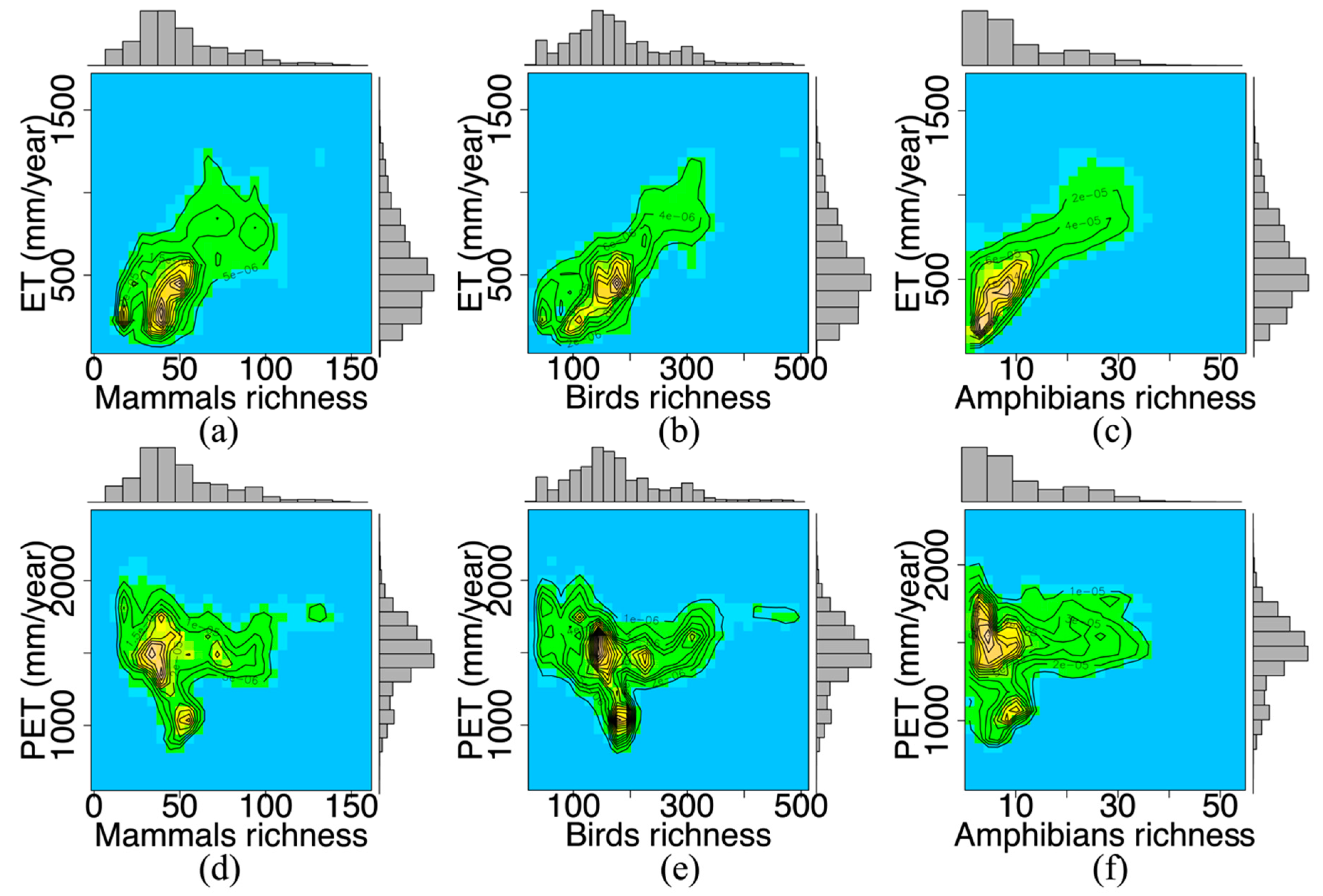
3.1. The Water-Energy Dynamics and Species Richness

The geographical distribution of ET and PET differed across China, showing high heterogeneity (Figure 2). Our results show that China is dominated by a moderate energy regime, with PET > 1000 mm/year. Low energy regimes were mainly found in the northern part of the Northeast China Plain. ET exhibited high radiation in southeast China and northwest China but was wet in the former and dry in the latter with grassland. However, the low-altitude regions on the Tibetan Plateau in the prefectures of Shannan and Linzhi were covered with rainforests and also had high ET values. No obvious linear relationship was detected between ET and PET.

To determine the relationship between species richness from the field survey (Figure 1) and long-term averaged ET and PET, frequency distributions and linear regressions were used. Species richness appeared to be strongly and positively correlated with ET patterns, with R² ∈ (0.40~0.67), especially for amphibians (R² ~ 0.6639). For more details, see Figure 3 and

Table 1. Correlation coefficients of species richness based on field surveys versus remote sensing-based ET and PET using a simple linear regression of raw data.

Species Richness	Slopes		R2		p Value	DF
	ET	PET	ET	PET
Mammals	0.0617	0.0030	0.4028	0.004	<0.05	65,135
Birds	0.2517	0.0063	0.5735	0.003	<0.05	65,135
Amphibians	0.0288	0.0740	0.6639	0.0352	<0.05	54,738

. In addition, the consistency of these results was examined using an ERA-Interim ET dataset. However, species richness had a much lower correlation with PET than expected (R² < 0.1, see Table 1). Therefore, our results indicate that ET, rather than PET, based on the remote sensing of the water-energy dynamics, represents a reliable surrogate of species richness, at least for mammals, birds, and amphibians, in the moderate energy regime of China (that is, PET > 1000 mm/year).

In comparatively cold regions, energy is an important limitation for the geographical distribution of species because it constrains resources, affecting physiological requirements and reproduction, among other factors [31,32]. Therefore, PET effectively predicts species richness gradients in relatively low energy areas (PET < 1000 mm/year). However, as energy increases in moderate energy regimes, water availability, or the interaction between water and energy, is pivotal [31]. Consequently, ET better explains species richness in China than does PET. This analysis of terrestrial species richness in China strongly supports the water-energy hypothesis [4].

Our finding that amphibians are sensitive to the long-term mean of the ET time series supports a previous study on the relative sensitivity of species in the northwestern part of North America to climate change [2]. Our results also support those of Qian [33], who concluded that water and energy are the primary explanatory variables for amphibians. The different physiological requirements (e.g., amphibians usually require water for habitat-use and reproduction) and evolutionary processes among amphibians, mammals, and birds [33] appear to be the primary factors influencing the sensitivity of the species belonging to these different groups to climate change.

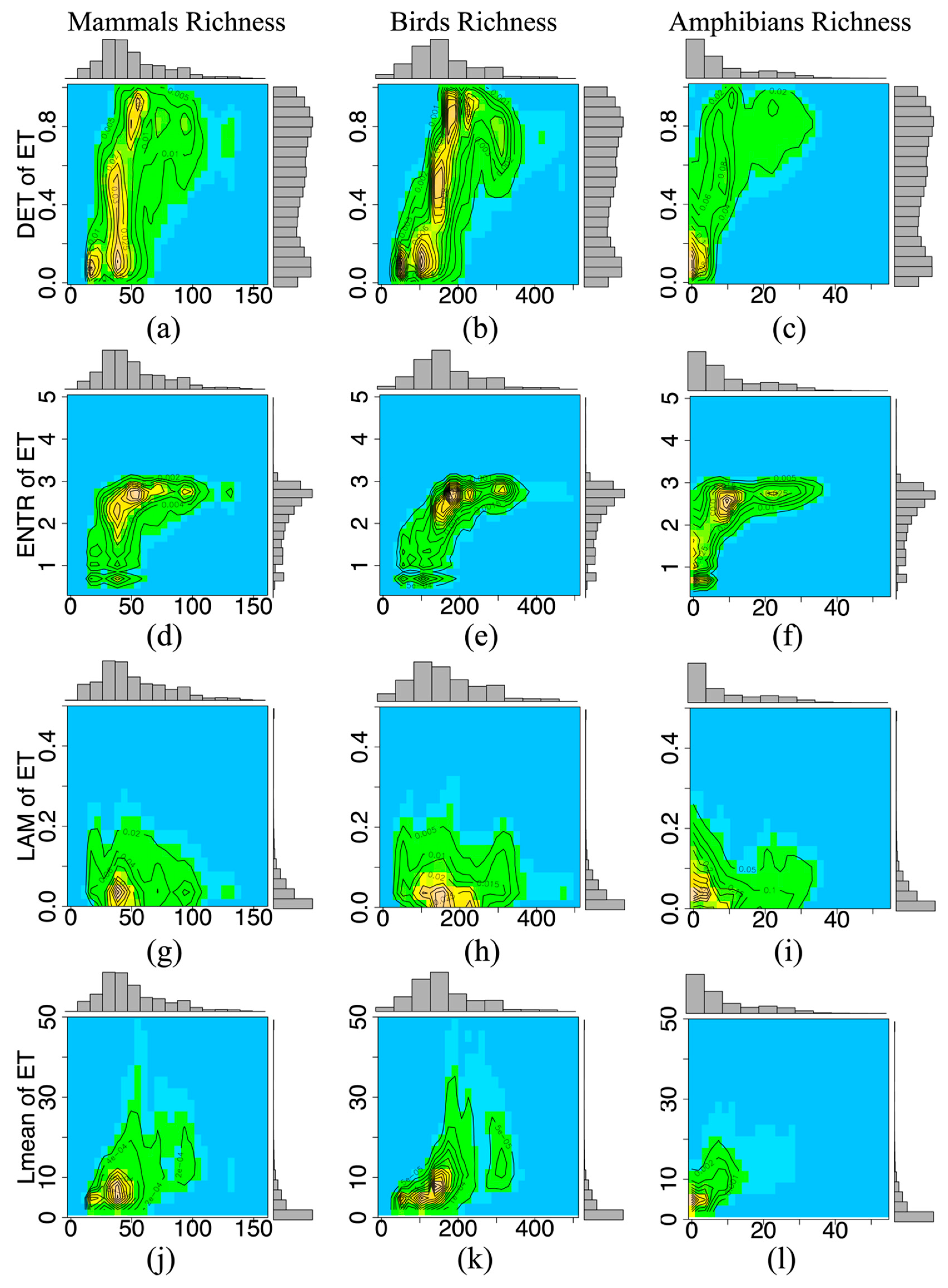
3.2. Temporal Stability and Species Richness

The spatial patterns of DET, ENTR, LAM, and Lmean show clear spatial heterogeneity and similar regional distributions (except for LAM, Figure 4). These patterns were associated with vegetation cover (evergreen forest > deciduous forest > cropland > grassland). Higher DET (ENTR and Lmean) occurs in the mountains of southern China, which are covered in evergreen broad-leaf forests; the Northeast China Plain, which is covered in evergreen needle-leaf forests; and the southern part of the Qinghai-Tibet Plateau, which is covered in tropical forests. The ET time series in these regions appeared to be more stable in these regions. Lower DET values were found in northwest China and on the Qinghai-Tibet Plateau, which were covered with grassland or sparse vegetation. The ET time series was more stochastic in these regions. LAM is sensitive to disturbance. Relatively high LAM occurred in the southern coastal areas, in addition to the Qinghai-Tibet Plateau, the Loess Plateau, and the Northeast China Plain. These results were consistent with ET and PET trends, indicating that these areas have changed over time.

Higher DET, ENTR, and Lmean values indicate that temporal stability is stable and determinate (lack of disturbance) when species richness is higher. Species richness was positively correlated with the temporal stability of ET in a monthly time series, especially when species richness was low. However, the presence of asymptotic relationships (Figure 5a–f) indicates that certain underlying factors (except for DET and ENTR) affect species richness when both water levels and energy are high.

For objective comparison, the relationships between species richness and the indices of temporal stability were also examined by simple linear regression using the original data. Unexpectedly, the long-term mean of ET was more strongly correlated with species richness than the indices of temporal stability (

Table 2. Correlation coefficients between the species richness from field surveys and the temporal stability of ET using a simple linear regression of the raw data.

Species Richness	R2				p Value	DF
	DET	ENTR	LAM	Lmean
Mammals	0.2493	0.2332	0.0001	0.1276	<0.05	65,135
Birds	0.3564	0.3643	0.0007	0.1758	<0.05	65,135
Amphibians	0.3106	0.2840	0.0039	0.2053	<0.05	54,738

). The relationship between species and temporal stability for the three taxonomic groups produced similar patterns (Figure 5), extending from no correlation (species vs LAM) to weakly linear (species vs Lmean), with some asymptotic cases (species vs DET and ENTR). All of the results suggest that the climate mean of ET explains species richness better than the indices of temporal stability. In contrast, areas with high DET, ENTR, and Lmean supported a high level of species richness. However, species richness was better explained when the indices of temporal stability were combined with the climate mean of ET (

Table 3. Correlation coefficients of species richness, based on field surveys, versus temporal stability incorporated with the long-term mean of ET using the simple linear regression of the raw data.

Variations	R2
	Mammals	Birds	Amphibians
DET	0.4250	0.6057	0.6794
DET + ENTR	0.4301	0.6132	0.6859
DET + ENTR + LAM	0.4302	0.6137	0.6860
DET + ENTR + LAM + Lmean	0.4357	0.6234	0.6882
DET + ENTR + Lmean	0.4357	0.6231	0.6881

). Species often show different responses to the temporal stability of the climate due to different species interacting differently with their environment [13] and different evolutionary responses [34]; consequently, the relative sensitivity of species to climate change varies within different taxonomic groups [2].

The temporal stability of ET is primarily associated with climate perturbations and changes. Landscape structure and vegetation diversity also contribute to differences in temporal stability [35]. Areas with low temporal stability (measured by DET, ENTR, LAM, and Lmean) vary more over time. Spatial variability indicates greater environmental heterogeneity, providing more opportunities for the coexistence of species that have higher resilience to perturbations [36,37,38]. However, species are likely to show different responses to changes in climate and habitat with respect to space use (geographical distribution) and individual traits (physiological, e.g., behavior transforming). Therefore, specialist species are more prone to extinction under the influence of these changes [1,39,40].

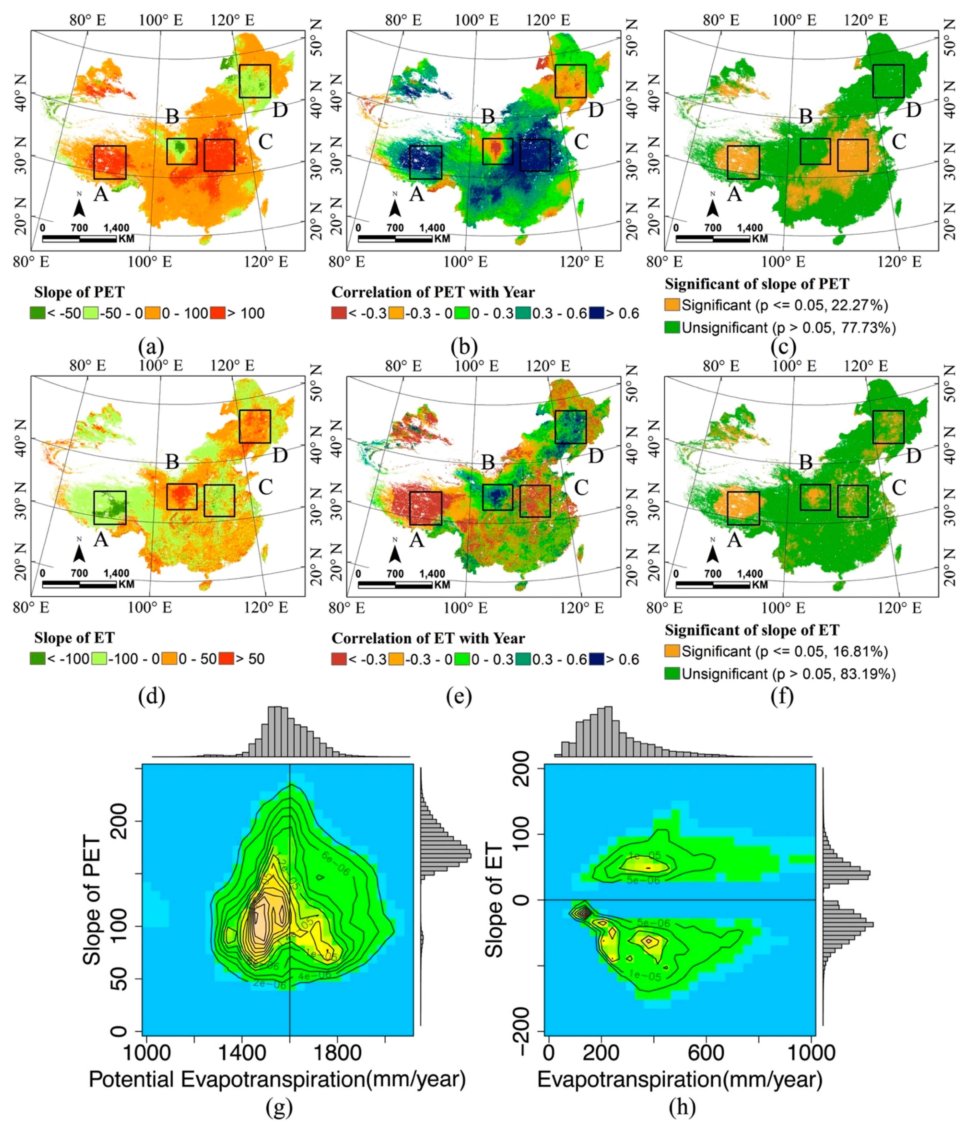
3.3. Tendency and Change

Previous studies suggested that the warming climate and changing precipitation patterns have induced changes in ET and PET in addition to biodiversity [1,41]. To determine whether such trends persist over the long-term (2000–2013) for PET and ET, simple linear regression analyses were implemented to determine the slope, correlation, and significance (Figure 6a–f). Four sub regions (the Qinghai-Tibet Plateau, the Loess Plateau, the North China Plain, and the Northeast China Plain) were highlighted due to the strong PET and ET trends, as well as the regional differences in climate, land cover, species richness, and threatened species richness. Three key results were detected.

First, the maximum slopes of increasing in PET and decreasing in ET occur in the North China Plain (Frame C in Figure 6) and the Qinghai-Tibet Plateau (Figure 6, Frame A). Both increasing temperature and changing patterns in precipitation contributed to changes on the Qinghai-Tibet Plateau, where precipitation increased in the west but decreased in the south [42,43,44]. Similar patterns were recorded on the North China Plain, where precipitation increased in winter but decreased in summer [45]. A changing pattern in wet-dry periods was recorded for the Qinghai-Tibet Plateau [42,43]. In comparison, increasing rainfall infiltration caused changes on the North China Plain [46].

Second, a significant increase in ET was detected in the Losses Plateau (p < 0.05; Figure 6, Frame B). In comparison, there was no significant (p > 0.05) decrease in PET on the plateau due to the implementation of the Grain-to-Green Program since 1999 [47,48]. The transpiration of water by vegetation increased due to reforestation, causing the vegetation coverage on the Loess Plateau to increase from 31.6% in 1999 to 59.6% in 2013 [49]. The combination of the warming climate and decreasing precipitation in the southeastern part of the Loess Plateau (based on data from meteorological stations, which corresponded to increased vegetation cover) [50,51] will lead to an increased severity of droughts in the surface layer, which will threaten biodiversity by reducing productivity, leading to ecological degradation [1,49].

Third, a significant increase in ET with no obvious change in PET was detected in the Northeast China Plain (Figure 6, Frame D). The dominant factors contributing to this phenomenon include increasing temperature and decreasing precipitation (especially in summer) [52]. Moreover, land cover change, such as converting wheat or bean production to rice production, also contributed to increased ET [53].

A comparison between ET and PET and the relationship between them were investigated for the areas with significant changes (i.e., areas with p-values ≤ 0.05 and |R| > 0.5). Significant changes in ET and PET occurred in 16.81% and 22.27% of the total area, respectively. The relationship of PET with the slope changed when PET was greater or smaller than 1600 mm/year. For instance, the slope was positively correlated to PET when PET was <1600 mm/year but was negatively related to PET when PET was >1600 mm/year. Both increasing and decreasing trends of ET were more obvious when the values of ET were high.

Both climate change and anthropogenic activity contribute to PET and ET trends, affecting the spatial distribution of species and populations. PET and ET trends respond well to climate change, including changes in precipitation patterns and increasing temperature. The analysis based on climate stations coincided with the change in ET and PET on the Qinghai-Tibet Plateau [52]. The pan evaporation data derived from the stations in each region showed that ET significantly decreased in the Qinghai-Tibet Plateau and the North China Plain but increased in the Northeast China Plain and the Loess Plateau [52]. Moreover, disruptions to the ecosystem, such as deforestation and land use conversion over large regions, were detected from significant trends in ET. Positive human restoration activities, such as Grain-to-Green, the National Forest Conversation Program, and Shelter Forest, also significantly influence ET by changing the vegetation cover and water-cycle [54].

Uncertainty exists due to knowledge of the geographical distribution of known species remaining limited, even though most species are considered to have been described [55]. For example, the distribution of mammals across China [56] is not consistent with the distribution on the global map [21]. Furthermore, people’s understanding of species differs [55], with genus and species richness being constantly updated as access to new technologies improves. New technologies, such as DNA bar-coding [57] and crowd-sourced data [58], offer substantial opportunities to identify and monitor a broad range of species over time and across large geographical regions. In addition, the accuracy of remote sensing data (e.g., inaccurate measures of ET in the Tibetan Plateau, which was not the focus of the current study) needs to be considered, with corrected data being integrated to improve its ability to predict the species richness. An accurate database on the geographical distribution of species would enhance biodiversity conservation but requires major effort to be realized.

4. Conclusions

In summary, this study is the first to apply the water-energy hypothesis to China, allowing comparison with results previously obtained for North America, Europe, and southern Africa. Furthermore, we extended the hypothesis from using just the long-term mean of ET to include the temporal stability of ET too. As a result, we demonstrated how the long-term mean and temporal stability of ET based on remote sensing are correlated with species richness using RQA and linear regression.

We confirmed that ET is a better predictor of species richness than PET in China, which has moderate energy (that is, PET > 1000 mm/year), especially for amphibians. Compared with temporal stability, the long-term mean of ET also explained species richness better. Both climate and anthropogenic changes contribute to the observed trends in ET and PET time series. The warming climate and the change in precipitation showed significant changes to ET and PET, which, in turn, affect biodiversity. Furthermore, the restoration of natural vegetation and changes in land cover alter the dynamics of water and energy, as well as biodiversity. Water-energy dynamics and their temporal stability clearly affect species richness. Areas with high water and energy, as well as determinate and regular climate systems, support relatively high levels of species richness.

These results improve our understanding of the water-energy dynamics and the spatial-temporal dynamics of terrestrial biodiversity in China, allowing the influence of climate change and anthropogenic change to be considered. We monitored these effects by detecting trends in ET and PET based on remote sensing. The impacts of climate change (including warming temperature and changing precipitation patterns) are the primary factors that constrain the water-energy balance in China. Regions with human activities (including land cover change and reforestation) have mainly contributed to changes in ET and PET in the Northeast China Plain and the Loess Plateau. Therefore, future aims to protect the climate by regulating water-energy dynamics through land management and reforestation should be considered when planning the conservation of natural resources, which would, in turn, protect biodiversity.

References

1. Mantyka-pringle, C.S.; Martin, T.G.; Rhodes, J.R. Interactions between climate and habitat loss effects on biodiversity: A systematic review and meta-analysis. Glob. Chang. Biol. 2012, 18, 1239–1252. [Google Scholar] [CrossRef]
2. Case, M.J.; Lawler, J.J.; Tomasevic, J.A. Relative sensitivity to climate change of species in northwestern North America. Biol. Conserv. 2015, 187, 127–133. [Google Scholar] [CrossRef]
3. Fritz, S.A.; Bininda-Emonds, O.R.; Purvis, A. Geographical variation in predictors of mammalian extinction risk: Big is bad, but only in the tropics. Ecol. Lett. 2009, 12, 538–549. [Google Scholar] [CrossRef] [PubMed]
4. Hawkins, B.A.; Field, R.; Cornell, H.V.; Currie, D.J.; Guégan, J.-F.; Kaufman, D.M.; Kerr, J.T.; Mittelbach, G.G.; Oberdorff, T.; O’Brien, E.M. Energy, water, and broad-scale geographic patterns of species richness. Ecology 2003, 84, 3105–3117. [Google Scholar] [CrossRef]
5. Zhang, K.; Kimball, J.S.; Mu, Q.; Jones, L.A.; Goetz, S.J.; Running, S.W. Satellite based analysis of Northern ET trends and associated changes in the regional water balance from 1983 to 2005. J. Hydrol. 2009, 379, 92–110. [Google Scholar] [CrossRef]
6. O’Brien, E.M. Biological relativity to water–energy dynamics. J. Biogeogr. 2006, 33, 1868–1888. [Google Scholar] [CrossRef]
7. O’Brien, E. Water-energy dynamics, climate, and prediction of woody plant species richness: An interim general model. J. Biogeogr. 1998, 25, 379–398. [Google Scholar] [CrossRef]
8. Gillman, L.N.; Wright, S.D.; Cusens, J.; McBride, P.D.; Malhi, Y.; Whittaker, R.J. Latitude, productivity and species richness. Glob. Ecol. Biogeogr. 2015, 24, 107–117. [Google Scholar] [CrossRef]
9. Hawkins, B.A.; Porter, E.E. Relative influences of current and historical factors on mammal and bird diversity patterns in deglaciated North America. Glob. Ecol. Biogeogr. 2003, 12, 475–481. [Google Scholar] [CrossRef]
10. Rodriguez, M.A.; Belmontes, J.A. Energy, water and large-scale patterns of reptile and amphibian species richness in Europe. Acta Oecol. 2005, 28, 65–70. [Google Scholar] [CrossRef]
11. Whittaker, R.J.; Nogués-Bravo, D.; Araújo, M.B. Geographical gradients of species richness: A test of the water-energy conjecture of Hawkins et al. (2003) using European data for five taxa. Glob. Ecol. Biogeogr. 2007, 16, 76–89. [Google Scholar] [CrossRef]
12. Currie, D.J.; Mittelbach, G.G.; Cornell, H.V.; Field, R.; Guégan, J.F.; Hawkins, B.A.; Kaufman, D.M.; Kerr, J.T.; Oberdorff, T.; O’Brien, E. Predictions and tests of climate-based hypotheses of broad-scale variation in taxonomic richness. Ecol. Lett. 2004, 7, 1121–1134. [Google Scholar] [CrossRef]
13. Proulx, R.; Parrott, L.; Fahrig, L.; Currie, D.J. Long time-scale recurrences in ecology: Detecting relationships between climate dynamics and biodiversity along a latitudinal gradient. In Recurrence Quantification Analysis; Springer: Berlin, Germany, 2015; pp. 335–347. [Google Scholar]
14. Bini, L.M.; Diniz-Filho, J.A.F.; Hawkins, B.A. Macroecological explanations for differences in species richness gradients: A canonical analysis of South American birds. J. Biogeogr. 2004, 31, 1819–1827. [Google Scholar] [CrossRef]
15. Alemu, H.; Senay, G.B.; Kaptue, A.T.; Kovalskyy, V. Evapotranspiration variability and its association with vegetation dynamics in the Nile Basin, 2002–2011. Remote Sens. 2014, 6, 5885–5908. [Google Scholar] [CrossRef]
16. Thomas, A. Spatial and temporal characteristics of potential evapotranspiration trends over China. Int. J. Climatol. 2000, 20, 381–396. [Google Scholar] [CrossRef]
17. Currie, D.J. Energy and large-scale patterns of animal-and plant-species richness. Am. Nat. 1991, 137, 27–49. [Google Scholar] [CrossRef]
18. Ruggiero, A.; Kitzberger, T. Environmental correlates of mammal species richness in South America: Effects of spatial structure, taxonomy and geographic range. Ecography 2004, 27, 401–417. [Google Scholar] [CrossRef]
19. Mu, Q.; Zhao, M.; Running, S.W. Improvements to a MODIS global terrestrial evapotranspiration algorithm. Remote Sens. Env. 2011, 115, 1781–1800. [Google Scholar] [CrossRef]
20. Liu, Z.; Shao, Q.; Liu, J. The performances of MODIS-GPP and-ET products in China and their sensitivity to input data (fPAR/LAI). Remote Sens. 2014, 7, 135–152. [Google Scholar] [CrossRef]
21. Jenkins, C.N.; Pimm, S.L.; Joppa, L.N. Global patterns of terrestrial vertebrate diversity and conservation. Proc. Natl. Acad. Sci. USA 2013, 110, 2602–2610. [Google Scholar] [CrossRef] [PubMed]
22. Pimm, S.L.; Jenkins, C.N.; Abell, R.; Brooks, T.M.; Gittleman, J.L.; Joppa, L.N.; Raven, P.H.; Roberts, C.M.; Sexton, J.O. The biodiversity of species and their rates of extinction, distribution, and protection. Science 2014. [Google Scholar] [CrossRef] [PubMed]
23. Zhang, C.; Cai, D.; Guo, S.; Guan, Y.; Fraedrich, K.; Nie, Y.; Liu, X.; Bian, X. Spatial-temporal dynamics of China’s terrestrial biodiversity: A dynamic habitat index diagnostic. Remote Sens. 2016, 8, 227. [Google Scholar] [CrossRef]
24. Parrott, L. Measuring ecological complexity. Ecol. Indic. 2010, 10, 1069–1076. [Google Scholar] [CrossRef]
25. Marwan, N.; Romano, M.C.; Thiel, M.; Kurths, J. Recurrence plots for the analysis of complex systems. Phys. Rep. 2007, 438, 237–329. [Google Scholar] [CrossRef]
26. Marwan, N.; Wessel, N.; Meyerfeldt, U.; Schirdewan, A.; Kurths, J. Recurrence-plot-based measures of complexity and their application to heart-rate-variability data. Phys. Rev. E 2002, 66, 026702. [Google Scholar] [CrossRef] [PubMed]
27. Rao, C.R.; Toutenburg, H.; Shalabh, H.C.; Schomaker, M. Linear Models and Generalizations. Least Squares and Alternatives, 3rd ed.; Springer: Berlin, Germany, 2008. [Google Scholar]
28. Abarbanel, H.D.; Brown, R.; Sidorowich, J.J.; Tsimring, L.S. The analysis of observed chaotic data in physical systems. Rev. Mod. Phys. 1993, 65, 1331. [Google Scholar] [CrossRef]
29. Cao, L. Practical method for determining the minimum embedding dimension of a scalar time series. Physica D 1997, 110, 43–50. [Google Scholar] [CrossRef]
30. Fraser, A.M.; Swinney, H.L. Independent coordinates for strange attractors from mutual information. Phys. Rev. A 1986, 33, 1134. [Google Scholar] [CrossRef]
31. Qian, H.; Kissling, W.D. Spatial scale and cross-taxon congruence of terrestrial vertebrate and vascular plant species richness in China. Ecology 2010, 91, 1172–1183. [Google Scholar] [CrossRef] [PubMed]
32. Kerr, J.T.; Packer, L. Habitat heterogeneity as a determinant of mammal species richness in high-energy regions. Nature 1997, 385, 252–254. [Google Scholar] [CrossRef]
33. Qian, H.; Wang, X.; Wang, S.; Li, Y. Environmental determinants of amphibian and reptile species richness in China. Ecography 2007, 30, 471–482. [Google Scholar] [CrossRef]
34. Hawkins, B.A.; McCain, C.M.; Davies, T.J.; Buckley, L.B.; Anacker, B.L.; Cornell, H.V.; Damschen, E.I.; Grytnes, J.A.; Harrison, S.; Holt, R.D. Different evolutionary histories underlie congruent species richness gradients of birds and mammals. J. Biogeogr. 2012, 39, 825–841. [Google Scholar] [CrossRef]
35. Zhao, Z.; Liu, J.; Peng, J.; Li, S.; Wang, Y. Nonlinear features and complexity patterns of vegetation dynamics in the transition zone of North China. Ecol. Indic. 2015, 49, 237–246. [Google Scholar] [CrossRef]
36. Fjeldså, J.; Bowie, R.C.K.; Rahbek, C. The role of mountain ranges in the diversification of birds. Annu. Rev. Ecol. Evol. Syst. 2012, 43, 249–265. [Google Scholar] [CrossRef]
37. Hortal, J.; Carrascal, L.M.; Triantis, K.A.; Thébault, E.; Meiri, S.; Sfenthourakis, S. Species richness can decrease with altitude but not with habitat diversity. Proc. Natl. Acad. Sci. USA 2013, 110, 2149–2150. [Google Scholar] [CrossRef] [PubMed]
38. Tews, J.; Brose, U.; Grimm, V.; Tielbörger, K.; Wichmann, M.C.; Schwager, M.; Jeltsch, F. Animal species diversity driven by habitat heterogeneity/diversity: The importance of keystone structures. J. Biogeogr. 2004, 31, 79–92. [Google Scholar] [CrossRef]
39. Coristine, L.E.; Kerr, J.T. Temperature-related geographical shifts among passerines: Contrasting processes along poleward and equatorward range margins. Ecol. Evol. 2015, 5, 5162–5176. [Google Scholar] [CrossRef]
40. Thomas, C.D. Climate, climate change and range boundaries. Divers. Distrib. 2010, 16, 488–495. [Google Scholar] [CrossRef]
41. Thuiller, W. Biodiversity: Climate change and the ecologist. Nature 2007, 448, 550–552. [Google Scholar] [CrossRef] [PubMed]
42. Cai, D.; Fraedrich, K.; Sielmann, F.; Zhang, L.; Zhu, X.; Guo, S.; Guan, Y. Vegetation dynamics on the Tibetan Plateau (1982 to 2006): An attribution by eco-hydrological diagnostics. J. Clim. 2015, 4576–4584. [Google Scholar] [CrossRef]
43. Chen, H.; Zhu, Q.; Peng, C.; Wu, N.; Wang, Y.; Fang, X.; Gao, Y.; Zhu, D.; Yang, G.; Tian, J.; et al. The impacts of climate change and human activities on biogeochemical cycles on the Qinghai-Tibetan Plateau. Glob. Chang. Biol. 2013, 19, 2940–2955. [Google Scholar] [CrossRef] [PubMed]
44. Wang, M.; Zhou, C.; Wu, L. Aridity pattern of Tibetan Plateau and its influential factors in 2001–2010. Adv. Clim. Chang. Res. 2012, 8, 320–326. [Google Scholar]
45. Fan, L.; Lu, C.; Yang, B.; Chen, Z. Long-term trends of precipitation in the North China Plain. J. Geogr. Sci. 2012, 22, 989–1001. [Google Scholar] [CrossRef]
46. Meng, S.; Fei, Y.; Zhang, Z.; Lei, T.; Qian, Y.; Li, Y. Research on spatial and temporal distribution of the precipitation infiltration amount over the past 50 years in North China Plain. Adv. Earth Sci. 2013, 8, 9. [Google Scholar]
47. Uchida, E.; Xu, J.; Rozelle, S. Grain for green: Cost-effectiveness and sustainability of China’s conservation set-aside program. Land Econ. 2005, 81, 247–264. [Google Scholar] [CrossRef]
48. Xu, Z.; Xu, J.; Deng, X.; Huang, J.; Uchida, E.; Rozelle, S. Grain for green versus grain: Conflict between food security and conservation set-aside in China. World Dev. 2006, 34, 130–148. [Google Scholar] [CrossRef]
49. Chen, Y.; Wang, K.; Lin, Y.; Shi, W.; Song, Y.; He, X. Balancing green and grain trade. Nat. Geosci. 2015, 8, 739–741. [Google Scholar] [CrossRef]
50. Li, Z.; Zheng, F.L.; Liu, W.Z.; Flanagan, D.C. Spatial distribution and temporal trends of extreme temperature and precipitation events on the Loess Plateau of China during 1961–2007. Quatern. Int. 2010, 226, 92–100. [Google Scholar] [CrossRef]
51. Wang, Q.; Fan, X.; Wang, M. Precipitation trends during 1961–2010 in the Loess Plateau region of China. Acta Ecol. Sin. 2011, 31, 5512–5523. [Google Scholar]
52. Qi, T.; Zhang, Q.; Wang, Y.; Xiao, M.; Liu, J.; Sun, P. Spatiotemporal patterns of pan evaporation in 1960–2005 in China: Changing properties and possible causes. Sci. Geograp. Sin. 2015, 35, 1599–1606. [Google Scholar]
53. Liu, J.; Kuang, W.; Zhang, Z.; Xu, X.; Qin, Y.; Ning, J.; Zhou, W.; Zhang, S.; Li, R.; Yan, C. Spatiotemporal characteristics, patterns, and causes of land-use changes in China since the late 1980s. J. Geogr. Sci. 2014, 24, 195–210. [Google Scholar] [CrossRef]
54. He, T.; Shao, Q. Spatial-temporal variation of terrestrial evapotranspiration in China from 2001 to 2010 using MOD16 products. J. Geo-Inform. Sci 2014, 16, 979–988. [Google Scholar]
55. Mayden, R.L. A hierarchy of species concepts: The denouement in the saga of the species problem. In Species: The Units of Biodiversity; Claridge, M.F., Dawah, H.A., Wilson, M.R., Eds.; Chapman and Hall: London, UK, 1997; Volume 54, pp. 381–423. [Google Scholar]
56. Jiang, Z.; Ma, Y.; Wu, Y.; Wang, Y.; Zhou, K.; Liu, S.; Feng, Z.; Li, L. China’s Mammals Diversity and Geographic Distribution; China Science Publishing: Beijing, China, 2015. (In Chinese) [Google Scholar]
57. Hebert, P.D.; Cywinska, A.; Ball, S.L. Biological identifications through DNA barcodes. Proc. R Soc. Lond B Bio. Sci. 2003, 270, 313–321. [Google Scholar] [CrossRef] [PubMed]
58. Fritz, S.; McCallum, I.; Schill, C.; Perger, C.; See, L.; Schepaschenko, D.; van der Velde, M.; Kraxner, F.; Obersteiner, M. Geo-wiki: An online platform for improving global land cover. Environ. Model. Softw. 2012, 31, 110–123. [Google Scholar] [CrossRef]
Figure 1. Geographical distribution of species richness based on field surveys (number of species/100 km2) of (a) Mammals; (b) Birds; and (c) Amphibians [21,22,23]. Marine islands were not considered owing to a lack of species richness. The frequency distributions of the three groups are presented in an (x,y)-format of (d) (Mammals, Birds); (e) (Mammals, Amphibians); and (f) (Birds, Amphibians).
Ijgi 06 00058 g001
Figure 2. Geographical distributions of the long-term mean for (a) Evapotranspiration (ET); and (b) potential evapotranspiration (PET) (based on annual datasets from 2000 to 2013). Datasets were downloaded from the MOD16 website: http://www.ntsg.umt.edu.
Ijgi 06 00058 g002
Figure 3. Frequency distributions of species richness based on field surveys versus long-term averages of evapotranspiration (ET) and potential evapotranspiration (PET, 2000–2013) are presented in (x,y)-format with respect to (a) (Mammals, ET); (b) (Birds, ET); (c) (Amphibians, ET); (d) (Mammals, PET); (e) (Birds, PET); and (f) (Amphibians, PET).
Ijgi 06 00058 g003
Figure 4. Geographical distribution of the temporal stability indices (based on monthly datasets from 2000 to 2013) of long-term evapotranspiration (ET): (a) determinism (DET); (b) Shannon entropy (ENTR); (c) laminarity (LAM); and (d) average diagonal line length (Lmean). These indices were generated using the CRT Toolbox for Matlab by Norbert Marwan [25] with the embedding dimensions: m = 6 and time delay τ = 2. The 10% of the maximum phase space diameter was chosen as the threshold ε for each pixel.
Ijgi 06 00058 g004
Figure 5. Frequency distribution between species richness from field surveys and the DET of long-term evapotranspiration (ET) are presented in (x,y)-format for (a) (Mammals, DET); (b) (Birds, DET); (c) (Amphibians, DET); (d) (Mammals, ENTR); (e) (Birds, RNTR); (f) (Amphibians, ENTR); (g) (Mammals, LAM); (h) (Birds, LAM); (i) (Amphibians, LAM); (j) (Mammals, Lmean); (k) (Birds, Lmean); and (l) (Amphibians, Lmean).
Ijgi 06 00058 g005
Figure 6. Geographical distribution of the linear regression characteristics for potential evapotranspiration (PET) and evapotranspiration (ET) over a 14-year period (2000 to 2013): (a) trends of PET; (b) correlation of PET; (c) significant of PET; (d) trends of ET; (e) correlation of ET; and (f) significant of ET. Four sub-regions were selected: A, Qinghai-Tibet Plateau; B, Loess Plateau; C, North China Plain; D, Northeast Plain. Temporal change (tendencies) is presented in terms of frequency distributions in a (x, slope (x)) format for a significant change in slope (p-value ≤ 0.05 & |R| > 0.5) for regions with (g) PET and (h) ET.
Ijgi 06 00058 g006