Article

Crowdsourcing User-Generated Mobile Sensor Weather Data for Densifying Static Geosensor Networks

Mapping and Geo-Information Engineering, The Technion, Haifa 3200003, Israel
*
Author to whom correspondence should be addressed.
ISPRS Int. J. Geo-Inf. 2017, 6(3), 61; https://doi.org/10.3390/ijgi6030061
Submission received: 29 November 2016 / Revised: 17 February 2017 / Accepted: 18 February 2017 / Published: 24 February 2017
(This article belongs to the Special Issue Volunteered Geographic Information)

Abstract

:
Static geosensor networks are comprised of stations with sensor devices providing data relevant for monitoring environmental phenomena in their geographic perimeter. Although early warning systems for disaster management rely on data retrieved from these networks, some limitations exist, largely in terms of insufficient coverage and low density. Crowdsourcing user-generated data is emerging as a working methodology for retrieving real-time data in disaster situations, reducing the aforementioned limitations, and augmenting with real-time data generated voluntarily by nearby citizens. This paper explores the use of crowdsourced user-generated sensor weather data from mobile devices for the creation of a unified and densified geosensor network. Different scenario experiments are adapted, in which weather data are collected using smartphone sensors, integrated with the development of a stabilization algorithm, for determining the user-generated weather data reliability and usability. Showcasing this methodology on a large data volume, a spatiotemporal algorithm was developed for filtering on-line user-generated weather data retrieved from WeatherSignal, and used for simulation and assessment of densifying the static geosensor weather network of Israel. Geostatistical results obtained proved that, although user-generated weather data show small discrepancies when compared to authoritative data, with considerations they can be used alongside authoritative data, producing a densified and augmented weather map that is detailed and continuous.

Graphical Abstract

1. Introduction

In manmade or natural environmental disasters, fast detection of the disaster, and short arrival time of the emergency forces, are key elements that can make the difference between small-scale disaster and mass casualty incident. Knowing in real-time crucial physical components that affect the spread and extent of the disaster, enable the emergency agencies to act faster and be better prepared, decreasing the number of casualties in body and damage to property. To provide hazard warning, alongside information about the environmental conditions that continue to affect the disaster, physical sensors are deployed as part of an Environmental Sensor Network (ESN). ESNs, deployed in large areas, are comprised of devices containing sensors for collecting physical data from the surrounding environment with the capacity of transmitting them. Although ESNs are efficient in providing hazard warning, past experience from major disasters indicated that conventional static physical sensors deployment is often not sufficient, and therefore might not provide with the needed adequate data for situation assessments and decision makings—mainly due to limited coverage and low deployment level [1]. A solution to the inadequate geosensor network coverage problem can suggest relying on crowdsourcing user-generated data, i.e., making use of Volunteered Geographic Information (VGI), as a complementary data source for the task of weather data densification, or more generally put, augmentation of existing ESN deployment.
Crowdsourcing geographic user-generated data is the process of gathering and sharing geospatial and geographic data and information that originates from individuals, citizens, and communities, which voluntarily participate in a specific task ([2,3]). Using sensory data via VGI working paradigms is an effective method for data collection that can be used for expanding the variety of data sources, and enhancing the spatial resolution of sensor readings and reports. Thus, modern portable devices, such as smartphones and tablets, equipped today with modern sensor detectors and designated applications (apps), have the potential to provide the knowledge-gap associated with ESNs. Thus, building the capacity of enhancing and enriching information, especially when the nature of the geographic information is dynamic. Since citizens’ motivation to participate and contribute continues to grow, coupled with advanced technology and communication capabilities, the use of contributed user-generated weather data for environmental processes is practical and beneficial.
This paper investigates the use of crowdsourcing user-generated weather data, namely ambient temperature and relative humidity, for the augmentation and densification of ESNs. The motivation is to facilitate a new source of real-time and accurate sensory data, contributing with practical solution to overcoming physical limitations associated with ESNs. Two main geo-statistical processes are handled here, stemmed from issues related to collecting, fusing and disseminating user-generated crowdsourced data: (1) The determination of the accuracy, reliability and supplementary statistical characteristics of the contributed weather data. This is achieved by conducting statistical analysis on observations in respect to external authoritative reference data. This is coupled with the development of real-time algorithms for identifying stabilized non-biased data, thus eliminating the need of using external data sources for data validation in real-time scenarios; and (2) Developing a densification methodology of ESN observations with user-generated weather data, followed by a quantitative geostatistical evaluation of the overall environmental contribution.
The idea is that sizable countries, such as the US, having average coverage area of approximately 3500 km2 per single weather station ([4]), or Canada, with approximately 10,000 km
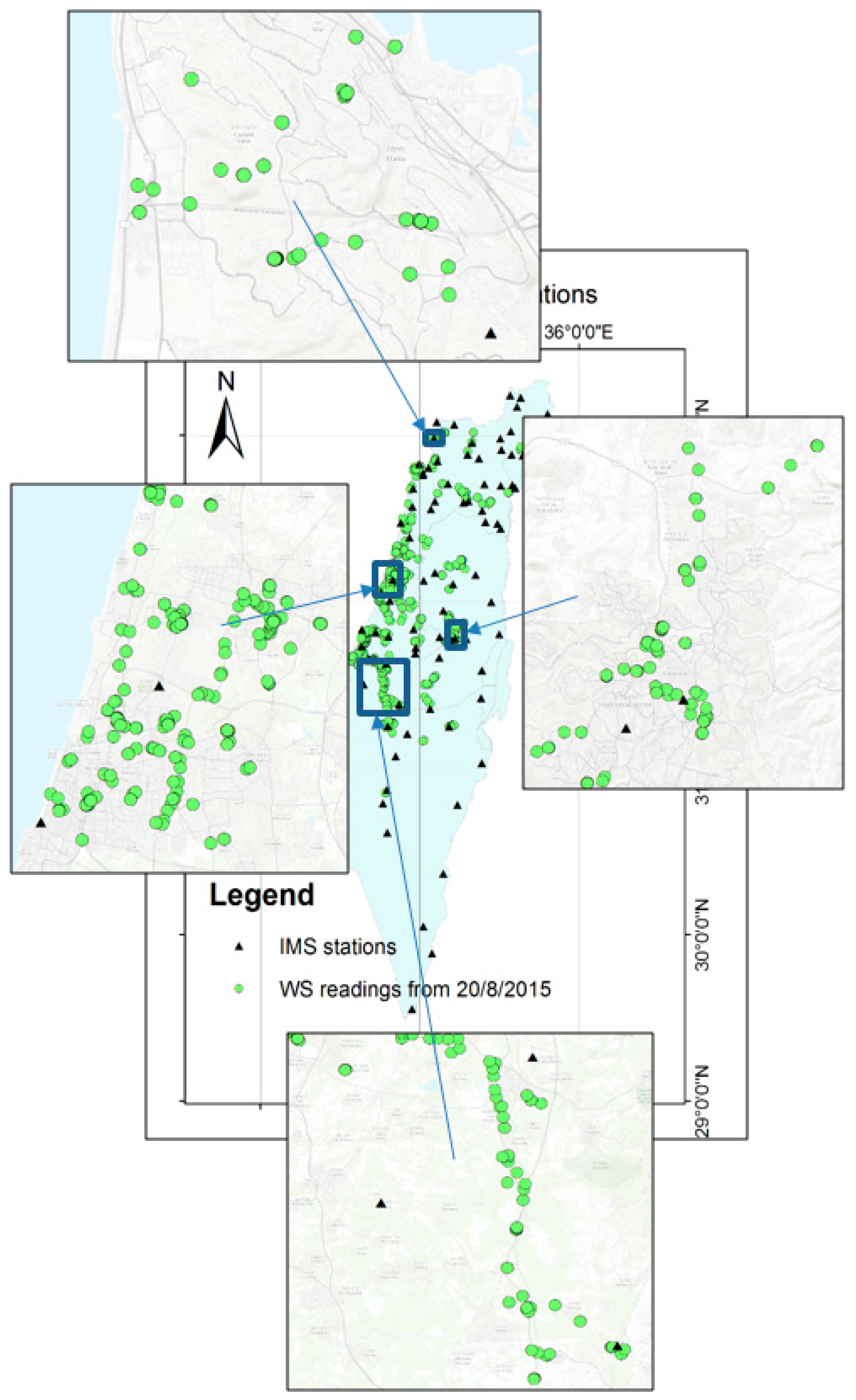
2 per single weather station, can benefit greatly. To demonstrate our methodology, we will evaluate and validate the empirical results in respect to fire weather parameters, used for simulation and assessment of the geosensor weather network of Israel. The presentation of our methodology and experimental results are made, proving the effectiveness of the developed and implemented algorithms, and the potential of the proposed augmentation and densification process.

2. Related Research

It is widely acknowledged that real-time geospatial data provide the best early warning source of information on damage and disaster management ([5]). Recent studies have already proven that the public is collaborating in sharing and collecting information (e.g., [6,7]), whereas in cases of emergencies and disasters, the public’s motivation for data collection is even bigger (e.g., [8,9]). Implementing crowdsourcing working schemes, supported by physical modern and reliable sensors that are carried by citizens, user-generated data enables to reduce the dependency on experts while using the fact that data can be collected or produced via diverse sources. The contribution of VGI for disaster situations in particular is implemented to some extent in various applications (e.g., [10,11]), where the latter showed that 26% of these applications are related to wildfire disaster management.
Weather and metrological data and information can be obtained nowadays from various non-authoritative sources originating in citizens and communities (e.g., [12,13]). Aggregating these data via the use of crowdsourcing techniques play a vital role in collecting and assessing reliable data in real time, especially in densely populated areas or regions having sparse meteorological networks ([14]). Since predictions assert that extreme weather events are expected to increase in frequency, duration and magnitude (e.g., [15,16]), dense, high-resolution and real-time observations will be increasingly required to observe metrological conditions and weather phenomena required for immediate detection and assessment.
Various examples that make use of public crowdsourcing collecting weather data (Citizen Science) exist. For example, the Community Collaborative Rain, Hail and Snow Network (CoCoRaHS) relies on a network of volunteers who measure and map precipitation to provide data for research, natural resource and education applications (e.g., [17,18]). The “Precipitation Identification Near the Ground” (PING) project, maintained by National Oceanic and Atmospheric Administration (NOAA), is another example, where volunteers issue reports on the type of precipitation that is occurring in real time ([19]). Still, in the majority of such projects, public crowdsourcing involves the use of low-cost and amateur-level sensors deployed and handled by citizens, and not the passive and active use of mobile devices equipped with sensors. Since today the number of embedded sensors in mobile devices is increasing, data collected can be crowdsourced to serve as input for various applications and services, for example OpenSignal and PressureNet (e.g., [20,21,22]). Still, physical weather variables can vary over small distances and with changing topographies, such that the reliability of these sensors in accurately capturing environmental conditions is still being investigated.
According to [23], densification of static geosensor network can be achieved by two means: (1) using hardware devices, hence deploying more sensors (“Hard” densification); or (2) using software solutions without additional hardware (“Soft” densification). One can consider the densification of an ESN as the densification of a geodetic control network, using different statistical methods ([24]). As in the case of multi-sensor data fusion methods, these are derived from statistics and are probabilistic methods ([25]), such as Bayesian fusion, Extended and Unscented Kalman-Filter, Grid-based, and Monte-Carlo-based. The main disadvantage of fusion based on probability methods is the inability to assess unknown conditions, hence relatively less appropriate for disaster management and assessment situations, which can be characterized by environmental condition anomalies.
Fusion and densification of data from physical geosensors with data collected using crowdsourcing is an innovative perception (e.g., [25,26]). Related research in this field primarily focuses on improving the coverage of physical geosensors—without using crowdsourced data. The problem of fusing data from fixed physical sensors with human (user-generated) sensors for the task of data quality improvement (to improve decision making) is referred to as Symbiotic Data Fusion and Processing problem (SDFP) [1]. Authors established a crowdsourcing support system for disaster surveillance, suggesting Centralized Decision Fusion (CDF) procedure for the platform, based on stochastic detection and estimation theory expressed in terms of binary hypothesis tests, using both value fusion and decision fusion. Another example is Social Fusion ([27]), a platform for fusing data from different sources and types (e.g., mobile data sensors, social networks and static networks sensors), with the objective to create context-aware applications. Fusion is done using a set of classifiers to extract meaningful contextual inferences from the data, while dividing the data collection mechanism from the classification phase.

3. Methodology

3.1. Introduction

Since weather data are an important factor for various manmade and natural environmental disaster management systems, fire weather parameters are chosen as case study. Fire weather is the meteorological data influencing on wild land fires ([28]). Two of the main fire weather parameters are: Ambient Temperature (AT) and Relative Humidity (RH) ([29]). Commonly used fire danger rating systems are the Canadian Forest Fire Danger Rating System (CFFDRS) and The National Fire Danger Rating System (NFDRS) used in the United States. Both system’s input requirements for AT and RH are depicted in Table 1.

3.2. Collected Data

Weather data collected in field experiments are AT and RH, together with auxiliary data, describing the environmental conditions existing during measurements, whereas some might affect the collection device, and thus the reliability and accuracy of the sensory weather data collected. The auxiliary data are: (1) Illumination, which might bias the weather data due to sun radiation that heats the collection platform (device); (2) Proximity, the detection of possible close range exterior disturbances; (3) Battery properties, which might affect the sensor readings, helping in understanding the current usage of the collection device; and (4) GPS, acquiring the measurements’ geographic position.

3.3. Data Collection Platform

Due to the use of crowdsourcing user-generated data collection methodology, which relies on random heterogeneous individuals situated near the interest area, it is required to use a portable device having the ability to collect the aforementioned weather and auxiliary data, and communicate it (via the Internet) to a central system. More common and widespread data collection platforms increase the probability of citizen participation in gathering data, increasing data volume, and presumably the overall network accuracy, density and reliability. Market examination showed that the Samsung Galaxy S4 (SG4) model GT-I9500, containing all the sensors necessary to deliver the aforementioned data, is widely used by citizens, with Samsung market share that is 25% ([32]). The SG4 contains GPS, geomagnetic positioning, as well as a gyrometer, accelerometer, barometer, thermometer, hygrometer, RGB light sensor, gesture sensor, proximity sensor and microphone ([33]).
The AT and RH sensor embedded in the SG4 device is SHTC1, manufactured by “Sensirion”, calibrated in a controlled environment. The official accuracy of the sensor is depicted in Table 2, where compared to the requirements of NFDRS and CFFDRS (Table 1), it is theoretically acceptable and well in the range. Theoretically, in normal conditions, the SHTC1 sensor has the potential to deliver with reliable readings, satisfying the purpose of our study ([34]).

3.4. Data Collection Application

Examining available apps suitable for the collection platform of weather data (android operating system), the application found to satisfy our requirements (variety of the recorded parameters, automation, user interface simplicity) was WeatherSignal, depicted in Figure 1. The app creates a crowdsourced based weather map, where users can collect a variety of weather data from the sensors embedded in their mobile devices.

3.5. Reference Data

Data from the Israel Meteorological Station (IMS) weather stations are used as reference, which comply with the World Meteorological Organization (WMO) standards ([36]). Table 3 depicts the accuracy of the AT and RH sensors used in the IMS meteorological stations. As of March 2016, there exist 84 unmanned stations for the area of Israel, whereas collected data and metadata are accessible to the public (www.data.gov.il).

3.6. Field Data Collection

The aim of the data collection scenarios is to provide analytical and statistical understandings of the collected weather data in terms of accuracy and reliability, required for the development of optimal and robust collection and processing methods and algorithms. This is done by collecting user-generated weather and auxiliary data in three different scenarios.

3.6.1. Scenario 1: Long-Duration Measurement

This scenario is aimed at verifying the measurements’ accuracies in non-laboratory conditions in respect to the official manufacturer accuracies (Table 2). Data were collected continuously for a long duration (12 h), while the SG4 was positioned statically in a shadowed place (serving as a meteorological hut) to eliminate heating from exposure to direct sunlight. The SG4 was located nearby an IMS station (Haifa Refineries, northern Israel) for measurements comparison, depicted in Figure 2. Sampling rate of measurements was every 10 s. Since data accuracy is determined in respect to IMS, in which measurements are averaged for every 10 min, the collected data were similarly averaged. Although the distance between locations is several kilometers, it is assumed that measurement values should be similar, mainly for such long duration and averaging of measurements.

3.6.2. Scenario 2: Short-Duration Measurements

This scenario is aimed at imitating an actual crowdsourcing collection process. The collection process does not enable to detect and eliminate outliers due to the small sample size, therefore post-processing is not practical. This scenario is composed of four different measurement sessions, each characterized by different measurement times, covering different environmental conditions throughout the day: 01:00–02:00, 08:00–09:00, 13:00–14:00 and 19:00–20:00. Measurements were carried out near two reference IMS stations (Haifa Refineries and Haifa University, depicted in Figure 2).

3.6.3. Scenario 3: Environmental Conditions Affect

SG4 readings might be biased by environmental conditions, mainly exposure to direct sunlight, which affect and bias the sensor readings. The aim here is to develop an algorithm, which can automatically detect and indicate when measurements are reliable (not biased by external influences). This is achieved by using different measurement scenarios, in which the SG4 was exposed to direct sunlight, biasing readings, and moved to a shaded place. The raw data collected during this scenario are analyzed for finding indicators, used in an algorithm that is aimed at identifying when the mobile sensor readings are stabilized, and thus can be used in real-time.

3.7. Data Analysis

Data analysis is aimed at determining the statistical characteristics of the collected data. The accuracy of the data is calculated using RMSE (Root Mean Square Error), depicted in Equation (1). This is similar to assessing the accuracy between datasets in geostatistical applications: using the measured user-generated weather data values (L), and the reference values measured by the official IMS stations (µ). If the parameter estimated using RMSE is unbiased, then the RMSE value equals the Standard Deviation (SD) value (σ).
R M S E =   i = 1 n ( L i   µ i ) 2 n
To quantify the uncertainty of a specific point estimates, in this case the uncertainty of the mean residuals, a confidence interval around the point estimates is calculated. Confidence interval that is based on the mean value might not be precise if the distribution of the data is not normal. If the residuals are normally distributed, than the RMSE value is multiplied by a value that represents the standard normal distribution probability factor error of the mean at 95% confidence level, Z = 1.96. Thus, the confidence interval is derived from the estimator/sample mean X ¯ as ( X ¯ Z * R M S E ,   X ¯ + Z * R M S E ) (e.g., [38]). Outlier elimination is done using the IQR (Inter-Quartile Range) method ([39]), whereas accepted data are considered to be in the interval of (1st quartile − 1.5 IQR, 3rd quartile + 1.5 IQR); this way, outliers can be detected and filtered for improving the results’ accuracy.
For the assessment of normal distribution (of residuals), the Shapiro–Wilk normality null-hypothesis test W is implemented ([40,41]), according to Equation (2). x(i) is the ith order statistic, x ¯ is the sample mean, and ai are constants derived from expected values of the order statistics sampled from the standard normal distribution and the covariance matrix. In case the significance parameter is less than the chosen alpha level (e.g., 0.05 for 5%), then the null hypothesis is rejected, meaning data are not normally distributed. The advantage of this test is that its result is objective, i.e., not interpreted (maybe subjectively) by the observer.
W = ( i = 1 n a i x ( i ) ) 2 i = 1 n ( x i x ¯ ) 2
Since both AT and RH measurements might present strong correlation, the Pearson correlation test ([42]) was conducted, according to Equation (3). This is done to identify whether sensor readings are biased. r is the Pearson correlation coefficient, X ¯ and Y ¯ are the sample mean of the first and second datasets, and X i and Y i are the value number i of the first and second datasets.
r = ( X i X ¯ ) ( Y i Y ¯ ) [ ( X i X ¯ ) 2 ( Y i Y ¯ ) 2 ] 1 2

3.8. Data Validation

Data validation is aimed at developing an algorithm for indicating whether the collected user-generated data are reliable to use; data measured in scenario 3 are used. The algorithm is based only on the collected data, not relying on any external (reference) data; results are later compared to IMS reference data for statistical analysis and verification. This algorithm uses data indicators (thresholds) that categorize the stabilization point: identifying, in real-time, when the collected weather data are reliable to use. Since sensors’ calibration times (needed for obtaining reliable results) are not constant and cannot be predetermined, we have classified a set of four parameters calculated dynamically (in real-time) during measurements: (1) Gradient value; (2) SD value; (3) Number of observations; and (4) Illumination reading. These parameters are chosen since when combined they serve as reliable indices to data measurements stabilization and continuity. The stabilization algorithm workflow is depicted in Figure 3.
Figure 4 depicts AT readings change due to exposure to direct sunlight (55,000 lux). When the collection device was moved to the shade, the light sensor measured few hundred lux only; only few minutes later the AT is stabilized to 21 °C, similar to the IMS reference data (RH readings have similar effect). This implies that although illumination value gives a good indication, only a combination of the four above-mentioned parameters can determine data stability. The four parameters, depicted in Table 4, were calculated empirically based on an optimization process using the five observations sessions in scenario 3.

3.9. Network Densification

Examining the potential of using user-generated weather data on a larger scale, we use the weather data from WeatherSignal’s crowdsourced weather map (www.weathersignal.com). WeatherSignal uses embedded mobile phone sensors to measure local atmospheric conditions, which are then displayed on their online weather map. WeatherSignal is used by hundreds of thousands of users worldwide, storing millions of user-generated weather data measurements. Such that by using the data stored in WeatherSignal’s database, we are practically using data from people who actively participate and continuously collect weather data.
Downloaded raw data have millions of data inputs, thus data filtering is necessary for eliminating irrelevant or erroneous readings. For this, an algorithm is developed, implemented in ArcMap using model-builder, depicted in Figure 5. The algorithm is composed from various queries executed in Python, depicted in Table 5, among others: geospatial boundaries of the desirable perimeter, sufficient location accuracy, and auxiliary sensory data thresholds. The filtering algorithm also aims to detect if the readings are taken indoor or outdoor by a supplementary set of queries, and also filter irrelevant or erroneous readings. Indoor AT maybe different from outdoor AT, such that filtering indoor observations is important. This was handled by three queries (see Table 5): (a) collection device is plugged to an external device (including portable power banks); (b) device is being charged; and (c) device is moving fast, i.e., in a car. In our dataset, for example, approximately 30% of all readings were filtered based on the use of these queries and thresholds. Alternatively, the use of map matching of collection devices’ positions with GIS layers (e.g., buildings, city boundaries, and roads) or Digital Surface Models of the area might be helpful. Still, accuracy of devices might be poor (bad GPS signal, multipath in built-up areas or position based on cellular network), such that matching might produce wrong results, or urban areas might be filtered out completely. To resolve this, we have applied a set of complementary statistical hypothesis tests (see Section 3.10) for identifying and removing data errors and outliers that might result from indoor readings.

3.10. Geo-Statistical Analysis

Two geo-statistical hypothesis tests are conducted on the WeatherSignal data after filtering, aimed at proving if it can be considered as an integral part of the IMS geosensor weather network. First, a local spatial auto-correlation null-hypothesis test, the Anselin Local Moran’s I ([43]), examining the spatial correlation of all readings to their vicinity. In case no outliers are detected, WeatherSignal data are statistically considered as an integral of the IMS network in terms of correlation. Rejecting the null-hypothesis means the differences between the values are not random, but are derived from non-compatible data—an outlier. Anselin Local Moran’s I statistic ( I i ) is depicted in Equation (4), where x i is the attribute for feature i (AT or RH), x ¯ is the mean of corresponding attribute, and w i , j is the spatial weight (distance) between feature i and j.
I i =   x i   X ¯ S i 2 · j = 1 ; j i n w i , j ( x j X ¯ ) S i 2 =   j = 1 ; j i n ( x j X ¯ ) 2 n 1   Z I i =   I i E [ I i ] V [ I i ] E   [ I i ] =     j = 1 ; j i n w i , j n 1 V   [ I i ] = E [ I i 2 ] E [ I i ] 2
Second, a global spatial auto-correlation null-hypothesis test, the Anselin Global Moran’s I ([44]), examining the spatial correlation of the features location with respect to specific feature value. This test is global, meaning it checks the complete spatial pattern of all data (clustered, dispersed or random). If the null hypothesis is rejected, then the data are not randomly spread, while if the result is significant enough, it can be stated that data are clustered, meaning WeatherSignal data are an integral complementary part of the IMS geosensor weather network. Anselin Global Moran’s I statistic (I) is depicted in Equation (5), where z i is the deviation of feature i (AT and RH) from its mean, S 0 is the aggregation of spatial weights, and w i , j is the spatial weight (distance) between feature i and j.
I =   n S 0 · i = 1 n j = 1 n w i , j z i z j i = 1 n z i 2 S 0 =   i = 1 n j = 1 n w i , j   Z I =   I E [ I ] V [ I ] E   [ I ] =   1 / ( n 1 ) V   [ I ] = E [ I 2 ] E [ I ] 2

4. Experimental Results

4.1. Scenario 1

Total number of measurements cumulates to 1600, expressing average sampling rate of approximately 30 s, generating a total number of 73 analyzed sessions (the numbers are different from the planned 10 s interval of this experiment since some epochs were missing or showed irrelevant measurements).

4.1.1. Ambient Temperature Results

The AT mean difference between the SG4 and the IMS measurements is 1.2 °C, with SD of 2 °C and RMSE of 2.3 °C. The estimation interval of the mean with probability of 95% is 1.2 °C ± 4.5 °C, with minimum and maximum difference values of −1.9 °C and 9.2 °C, respectively. Results might include gross errors, which will be checked later. Seventy-two percent of calculated residuals of measured value are higher than the reference value, indicating that the SG4 tends to overestimate the AT. That explains also the high positive residual values in contrary to the small negative residual values.
Due to the relatively large sample size (73 measurements), it is assumed that the residuals are derived from a normal distribution. To verify this, a combination of visual analysis with statistical test is conducted. The result of the Shapiro–Wilk test is shown in Table 6 (top). The significance level of 0.01 (<0.05) implies that the null hypothesis is rejected; therefore, the population is not normally distributed. An examination of the histogram and normal probability plot showed that except few suspicious measurements the data can be considered as normally distributed, thus a conclusion regarding the distribution of the data is ambiguous. Accordingly, outlier detection is performed to identify observations with erroneous values using boxplot visualization, found useful for comparing distributions and identifying outliers. Boxplot is less sensitive to extreme values of data since not using mean or SD but quartiles instead, not limited to normal distribution ([40]). Consequently, several readings are identified as outliers outside the boxplot whisker. Removing these outlier readings, the AT is analyzed again, with results showing reduced statistics values: estimation interval of 95% is 0.9 °C ± 3.2 °C, RMSE of 1.6 °C and minimum and maximum difference values of −1.9 °C and 3.9 °C, respectively. Executing the Shapiro–Wilk normality test again, depicted in Table 6 (bottom), results ratify the assumption that the data are derived from a normal distributed population (Sig. 0.4 > 0.05 Alpha), also verified by a boxplot visualization of data.

4.1.2. Relative Humidity Results

Results of scenario 1 RH measurements produced a mean difference between the SG4 and the reference IMS measurements of −2%, with SD and RMSE values of 8%. Assuming the data are normally distributed, the estimation interval of 95% is −2% ± 16%, and minimum and maximum difference values of −21% and 15%, respectively. Unlike AT, data here are normally distributed, proved by the Shapiro–Wilk normality test (Sig. 0.1 > 0.05 alpha), depicted in Table 7, as well as the boxplot visualization, having no data outliers.

4.1.3. Correlation between Relative Humidity and Ambient Temperature

When both SG4 AT and RH measurements were compared with the reference IMS data, there existed a strong correlation between measurements: whenever the AT measurement is higher than the reference (“true”) value, the RH measurement is lower than the reference value. Figure 6 compares both residual values. The Pearson correlation test results are depicted in Table 8, indicating that when the AT residuals are strong positive, the RH residuals will be strong negative, and vice versa, proving that there is a strong negative correlation. Such that whenever a parameter is biased, it is affecting the other parameter, implying that the sensor is biased. This can be explained by several assumptions, the main one is that due to the fact that the same sensor is used simultaneously for measuring AT and RH, it affects (biasing) all the measured parameters. Another assumption is that existing environmental conditions affect the sensor readings, thus bias them for both parameters.

4.1.4. Summary and Conclusions

Analyses indicate that both AT and RH measurements are normally distributed, although discrepancies between the declared SHTC1 values and the actual field sessions’ values are fairly big. A comparison of accuracy requirements and accuracy results of different sessions is presented in Table 9, showing that the user-generated weather data are in the locale of both CFFDRS and NFDRS requirements.

4.2. Scenario 2

A comparison of statistics of scenario 2 and scenario 1, depicted in Table 10, shows an improvement, to some extent. For example, the mean residual, RMSE, SD and the maximum residual range of the AT measurements were reduced by close to 50%. Possible explanation for these might be due to existing environmental conditions in the measurement perimeter, which caused the mobile sensor to heat and bias the measurements during the long duration scenario 1. In the short-duration measurements (scenario 2), due to short collection times, the sun position remained similar, so the collection device was shaded during the whole measurement phase. Another explanation can be due to drifting of the SHTC1 sensor, which although considered negligible according to SHTC1’s datasheet, has an effect on the measurements (similarly to the actual evaluated accuracy that was worse than the official one). When compared to the fire danger rating systems (Table 9), it appears as if the user-generated AT accuracy is similar to the NFDRS requirement, concluding that measurements can be considered as input for such application. The user-generated RH accuracy is closer to the CFFDRS requirement, still biased in 2% than needed. Overall, results of both scenario 1 and scenario 2 experiments prove that the proposed methodology of using user-generated weather data for augmentation of weather geosensor network can be considered, even when no data post-processing is made.

4.3. Scenario 3

A series of five sessions were conducted, depicted in Table 11, used as input for the stabilization process. Figure 7 shows the gradient parameter of the AT measurements calculated for different number of readings, to determine the necessary number of readings for an unambiguous detection of the stabilization point. It can be inferred that only after 30 readings stabilization is accomplished, filtering gradient calculated on similar AT values (near zero gradient value). Accordingly, the threshold of the gradient is chosen to be less than 0.05. SD value, which is a measure of decline, can predict if measurements are scattered, or persistent, thus stabilization is achieved when measurement values are similar, without fluctuations. Similarly, to gradient, 30 readings presented an SD value having good data trend.
It was found that if illumination is less than 50,000 lux, it does not mean that data are stabilized, only that the collection device is not directly exposed to the sun. Only a combination of the four parameters’ thresholds can determine data stability. The four stabilization parameters were calculated empirically, analyzed in respect to the five sessions, whereas threshold value for each is defined in Table 4, with stabilization algorithm workflow depicted in Figure 3.
A comparison of the IMS AT data (reference) with user-generated readings together with the stabilization algorithm indicators is depicted in Figure 8. Stabilization point is determined automatically and correctly. Figure 8 shows the effect of lux values, proving that it takes some time for the measurements to stabilize and produce accurate readings. The AT (and also RH) readings from both data sources are similar after the stabilization (calibration) point is determined automatically.

5. Applicative Demonstration

5.1. Weather Data Collection

The potential of using crowdsourced weather data is illustrated by the use WeatherSignal’s crowdsourced weather map. Observations were downloaded from WeatherSignal database for the period of 1 June 2015 to 22 August 2015. More than two million records were retrieved, expressing approximately 24,000 readings per day, and 1000 readings per hour. Among others, every reading (record) includes: location, AT, RH, illumination, speed, and proximity measurements. Using a simple spatial query for the area of Israel, a total of 7600 readings for the epoch of 17 August 2015 to 20 August 2015 were downloaded, where 3755 readings were taken on 20 August 2015 alone. Figure 9 depicts areas where the density of the user-generated WeatherSignal weather data significantly contributes to the density of existing IMS weather stations. It is clear that the crowdsourced-based readings are filling gaps in areas having no coverage or sparse weather stations.

5.2. Pre-Processing of User-Generated Weather Data

Filtering process, depicted in Table 5, is implemented on the user-generated weather data of 20 August 2015, in which inaccurate GPS position (close to 1200 readings), data that are incomplete, e.g., missing AT, RH (327 readings), or not relevant, e.g., indoor (more than 1000 readings), are filtered and not used, resulting in 730 readings (out of the initial 3755). Since weather is constantly changing, we have focused on a specific time epoch, in which the densification process will be executed; the epoch of 10:00 to 12:00 was chosen, resulting in 57 readings.

5.3. Geo-Statistical Analysis

5.3.1. Local Spatial Auto-Correlation

Results of the hypothesis test for the RH data indicated that there exist three outliers, meaning measurements are incompatible with surrounding RH readings; all outliers are IMS measurements, with none that is user-generated. This implies that the hypothesis test theoretically confirms that the user-generated RH data downloaded from WeatherSignal can be considered as part of the comprehensive weather network. For the AT, the test detected five outliers, all with values significantly higher than their surroundings, again originating from IMS measurements, with none that is user-generated, concluding the same inference. Although results suggest that all outliers are IMS measurements, it should be stated that IMS readings are considered more reliable. Outliers can be caused due to the topography of the area, which was not considered here, where the only spatial relationship defined was distance. Moreover, all the readings (user-generated and IMS) were considered as equally-weighted, since the aim was to prove that both data sources are complementary. Therefore, it is possible that clusters of biased user-generated weather readings caused accurate IMS readings to be detected as outliers. This issue is depicted in Figure 10, visualizing both hypothesis test results, showing that in some cases, the closest readings to the detected IMS outliers are clustered user-generated readings.

5.3.2. Global Spatial Auto-Correlation

Results of this hypothesis test are detailed in Table 12, indicating that the null hypothesis (z-score) is rejected for both RH and AT measurements. The positive value for Moran’s index of both indicates that there exist spatial clusters of homogeneous data. The output z-score value for both (6.9 and 10.4, respectively) indicates that there exists less than 1% likelihood that the clustered patterns could be the result of random chance. Since data are not random, the user-generated weather data, along with the IMS weather data, can be considered as a unified dataset having spatial correlation.

5.4. Densification

Densification is implemented via Ordinary Kriging interpolation, considered as most appropriate for weather data (e.g., [45,46]), on both user-generated and IMS weather data. Ordinary Kriging has several semivariogram (spatial correlation) models that can be used, created based on the empirical data; the model that best fits the semivariogram is chosen here (e.g., curve should pass through the center of the cloud of binned values and as closely as possible to the averaged values). Models found as best fit for AT and RH semivariograms are spherical and exponential, respectively, depicted in Figure 11.
Interpolation of AT readings was implemented three times: on the WeatherSignal user-generated data, on the IMS data, and on both. Subtracting the IMS interpolation raster from the user-generated one, results varied from −2.7 °C to 1.2 °C, with an average value of −1.1 °C and SD of 1.2 °C. The absolute maximal differences values are in areas with scarce user-generated readings, implying interpolation that calculates values relying on incomplete data, i.e., insufficient user-generated weather data. Similar to AT, RH user-generated interpolation map was found to be less continuous than the IMS one, with interpolation that is less accurate in areas with sparse data, leading to bigger discrepancies. Subtracting both maps, difference values are in the range of −3.3% and 14.1%, with an average value of 6.7% and SD of 3.5%. The significant value differences are mainly in areas with fewer user-generated readings. Comparing areas having more user-generated readings, the difference in AT and RH values were less than −1 °C and less than 5%, respectively, which is a good result. Although differences exist, the overall results are satisfying considering they were obtained by users contributing voluntarily having no special equipment. This is in comparison to the IMS data, which is an official weather network, maintained, supervised and quality controlled. It is likely that the reason for the differences are mainly due to the interpolation, which decreased the accuracy of the data, mainly in areas having low density of user-generated data.
For densifying both datasets, two new weather maps were created using Ordinary Kriging interpolation, containing data from both sources. Interpolation results for AT and RH are depicted in Figure 12. Inspecting both maps, it is clear that they are continuous and similar in value, with no visible anomalies detected all over the analyzed area. This supports the premise that user-generated measurements are sound, not biasing the authoritative measurements, and can be considered for densification. More importantly, it is clear that some physical conditions are revealed and made clear on a localized level (mainly in the center area of Israel), which were hard to identify unless the user-generated data were used. Another interesting result is that the existing value levels for both interpolations correspond—to some extent—to the topography existing in Israel, and to the meteorological conditions, distributed from south to north. These are the direct result of using comprehensive observations, in this case user-generated and official weather measurements.

6. Conclusions and Future Work

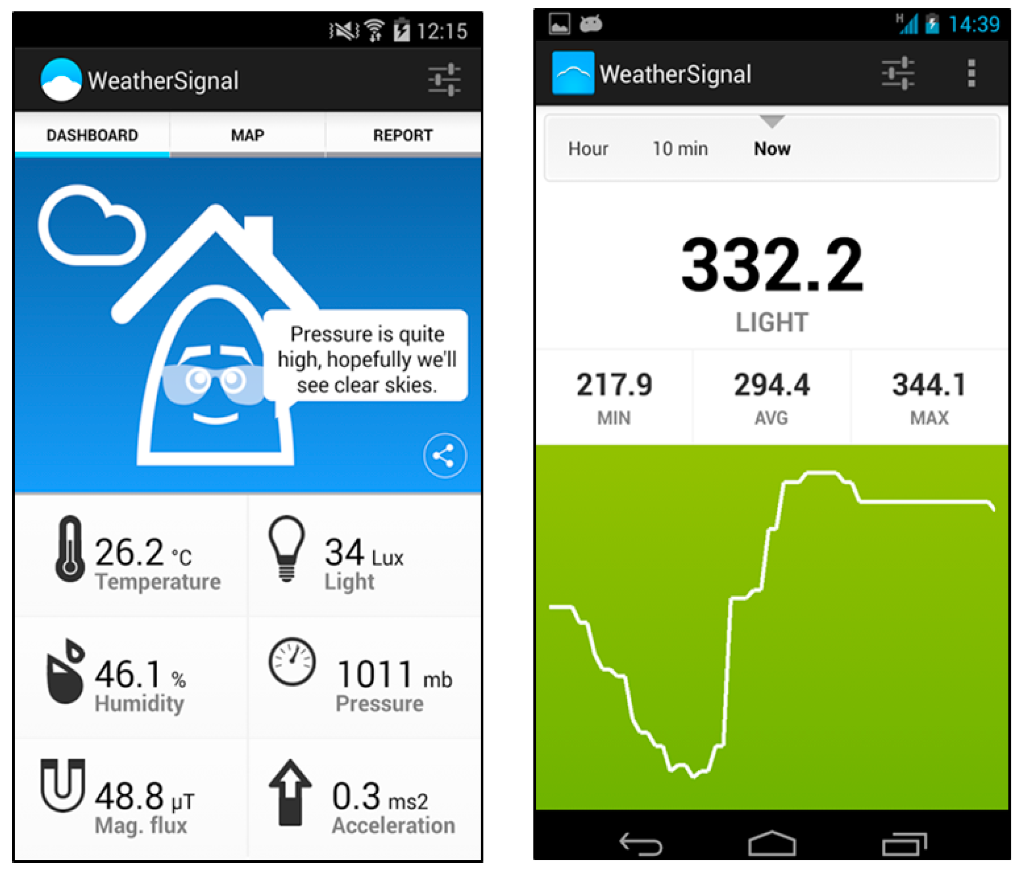
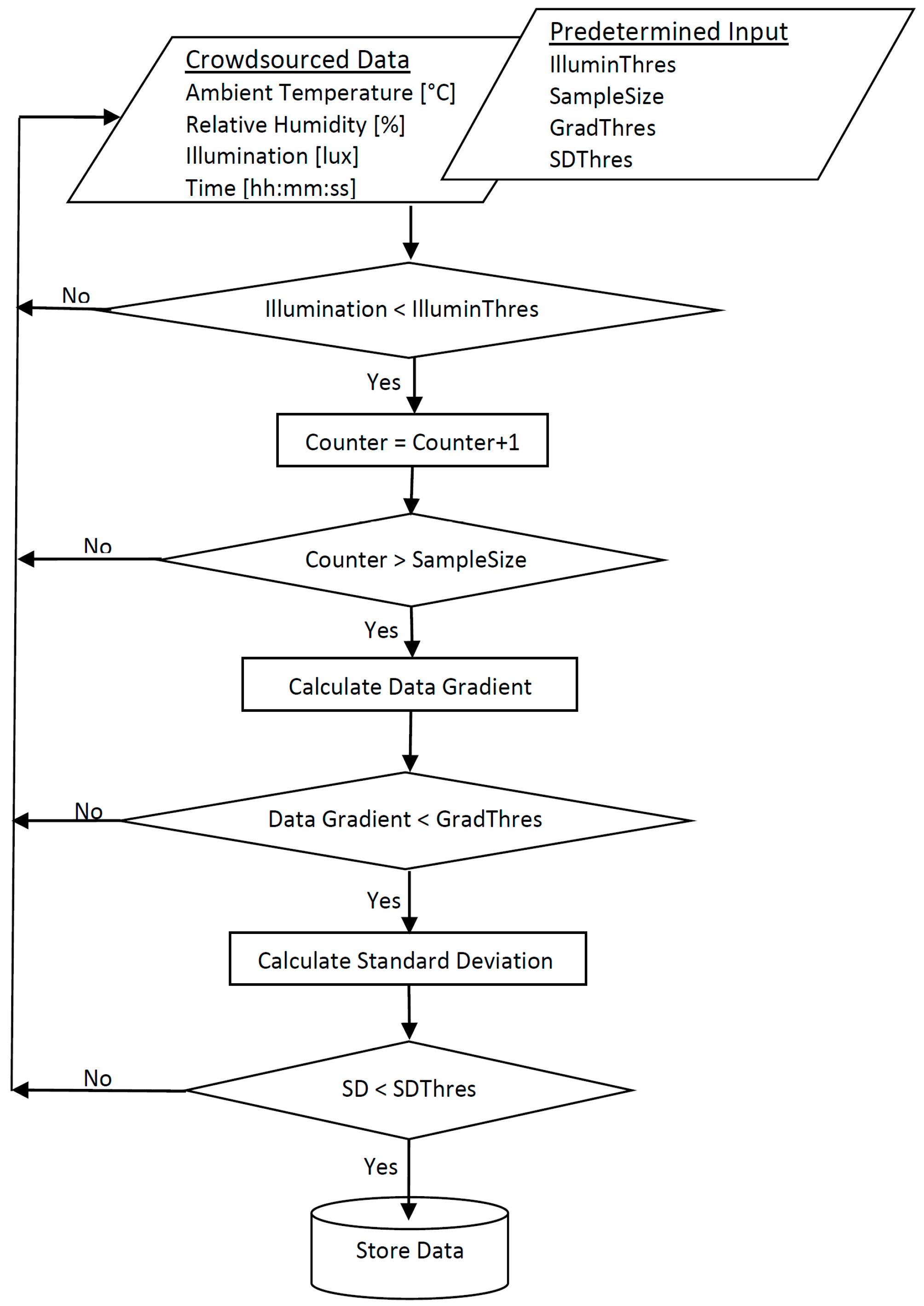
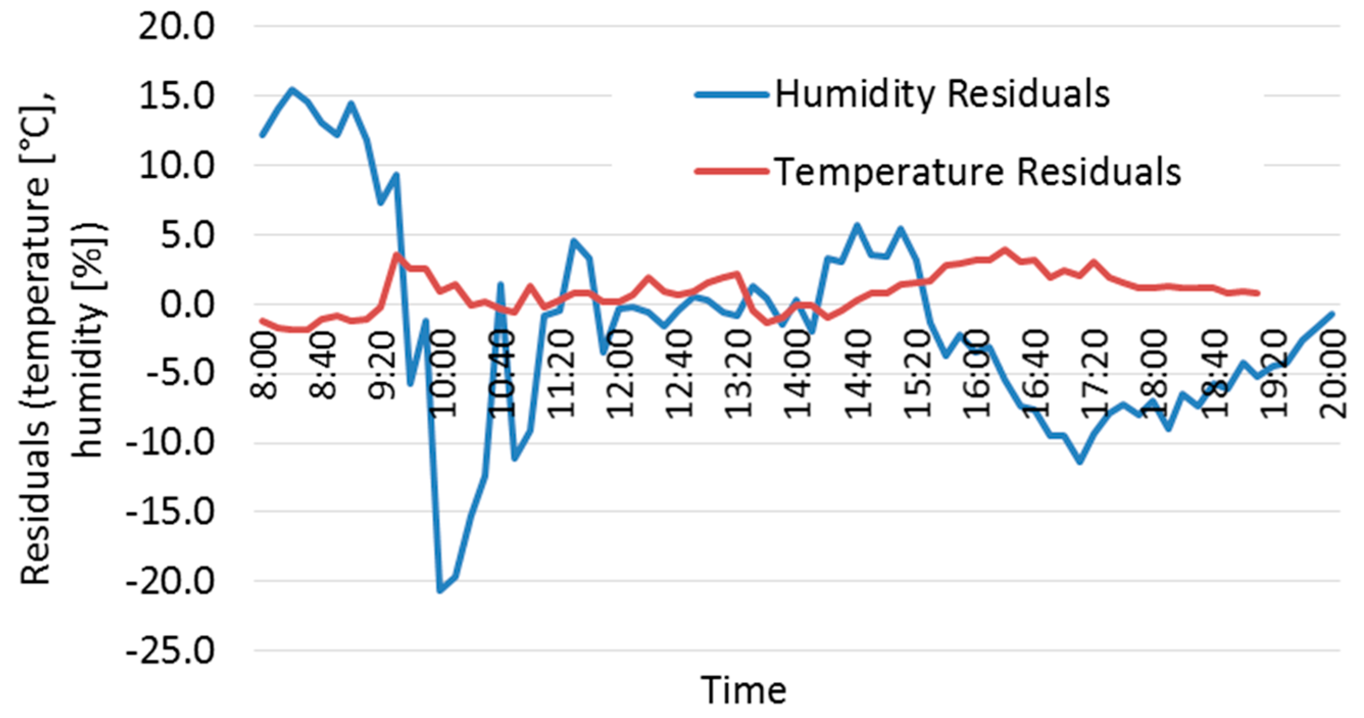
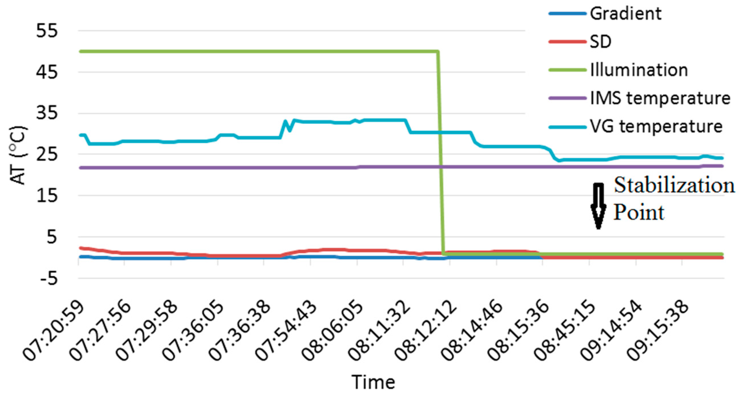
The conception of using crowdsourced user-generated weather sensor data from mobile devices for the augmentation of static geosensor weather networks was presented, accompanied by developed methodology and tailored functionalities. Experiments made with the SG4 smartphone showed that with accuracies obtained, collected data can be considered for a variety of applications. Certain issues and automatic procedures were addressed to guarantee the overall reliability, namely stabilization identification and geo-statistical analysis, enabling real-time data collection without the need of reference data. Research proved that with proper handling of data, the complementary crowdsourced user-generated data can be considered for the purpose of augmentation. Hypothesis tests statistically proved that user-generated weather data are considered as an integral part of the authoritative weather network, correlating to surroundings observations locally and globally.
Future work will investigate the use of larger volumes of data collected in field experiments and communication protocols of observations in real time, together with assessment of the user-generated data contribution on actual systems. Work on the densification process is planned, taking into account additional factors, such as observation weights, network structure, and existing topography. Other physical sensory data, such as pressure, will be investigated, whereas in Israel only 10 IMS stations are equipped with pressure sensors, such that user-generated data will have higher influence and contribution.
In conclusion, the results of this research are valuable and positive, showing that sensors embedded in modern mobile devices can be used to collect weather data via crowdsourcing process to augment static geosensor weather networks, providing more observations of weather parameters used for network densification. It is believed that countries and regions with sparse dispersion of static geosensor networks can benefit from these working methodologies, while in the future, together with technological and communication developments, real-time user-generated weather data will be considered as reliable as authoritative ESN.

Acknowledgments

The authors would like to thank IMS and KKL-JNF for delivering with information regarding the position and impact zones of IMS; and the OpenSignal team, delivering with valuable information and assistance regarding their web service and data.

Author Contributions

The methodology and algorithms were developed by Shay Sosko and Sagi Dalyot, with implementations, experiments and analyses carried out by Shay Sosko.

Conflicts of Interest

The authors declare no conflict of interest.

References

  1. Liu, J.W.S.; Chu, E.T.H.; Tsai, P.H. A Framework for Fusion of Symbiotic Human Sensor and Physical Sensor Data. Technical Report No. TR-IIS-12-007. 2012. Available online: http://www.iis.sinica.edu.tw/page/library/TechReport/tr2012/tr12007.pdf (accessed on 6 March 2016).
  2. Goodchild, M.F.; Glennon, J.A. Crowdsourcing Geographic Information for disaster response: A research frontier. Int. J. Digit. Earth 2010, 3, 231–241. [Google Scholar] [CrossRef]
  3. Estellés-Arolas, E.; González-Ladrón-de-Guevara, F. Towards an integrated crowdsourcing definition. J. Inf. Sci. 2012, 38, 189–200. [Google Scholar] [CrossRef]
  4. NOAA. The USHCN Version 2 Serial Monthly Datasets. 2012. Available online: https://www.ncdc.noaa.gov/oa/climate/research/ushcn/ (accessed on 15 May 2016). [Google Scholar]
  5. National Research Council. Improving Disaster Management: The Role of IT in Mitigation, Preparedness, Response, and Recovery. 2007. Available online: https://www.nap.edu/read/11824/chapter/3 (accessed on 20 May 2016).
  6. Coleman, D.J.; Georgiadou, Y.; Labonte, J. Volunteered geographic information: The nature and motivation of producers. Int. J. Spat. Data Infrastruct. Res. 2009, 4, 332–358. [Google Scholar]
  7. Hand, E. Citizen science: People power. Nature 2010, 466, 685–687. [Google Scholar] [CrossRef] [PubMed]
  8. Starbird, K. Digital volunteerism during disaster: Crowdsourcing information processing. In Proceedings of the Conference on Human Factors in Computing Systems, Vancouver, BC, Canada, 7–12 May 2011.
  9. Haworth, B.; Bruce, E. A review of Volunteered Geographic Information for disaster management. Geogr. Compass 2015, 9, 237–250. [Google Scholar] [CrossRef]
  10. Vivacqua, A.S.; Borges, M.R.S. Taking advantage of collective knowledge in emergency response systems. J. Netw. Comput. Appl. 2012, 35, 189–198. [Google Scholar] [CrossRef]
  11. Horita, F.E.A.; Degrossi, L.C.; Assis, L.F.F.G.; Zipf, A.; Porto de Albuquerque, J. The use of volunteered geographic information and crowdsourcing in disaster management: A systematic literature review. In Proceedings of the Nineteenth Americas Conference on Information Systems, Chicago, IL, USA, 15–17 August 2013.
  12. Wiggins, A.; Crowston, K. From conservation to crowdsourcing: A typology of citizen science. In Proceedings of the 2011 44th Hawaii International Conference on System Science (HICSS), Kauai, HI, USA, 4–7 January 2011.
  13. Evangelos, N.; Vourvopoulos, A.; Langheinrich, M.; Campos, P.; Doria, A. Atmos: A hybrid crowdsourcing approach to weather estimation. In Proceedings of the 2014 ACM International Joint Conference on Pervasive and Ubiquitous Computing: Adjunct Publication (UbiComp ’14 Adjunct), Seattle, WA, USA, 13–17 September 2014.
  14. GCOS. Implementation Plan for the Global Observing System for Climate in Support of the UNFCCC (2010 Update). GOOS-184, GTOS-76, WMO-TD/No. 1523. 2010. Available online: http://www.wmo.int/pages/prog/gcos/Publications/gcos-138.pdf (accessed on 20 October 2016).
  15. Intergovernmental Panel on Climate Change (IPCC). Summary for policymakers. In Managing the Risks of Extreme Events and Disasters to Advance Climate Change Adaptation; A Special Report of Working Groups I and II of the Intergovernmental Panel on Climate Change; Field, C.B., Barros, V., Stocker, T.F., Qin, D., Dokken, D.J., Ebi, K.L., Mastrandrea, M.D., Mach, K.J., Plattner, G.-K., Allen, S.K., et al., Eds.; Cambridge University Press: Cambridge, UK; New York, NY, USA, 2012; pp. 1–19. [Google Scholar]
  16. Muller, C.L.; Chapman, L.; Grimmond, C.S.B.; Young, D.T.; Cai, X. Sensors and the city: A review of urban meteorological networks. Int. J. Climatol. 2013, 33, 1585–1600. [Google Scholar] [CrossRef]
  17. Cifelli, R.; Doesken, N.; Kennedy, P.; Carey, L.D.; Rutledge, S.A.; Gimmestad, C.; Depue, T. The community collaborative rain, hail, and snow network: Informal education for scientists and citizens. Bull. Am. Meteorol. Soc. 2005, 86, 1069–1077. [Google Scholar] [CrossRef]
  18. Illingworth, S.M.; Muller, C.L.; Graves, R.; Chapman, L. UK citizen rainfall network: A pilot study. Weather 2014, 69, 203–207. [Google Scholar] [CrossRef]
  19. Elmore, K.L.; Flamig, Z.L.; Lakshmanan, V.; Kaney, B.T.; Farmer, V.; Reeves, H.D.; Rothfusz, L.P. mPING: Crowd-sourcing weather reports for research. Bull. Am. Meteorol. Soc. 2014, 95, 1335–1342. [Google Scholar] [CrossRef]
  20. Boulos, M.N.K.; Resch, B.; Crowley, D.N.; Breslin, J.G.; Sohn, G.; Burtner, R.; Pike, W.A.; Jezierski, E.; Chuang, K.-Y.S. Crowdsourcing, citizen sensing and sensor web technologies for public and environmental health surveillance and crisis management: Trends, OGC standards and application examples. Int. J. Health Geogr. 2011, 10, 67. [Google Scholar] [CrossRef] [PubMed]
  21. Overeem, A.; Robinson, J.C.R.; Leijnse, H.; Steeneveld, G.J.; Horn, B.K.P.; Uijlenhoet, R. Crowdsourcing urban air temperatures from smartphone battery temperatures. Geophys. Res. Lett. 2013, 40, 4081–4085. [Google Scholar] [CrossRef]
  22. Muller, C.L.; Chapman, L.; Johnston, S.; Kidd, C.; Illingworth, S.; Foody, G.; Overeem, A.; Leigh, R.R. Crowdsourcing for climate and atmospheric sciences: Current status and future potential. Int. J. Climatol. 2015, 35, 3185–3203. [Google Scholar] [CrossRef]
  23. Ge, L.; Rizos, C.; Han, S.; Zebker, H. Mining subsidence monitoring using the combined InSAR and GPS approach. In Proceedings of the 10th International Symposium on Deformation Measurements, Anaheim, CA, USA, 19–22 March 2001.
  24. Fok, H.S.; Baki, I.H.; Schaffrin, B. Comparison of four geodetic network densification solutions. Surv. Rev. 2009, 41, 44–56. [Google Scholar] [CrossRef]
  25. Khaleghi, B.; Khamis, A.; Karray, F.O.; Razavi, A.N. Multisensor data fusion: A review of the state-of-the-art. Inf. Fusion 2013, 14, 28–44. [Google Scholar] [CrossRef]
  26. Llinas, J.; McNeese, M.; Hall, D.L. Modeling and Mapping of Human Source Data. Pennsylvania State Univ University Park Office of Sponsored Programms, 2011. Available online: https://ntrl.ntis.gov/NTRL/dashboard/searchResults/titleDetail/ADA546038.xhtml (accessed on 20 February 2017). [Google Scholar]
  27. Beach, A.; Gartrell, M.; Xing, X.; Han, R. Fusing mobile, sensor, and social data to fully enable context-aware computing. In Proceedings of the Eleventh Workshop on Mobile Computing Systems & Applications, Annapolis, MD, USA, 22–23 February 2010.
  28. Schroeder, M.J.; Buck, C.C. Fire Weather: A Guide for Application of Meteorological Information to Forest Fire Control Operations. Available online: http://digitalcommons.usu.edu/barkbeetles/14/ (accessed on 20 February 2017).
  29. Collaud, C.M.; Andrews, E.; Asmi, A.; Baltensperger, U.; Bukowiecki, N.; Day, D.; Fiebig, M.; Fjaeraa, A.M.; Flentje, H.; Hyvarinen, A.; et al. Aerosol decadal trends—Part 1: In-situ optical measurements at GAW and IMPROVE stations. Atmos. Chem. Phys. 2013, 13, 869–894. [Google Scholar] [CrossRef] [Green Version]
  30. Lawson, B.D.; Armitage, O.B. Weather Guide for the Canadian System of Forest Fire Danger Rating; Northern Forestry Centre: Edmonton, AB, Canada, 2008.
  31. National Wildfire Coordinating Group. Interagency Wildland Fire Weather Station Standards & Guidelines. Available online: https://www.nwcg.gov/sites/default/files/products/pms426-3.pdf (accessed on 10 August 2016).
  32. International Data Corporation. Smartphone OS Market Share, 2016 Q2. Available online: http://www.idc.com/prodserv/smartphone-os-market-share.jsp (accessed on 10 August 2016).
  33. Nickinson, P. Samsung Galaxy S4 Specs. 2013. Available online: http://www.androidcentral.com/samsung-galaxy-s4-specs (accessed on 20 August 2016).
  34. Sensirion. Data Sheet SHTC1 Humidity and Temperature Sensor IC for High-Volume Applications. 2013. Available online: http://www.sensirion.com/fileadmin/user_upload/customers/sensirion/Dokumente/Humidity/Sensirion_Humidity_SHTC1_Datasheet_V3.pdf (accessed on 5 March 2016).
  35. OpenSignal. Sensing Samsung: The Evolution of Sensors in the Galaxy S Series. 2015. Available online: http://opensignal.com/blog/category/weathersignal-2/ (accessed on 10 January 2016).
  36. World Meteorological Organization. Guide to Meteorological Instruments and Methods of Observation. WMO-No. 8. 2008. Available online: https://www.wmo.int/pages/prog/gcos/documents/gruanmanuals/CIMO/CIMO_Guide-7th_Edition-2008.pdf (accessed on 20 May 2016).
  37. Israel Meteorological Station. Israel Meteorological Service User Guide for Using Meteorological Data. 2015. Available online: http://www.ims.gov.il/IMSEng/CLIMATE (accessed on 10 August 2016). [Google Scholar]
  38. Drummond, J.E. Elements of Spatial Data Quality; Guptill, S.C., Morisson, J.L., Eds.; Pergamon: Oxford, UK, 1995. [Google Scholar]
  39. Seo, S.; Marsh, G.M. A Review and Comparison of Methods for Detecting Outliersin Univariate Data Sets; Department of Biostatistics, Graduate School of Public Health: Seattle, WA, USA, 2006. [Google Scholar]
  40. Natrella, M.; Croarkin, C.; Tobias, P.; Filliben, J.J. NIST/SEMATECH E-Handbook of Statistical Methods; National Institute of Standards and Technology: Gaithersburg, MD, USA, 2012.
  41. Shapiro, S.S.; Wilk, M.B.; Chen, H.J. A comparative study of various tests for normality. J. Am. Stat. Assoc. 1968, 63, 1343–1372. [Google Scholar] [CrossRef]
  42. Rodgers, J.L.; Nicewander, W.A. Thirteen ways to look at the correlation coefficient. Am. Stat. 1988, 42, 59–66. [Google Scholar] [CrossRef]
  43. Anselin, L. Local indicators of spatial association-LISA. Geogr. Anal. 1995, 27, 93–115. [Google Scholar] [CrossRef]
  44. Anselin, L.; Ibnu, S.; Youngihn, K. GeoDa: An introduction to spatial data analysis. Geogr. Anal. 2006, 38, 5–22. [Google Scholar] [CrossRef]
  45. Eldrandaly, K.A.; Abu-Zaid, M.S. Comparison of six GIS-based spatial interpolation methods for estimating airtemperature in Western Saudi Arabia. J. Environ. Inform. 2011, 18, 38–45. [Google Scholar] [CrossRef]
  46. Hofstra, N.; Haylock, M.; New, M.; Jones, P.; Frei, C. Comparison of six methods for the interpolation of daily european climate data. J. Geophys. Res. Atmos. 2008. [Google Scholar] [CrossRef]
Figure 1. WeatherSignal application dashboard (source: [35]).
Ijgi 06 00061 g001
Figure 2. Scenarios 1 and 2: SG4 locations (green triangle) with reference IMS locations (marked with circled X).
Ijgi 06 00061 g002
Figure 3. Stabilization algorithm workflow.
Ijgi 06 00061 g003
Figure 4. Ambient Temperature stabilization time: readings change due to direct sunlight exposure, although illumination readings are not sufficient in indicating measurement stability.
Ijgi 06 00061 g004
Figure 5. WeatherSignal data filtering algorithm (ArcGIS 10.2 model builder).
Ijgi 06 00061 g005
Figure 6. Comparison of Ambient Temperature and Relative Humidity residuals.
Ijgi 06 00061 g006
Figure 7. Gradient (C°/number of observation) of Ambient Temperature measurements for different moving average calculations.
Ijgi 06 00061 g007
Figure 8. Comparison between the automatic stabilization algorithm results on user-generated Ambient Temperature measurements (denoted as VG, cyan) and reference IMS data (purple).
Ijgi 06 00061 g008
Figure 9. Areas with high density of user-generated WeatherSignal (denoted as WS) data for 20 August 2015 (green circles) in respect to IMS stations (black triangles).
Ijgi 06 00061 g009
Figure 10. Outlier analysis results of Anselin Local Moran’s I for: (a) Relative Humidity; and (b) Ambient Temperature.
Ijgi 06 00061 g010
Figure 11. Semivariogram analysis for: (a) Ambient Temperature; and (b) Relative Humidity measurements. Blue lines represent the spherical (a) and exponential (b) models. Blue crosses, averaged values; red points, user-generated readings; green lines, local polynomials.
Ijgi 06 00061 g011
Figure 12. Ordinary Kriging interpolation of user-generated and IMS measurements: (a) Ambient Temperature; and (b) Relative Humidity.
Ijgi 06 00061 g012
Table 1. Comparison between fire weather parameters of CFFDRS and NFDRS (source: [30,31]).
ParameterCFFDRSNFDRS
Ambient Temperature (AT) accuracy (°C)0.51
Ambient Temperature (AT) resolution (°C)0.10.6
Relative Humidity (RH) accuracy (%)52
Relative Humidity (RH) resolution (%)11
Table 2. SHTC1 sensor official accuracy (source: [34]).
Data AccuracyRelative Humidity (%)Ambient Temperature (°C)
RangeAccuracyRangeAccuracy
SHTC120–8035–600.3
<20 or >804.5<5 or >600.6
Table 3. Israel Meteorological Station Ambient Temperature and Relative Humidity data accuracy ([37]).
Data AccuracyWeather Parameter
Relative Humidity (%)Ambient Temperature (°C)
RangeAccuracyRangeAccuracy
IMS<503–5<400.1–0.2
>503>400.3
Table 4. Stabilization parameters and thresholds.
Stabilization ThresholdStabilization Parameters
Number of ObservationsStandard DeviationGradientIllumination
Ambient Temperature300.5 (°C)0.05<50,000 (lux)
Relative Humidity302 (%)0.05<50,000 (lux)
Table 5. WeatherSignal data filtering algorithm phases with detailed variables, thresholds and python code.
PhaseAttributePython QueryThresholdDescription
1Location (latitude, longitude)SelectLayerByLocation_management(WS_raw_data, "INTERSECT", Israel_border_polygon, "", "NEW_SELECTION")Israel borderSpatial query for selecting data within Israel border polygon (filter data outside Israel border)
2Ambient Temperature (AT)/Relative Humidity (RH)SelectLayerByAttribute_management(WS_data_in_israel_ borders, "REMOVE_FROM_SELECTION","\"amb_temp\" = -998 OR \"amb_temp\" = 0 OR\"humidity\" = -998 OR \"humidity\" = 0")RH and AT values of 0 or −998Attribute query for removing readings without AT or RH data
3Location accuracySelectLayerByAttribute_management(No_empty_data, "REMOVE_FROM_SELECTION", "\"loc_acc\" > 5000")location accuracy value is larger than 5000 (m)Attribute query for removing readings with location accuracy worse than 5000 (m)
4Battery statusSelectLayerByAttribute_management(Data_with_sufficie nt_location_accuracy, "REMOVE_FROM_SELECTION", "\"batt_statu\" <> 3")Battery status value is not 3 (discharging)Attribute query for removing readings taken while smartphone is not in discharging mode (meaning that smartphone is charging)
5Battery pluggedSelectLayerByAttribute_management(Reading_whil e_not_charging, "REMOVE_FROM_SELECTION", "\"batt_plugg\" = 1 OR \"batt_plugg\" = 2 OR\"batt_plugg\"= 4")Battery plugged value is not 3 (not plugged)Attribute query for removing readings taken while smartphone is connected to other devices with USB (plugged = 2), AC (plugged = 1) or wireless (plugged = 3) connection
6Battery healthSelectLayerByAttribute_management(Reading_whil e_not_plugged, "REMOVE_FROM_SELECTION", "\"batt_healt\" <> 2")Battery health is not 3 (good)Attribute query for removing readings with bad battery health (overheat = 3, dead = 4, overvoltaged = 5…)
7Speed limitSelectLayerByAttribute_management(Correct_readi ngs, "REMOVE_FROM_SELECTION","\"loc_speed\" > 20")Speed is larger than 20 [km-h]Attribute query for removing readings taken while moving in speed higher than 20 km per hour
8ProximitySelectLayerByAttribute_management(Data_within_s peed_limit, "REMOVE_FROM_SELECTION", "\"proximity\" < 5")Proximity is not big (smaller than 5 cm)Attribute query for removing readings taken while smartphone indicates proximity to other objects (smaller than 5 cm)
9Light (Illumination)SelectLayerByAttribute_management(WS_filtered_d ata, "REMOVE_FROM_SELECTION", "\"light\" > 50,000")Light values is higher than 50,000 luxAttribute query for removing readings taken while smartphone is exposed to direct sunlight (expressed as light value higher than 50,000 lux)
Table 6. Ambient Temperature Shapiro–Wilk normality test results before (top) and after (bottom) outlier removal.
Normality TestStatistical MeasureDegree of FreedomSignificance
Ambient Temperature Residuals—before0.92730.01
Ambient Temperature Residuals—after1.00680.4
Table 7. Relative Humidity Shapiro–Wilk normality test results.
Normality TestStatistical MeasureDegree of FreedomSignificance
Relative Humidity Residuals1.0730.1
Table 8. Pearson correlation test of Ambient Temperature and Relative Humidity.
ParameterATRH
AT1−0.825
RH−0.8251
Table 9. Comparison between accuracy requirements and accuracy of different sources.
ParameterCFFDRSNFDRSIMSSHTC1User-Generated
Ambient Temperature (°C)0.510.1–0.30.31.6
Relative Humidity (%)523–537.7
Table 10. Statistics summary for scenarios 1 and 2.
Ambient Temperature (°C)Scenario 1—Before Outlier RemovalScenario 1—After Outlier RemovalScenario 2
mean1.20.90.6
SD21.41
RMSE2.31.61.1
Relative Humidity (%)Scenario 1—Before Outlier RemovalNo OutliersScenario 2
mean−2-4
SD8-6
RMSE8-7
Table 11. Stabilization data.
Ambient Temperature
No. of SessionStabilization TimeReadings (C°)Total
StartEndStartEndTime diffAT diff
108:1208:2430.2024.1000:1206.10
210:5811:1050.6024.7000:1225.90
308:3208:5331.8025.2000:2106.60
417:3717:5344.8024.0000:1620.80
512:3212:3540.0021.0000:0319.00
Relative Humidity
No. of SessionStabilization TimeReadings (%)Total
StartEndStartEndTime diffRH diff
108:1208:2432.940.000:12-7.1
210:5811:2012.451.500:22-39.1
308:3208:5340.243.900:21-3.7
417:3717:5833.848.800:21-15.0
512:3212:4523.659.600:13-36.0
Table 12. Statistical results of Anselin Global Moran’s I correlation test for Ambient Temperature and Relative Humidity.
VariableAmbient TemperatureRelative Humidity
Moran’s Index1.30.8
Expected Index−0.007−0.007
Variance0.0150.015
z-score10.46.9
p-value0.010.01

