Applicability Analysis of VTEC Derived from the Sophisticated Klobuchar Model in China

Abstract

Although the Klobuchar model is widely used in single-frequency GPS receivers, it cannot effectively correct the ionospheric delay. The Klobuchar model sets the night ionospheric delay as a constant, i.e., it cannot reflect temporal changes at night. The observation data of seventeen International Global Navigation Satellite System Service (IGS) stations within and around China from 2011 provided by the IGS center are used in this study to calculate the Total Electron Content (TEC) values using the Klobuchar model and the dual-frequency model. The Holt–Winters exponential smoothing model is used to forecast the error of the 7th day between the Klobuchar model and the dual-frequency model by using the error of the former six days. The forecast results are used to develop the sophisticated Klobuchar model when no epochs are missing, considering that certain reasons may result in some of the observation data being missing and weaken the relationship between each epoch in practical applications. We study the applicability of the sophisticated Klobuchar model when observation data are missing. This study deletes observation data of some epochs randomly and then calculates TEC values using the Klobuchar model. A cubic spline curve is used to restore the missing TEC values calculated in the Klobuchar mode. Finally, we develop the sophisticated Klobuchar model when N epochs are missing in China. The sophisticated Klobuchar model is compared with the dual-frequency model. The experimental results reveal the following: (1) the sophisticated Klobuchar model can correct the ionospheric delay more significantly than the Klobuchar model; (2) the sophisticated Klobuchar model can reflect the ionosphere temporal evolution, particularly at night, with the correct results increasing with increasing latitude; and (3) the sophisticated Klobuchar model can achieve remarkable correction results when N epochs are missing, with the correct results being nearly as good as that of the dual-frequency model when no epochs are missing.

1. Introduction

Satellite signals passing through the ionosphere may be influenced by the ionosphere. The ionospheric error of a signal may vary from meters to tens of meters. This error is one of the main positioning errors in the Global Navigation Satellite System (GNSS) [1]. The Total Electron Content (TEC) is the key element that causes ionospheric delay and is an important parameter for satellite navigation [2]. Because the ionosphere is a dispersive medium, when electromagnetic wave signals pass through the ionosphere, the delay is related to the frequency of the signal and electron density distribution. The ionospheric delay error can be eliminated via the ionosphere-free combination of two or more frequencies [3,4]. However, this requires receivers that can accept a dual-frequency signal and even multi-frequency signals from a satellite. Regarding Global Positioning System (GPS) commercial users, their receivers are mainly single-frequency receivers. For a single-frequency GPS receiver, different types of models or algorithms can be used to correct the ionospheric delay. These models are applied to the receivers and can be classified as follows: (1) Broadcast Ionospheric Models (BIMs), which include the Klobuchar model (BKM) in GPS [5], the NeQuick model in Galileo [6], the BeiDou satellite navigation System (BDS) ionospheric model [7], and the ionospheric grids that are broadcast by the Satellite-Based Augmentation System (SBAS) [8]; (2) Empirical Ionospheric Models (EIMs), such as the International Reference Ionosphere (IRI) model [9] and the Parameterized Ionospheric Model (PIM) [10]; and (3) Global Ionospheric Maps (GIM) provided by each International Global Navigation Satellite System Service (IGS) analysis center [11]. These models use observational data to establish a model to calculate the TEC all over the world.

The BIM can calculate ionospheric delay data easily for a broadcast ephemeris, satellite elevation, and satellite azimuth only. Because BIMs can compute the ionospheric delay easily and conveniently, they are widely used in single-frequency receivers. In particular, BKM is frequently used, although its correcting accuracy is not high [12,13,14]. The EIM can calculate the ionospheric delay using parameters of the previous few days that can influence the ionosphere, such as the activity of the sun and geomagnetic activity [15]. However, these parameters are not easily obtained by the users. Moreover, the EIM cannot provide the real-time ionospheric delay. This limits the usage of the EIM in single-frequency receivers. The GIMs are provided by the IGS center. The final product may be delayed by almost 14 days. Even the rapid product is delayed by two days, and the mean accuracy is 2–8 TECu worldwide [16,17]. Alternatively, some IGS analysis centers can provide a two-day ahead prediction product [18]. However, this product cannot satisfy the requirement of high-accuracy positioning if the area is lacking an IGS station [19]. We conclude that BIMs are models that are easy to use, effective, and widely used in practice [20].

BKM was proposed for the GPS system by J. A. Klobuchar in 1987. It is used to calculate the ionospheric delay and can reflect a delay of 50%–60% in the mid-latitude. It is best applied in mid-latitude. The model uses the eight parameters in the broadcast ephemeris to calculate the ionospheric delay. Moreover, the model treats the delay values as the positive part of a cosine function during the daytime. The peak of the ionosphere is set at 14:00 Local Time (LT). The delay at night is set as a constant 5 ns. The model’s accuracy is limited due to the following two reasons. First, a table of predefined values is used to update the eight coefficients in the GPS system. These values are predefined for a particular condition in the solar cycle. They are not set to update every day. Second, the diurnal variation of the ionosphere is calculated using the eight parameters in the broadcast ephemeris, and setting the delay values at night as a constant makes the model fail to model the temporal changes, particularly at night [21]. Scholars have attempted to find a way to solve these two primary problems.

For the first approach, the Center for Orbit Determination in Europe (CODE) [22] fits the eight parameters again and releases them to the internet. Single-frequency users can use this approach to address the baseline easily and achieve a higher accuracy of ionospheric delay. Yuan et al. [23] refined the eight parameters using data from hundreds of IGS stations and the Crust Movement Observation Network of China (CMONOC). This approach improved the accuracy by nearly 15% in the China region when compared with BKM. Moreover, the refined eight parameters method of BKM is also used in BDS regional ionospheric correction [24]. The Indian Regional Navigation Satellite System (IRNSS) [25] broadcasts to the single-frequency users a set of coefficients updating measurements over India. Although the method to refine the eight parameters using satellite observation data can achieve significant correction results in real applications, it only considers the diurnal variation during the daytime. However, the variation at night may still result in a 20%–30% positioning error and is not suitable over China.

To correct the delay at night, Filjar et al. [26] established a Klobuchar-like model to correct the delay at night. They used a linear fit to simulate the delay at night. Moreover, the changing of amplitude takes seasonal change into account. This approach can better correct the ionospheric delay in the south Adriatic. Moreover, Han et al. [27] established a Klobuchar-like model with fourteen parameters. Two of the parameters are used to calculate the vertical ionospheric delay at night. This approach provides a certain degree of improvement at night. These methods to improve BKM can validly correct the delay at night. However, their overall accuracy must be further improved.

With the improvement of technology, single-frequency users are eager to improve their positioning accuracy. The methods mentioned above can better correct the ionospheric delay overall, but they are limited in their use in the receivers because of their low correction accuracy and complex methods. To address these issues, this study treats the bias between BKM and the dual-frequency observation model (DM) as a time series. The time-series analysis method is used to predict the bias. The predicted bias is used to improve BKM. The observational data of the IGS stations within and around China are used to test the applicability of the sophisticated BKM. Moreover, this study will discuss the applicability of the model in China in the case of some missing epochs.

2. Method of the Sophisticated Model

2.1. Dual-Frequency Observation Model

The GPS-TEC can be obtained via pseudo-range and carrier phase measurements. It is an important way to estimate the electron density in navigation systems. By computing the differential of the code and carrier phase measurements, dual-frequency GPS receivers can provide integral information regarding the ionosphere. Thus, the TEC derived from the dual-frequency receivers is proposed as an input to an assimilative model of the ionosphere. This is why the TEC data derived from the dual-frequency receivers have been utilized for this study and treated as true values. At the same time, we can learn the following from Ref. [28]. The observation data from the pseudo-range are unambiguous and can yield absolute TEC values. However, they are affected by large noise, which limits their widespread use in practice. On the other hand, the observation data from the carrier phase are ambiguous and yield relative TEC values, although they contain less noise. This limits their widespread use in real engineering practice, as well as most scientific applications. To solve this problem, the pseudo-range noise is reduced by smoothing pseudo-range data using carrier phase measurements. This technique is called carrier phase smoothing [29].

Hatch initially proposed a widely used algorithm to smooth the code pseudo-range using carrier phase measurements [30]. An epoch-dependent smoothing weight factor (SWF) is further introduced to improve this algorithm [31]. A modification is further made to this algorithm by reducing the SWF by a constant value with the increase of the number of GPS data epochs used for smoothing [32]. Compared to the TEC data not being smoothed, the smoothed TEC data typically show an improvement of a few TECu in precision. The algorithm of this model is described as follows:

$$P{\left(t_i\right)}_{sm}={\omega }_{i}P\left(t_i\right)+\left(1-{\omega }_i\right)\left[P{\left(t_{i-1}\right)}_{sm}+L\left(t_i\right)-L\left(t_{i-1}\right)\right].$$

(1)

In Equation (1), $P\left(t_i\right)$ and $L\left(t_i\right)$ are the code pseudo-range and carrier phase measurements at epoch $t_i$, respectively; ${\omega }_i$ is the smoothing weight factor, with an initial value of 1 and varying with $\left[0~1\right]$; $P{\left(t_i\right)}_{sm}$ is the resultant smoothed code measurement at epoch $t_i$. In this investigation, the weight factor ${\omega }_i$ decreases with the extension of smooth time. The decrease rate can be confirmed using experimental results. The decrease rate is usually 0.01 when $i>100$ and ${\omega }_i=0.01$ and never changes again.

To evaluate the accuracy of the smoothed code pseudo-range measurement, the expanded analytical form of Equation (1) must be developed. Starting from the initial condition of $P{\left(t_1\right)}_{sm}={\omega }_{1}P\left(t_1\right)$ at the first epoch, the following expanded expression can be derived for the smoothed code measurement at epoch $t_i$:

$$P{\left(t_i\right)}_{sm}=L\left(t_i\right)+{\sum }_{k=1}^i{\omega }_k\left(1-{\omega }_{k+1}\right)\cdots \left(1-{\omega }_i\right)\times [P\left(t_k\right)-L\left(t_k\right)].$$

(2)

Once the smoothed code pseudo-range measurements at the L1 and L2 band are obtained, ionospheric total electron content can be derived as follows [33]:

$$TEC\left(t_i\right)=\frac{f_1^2\left[P{\left(t_i\right)}_{1,sm}-P{\left(t_i\right)}_{2,sm}-DC{B}^S-DS{B}_R\right]}{40.3\times {10}^{16}\left(1-\gamma \right)}.$$

(3)

In Equation (3), $TEC\left(t_i\right)$ is the TEC at epoch $t_i$; $P{\left(t_i\right)}_{1,sm}$ and $P{\left(t_i\right)}_{2,sm}$ are the smoothed code pseudo-range measurements for L1 and L2 frequencies, respectively; $\gamma ={\left(f_1/f_2\right)}^2={\left(1575.41/1227.6\right)}^2$; differential code biases (DCBs) are inter-frequency electronic range delays produced in the instrument of the receivers ($DS{B}_R$) and the satellite ($DC{B}^S$) and can be removed via the method presented in Ref. [34].

Moreover, the TEC derived from the dual-frequency is slant TEC (STEC) along the signal path between the satellite and the receiver on the ground. To free the STEC from dependence on the ray path geometry from the satellite to the receiver through the ionosphere, it is necessary to convert STEC to vertical TEC (VTEC). At the same time, VTEC is a more important parameter for characterizing the TEC over a given receiver position and is used as a good indicator of the overall ionization of the Earth’s ionosphere [35]. Hence, Equation (4) is used to convert STEC to VTEC by assuming that the ionosphere is equivalent to a thin shell encircling the earth, with its center the same as that of the Earth [36]. In terms of the zenith angle ${\chi }^{\prime }$ at the Ionospheric Piecing Point (IPP) and the zenith angle $\chi$ at the receiver position on the ground, the relationship between STEC and VTEC can be given as:

$$\mathrm{VTEC}=\mathrm{STEC}\left(\cos {\chi }^{\prime }\right),$$

(4)

where

$${\chi }^{\prime }=\arcsin \left[\frac{R_e}{R_e+h_m}\sin \chi \right].$$

(5)

Here, $R_e$ is the Earth’s radius in kilometers; $h_m$ is the height of the maximum electron density at the F2 peak, which usually ranges from 250 km to 350 km at mid-latitudes and from 350 km to 500 km at the equator [37,38]. In this study, the height of the maximum electron density, $h_m$ = 350 km, was chosen because most of China is at mid-latitudes and, at this height, the ionosphere is assumed to be spatially uniform.

2.2. Klobuchar Model

BKM is formed using the statistical properties of the variation of the ionosphere. The algorithm of BKM [5] is given in Equation (6):

$$I\left(t\right)\{\begin{array}{c}{A}_1+A_2\cos \left[\frac{2\pi }{A_4}\left(t-A_3\right)\right],when \left|t-A_3\right|<A_4/4\\ A_1,when \left|t-A_3\right|\ge A_4/4\end{array}.$$

(6)

In Equation (6), $I\left(t\right)$ denotes the vertical ionospheric delay value, in units of seconds; $A_1$ denotes the constant value at night, with a value of 5 ns; $A_2$ denotes the amplitude of the cosine function during the day and can be calculated from ${\alpha }_n$ in the broadcast ephemeris (Equation (7)); $A_3$ denotes the initial phase and is always the time of the extremum value (here, the time is 14:00 LT (50,400 s)); $A_4$ denotes the cycle of the cosine function and can be calculated from ${\beta }_n$ in the broadcast ephemeris (Equation (8)); and $t$ denotes the local time of the intersection point between the ionosphere and the line between the satellite and the receiver:

$$A_2=\{\begin{array}{c}{\sum }_{n=0}^3{\alpha }_n{\varphi }_M^n,A_2\ge 0\\ 0,A_2<0\end{array},$$

(7)

$$A_4=\{\begin{array}{c}{\sum }_{n=0}^3{\beta }_n{\varphi }_M^n,A_4\ge 72000\\ 72000,A_4<72000\end{array}.$$

(8)

In Equations (7) and (8), ${\varphi }_M$ denotes the geomagnetic latitude of IPP, in units of semicircles.

2.3. Holt–Winters Exponential Smoothing Model to Sophisticated Klobuchar Model

To improve the usage of BKM over China, we assume the differences of a certain day between BKM and DM influenced by the previous few days; the recent data influences the day’s data more than the forward data. For this reason, the Holt–Winters exponential smoothing model was chosen to sophisticate BKM.

The Holt–Winters exponential smoothing model [39] was developed by Holt in 1957. The model has been widely used in many other areas [40,41,42]. The model assumes that all known data can influence the data that are to be predicted. However, the recent data influence the prediction data more than the forward data. The influence varies in a geometric series as time changes. The non-seasonal model expression is as follows:

$$\{\begin{array}{c}{S}_t=\alpha X_t+\left(1-\alpha \right)\left(S_{t-1}-b_{t-1}\right)\\ b_t=\beta \left(S_t-S_{t-1}\right)+\left(1-\beta \right)b_{t-1}\\ {\Delta }_{t_{i+m}}=S_t+m{b}_t\end{array}.$$

(9)

In Equation (9), $S_t$ is the stable composition at time $t$; $X_t$ is the observation at time $t$; $b_t$ is the trend composition at time $t$; $\alpha ,\beta \in \left[0,1\right]$ are smoothing parameters; ${\Delta }_{t_{i+m}}$ denotes prediction values in the latter $m$ period; and $m$ is the prediction period. Moreover, we suggest that readers read Refs. [40,41,42] to learn more about the Holt–Winters model.

After performing many repeated experiments, this study finally uses the former six days of observation data provided by the IGS stations (ftp://cddis.gsfc.nasa.gov) to calculate the VTEC values using BKM and DM. First, the differences between BKM and DM at each epoch of the previous six days are calculated. Second, the Holt–Winters exponential smoothing model is used to forecast the differences at each epoch of the seventh day. Last, the prediction data of each epoch are used to develop the sophisticated Klobuchar model (SKM). The algorithm used is given by Equation (10):

$$I_2^{\text{'}}\left(t\right)\{\begin{array}{c}{A}_1+A_2\cos \left[\frac{2\pi }{A_4}\left(t-A_3\right)\right]+{\Delta }_{t_1},when \left|t-A_3\right|<A_4/4\\ A_1+{\Delta }_{t_2},when \left|t-A_3\right|\ge A_4/4\end{array}.$$

(10)

Here,

$${\Delta }_{t_i}={\Delta }_t+m{B}_t,i=1 or 2.$$

(11)

Equation (11) shows how ${\Delta }_{t_i}$ is derived from the Holt–Winters model. ${\Delta }_t$ denotes the differences between BKM and DM at each epoch of the previous six days; m = 1; and $B_t$ is the trend composition at time $t$. Both ${\Delta }_t$ and $B_t$ can be derived from Equation (6).

Moreover, the correct values ${\Delta }_t$ are divided into ${\Delta }_{t_1}$ and ${\Delta }_{t_2}$, which vary as time changes. Here, we divided one day into two time periods, as in BKM. The first time period is $\left|t-A_3\right|<A_4/4$; the other is $\left|t-A_3\right|\ge A_4/4$. ${\Delta }_{t_1}$ denotes the predicted biases of the first; and ${\Delta }_{t_2}$ denotes the predicted biases of the second. At the same time, the total number of ${\Delta }_{t_1}$ and ${\Delta }_{t_2}$ in a day is 2880, combining them as a time series. Meanwhile, in practice, ${\Delta }_{t_1}$ and ${\Delta }_{t_2}$ can be updated once a day. The other algorithms are the same as those of the Klobuchar model.

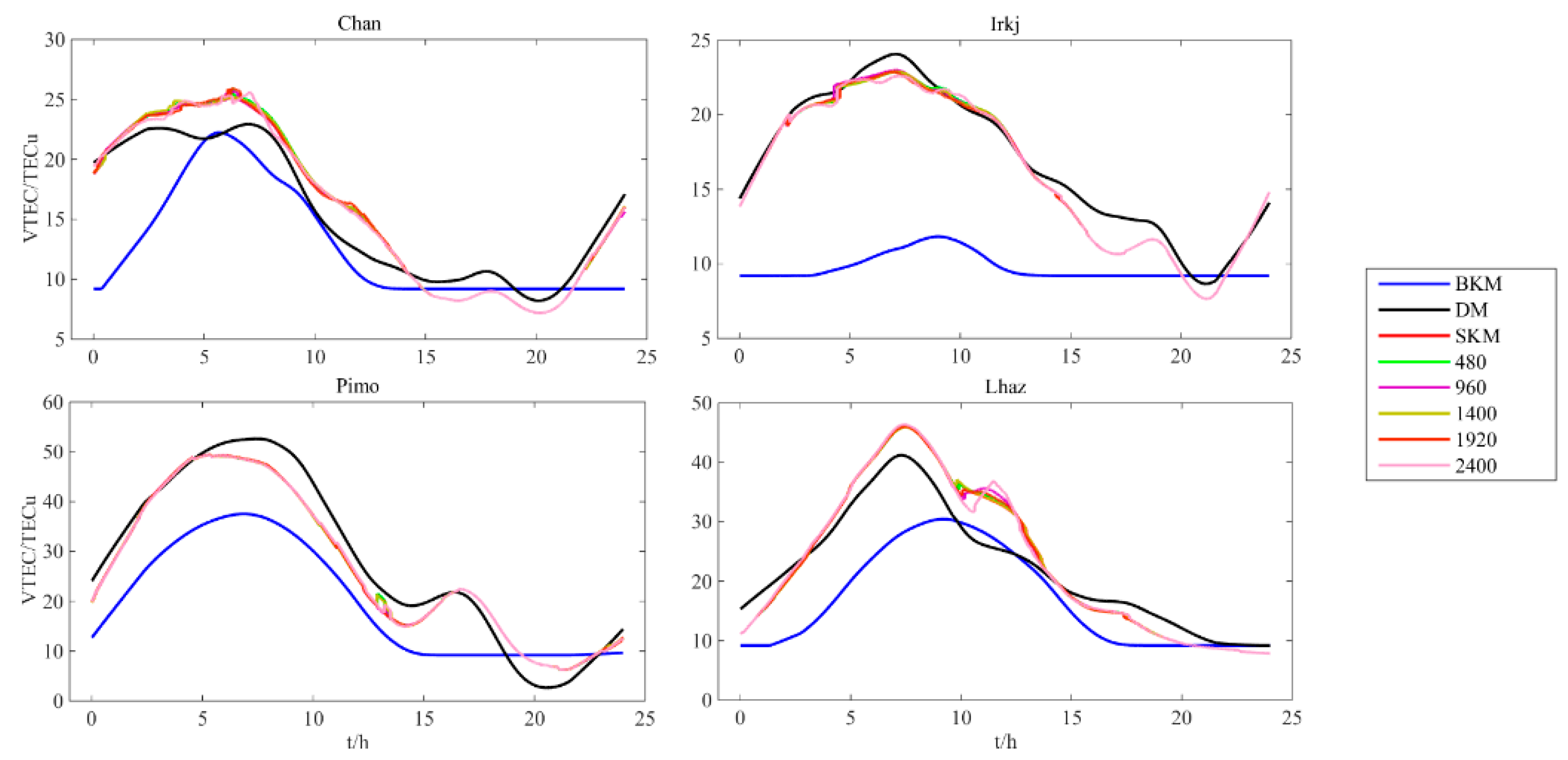
3. Results and Discussion

To establish the sophisticated Klobuchar model over China, this study chooses ten IGS stations within China and seven IGS stations around China (Figure 1). The observation data are from the day of the year (DOY) 095 to 101 in 2011. The sophisticated method of each station is mentioned in Section 2.3. Moreover, this study divides one day into six time periods. Each period contains 4 h (480 epochs). We computed statistical parameters over time periods of 4 h at each station. For each time period, we compute the average bias (Equation (12)) between BKM or SKM and the DM at each station, the average corrective rate (Equation (13)) between BKM or SKM and the DM at each station, and the root mean square error (RMSE, Equation (14)) at each station to test the corrected result. The unit of bias is TECu, the unit of the corrective rate is percentage (%), and the unit of RMSE is TECu. At the same time, a continuous curvature gridding algorithm [43] mapping technique is used to obtain the VTEC over all of China from the isolated point. It is a method that is widely used in earth science and can retain the basic information of each isolated point.

$$bia{s}_{i_j}=\frac{{\sum }_{j=n}^m\left(K_{i_j}-D_j\right)}{m-n},i=1 or 2,$$

(12)

$$P_{i_j}=\frac{{\sum }_{j=n}^m(1-\frac{|K_{i_j}-D_j|}{D_j})\times 100}{m-n},i=1 or 2,$$

(13)

$$RMS{E}_{i_j}=\sqrt{\frac{{\sum }_{j=n}^m\left(K_{i_j}-D_j\right)}{m-n}},i=1 or 2$$

(14)

In Equations (12)–(14), i = 1 denotes BKM; i = 2 denotes SKM; $K_{i_j}$ denotes the VTEC value of BKM or SKM at the j-th epoch; $D_j$ denotes the VTEC value of DM at the j-th epoch; $|K_{i_j}-D_j|$ denotes the absolute error between the two models at the j-th epoch; n denotes the initial epoch; and m denotes the final epoch.

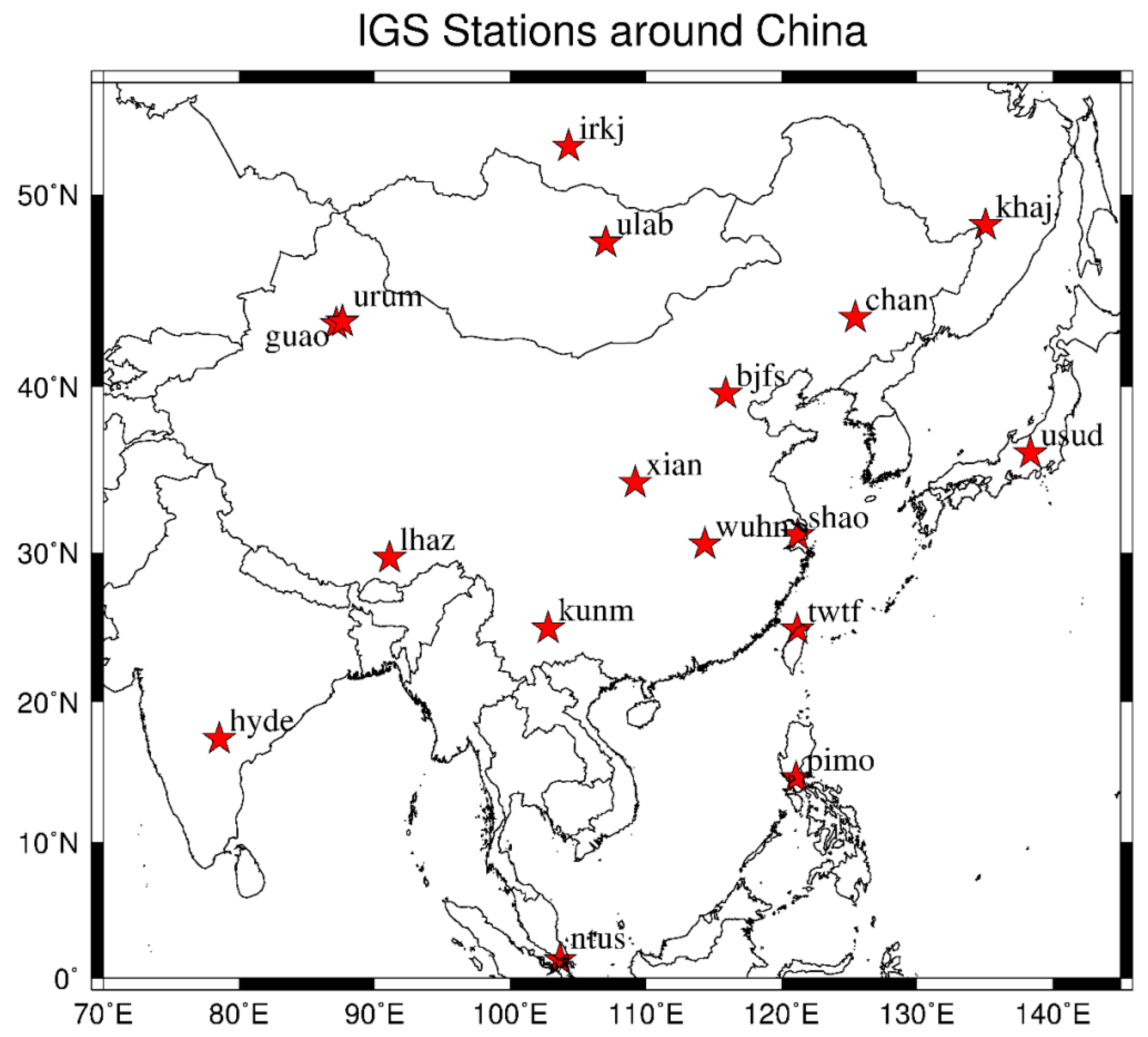
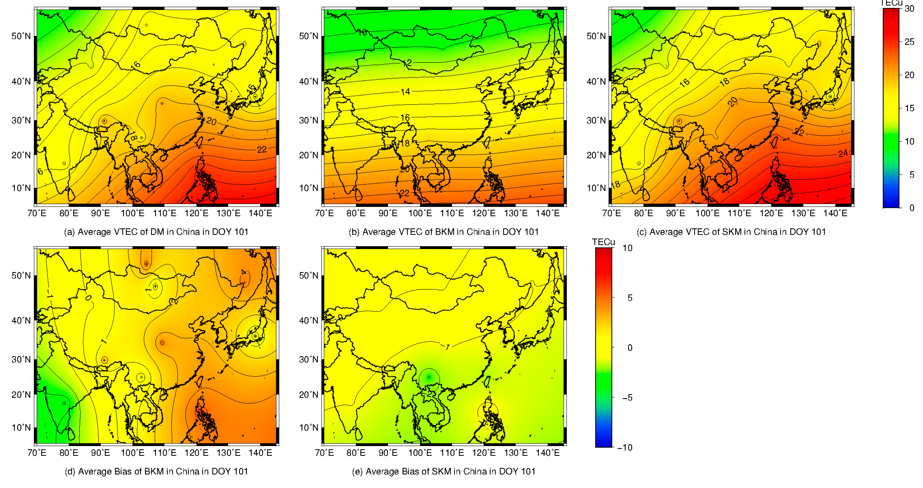
3.1. Result of Modeling in China

The chosen data are used to establish SKM (mentioned in Section 2.3) in the China region. To understand the improvement of SKM, statistical analysis is performed on the average bias between BKM or SKM and DM for DOY 101, 2011; the result is shown in Figure 2. Hence, Figure 2a–c are the distributions of the average values of DM, BKM and SKM in the China region for DOY 101, 2011, respectively. Figure 2d shows that the bias between BKM and DM in China is between −4 TECu and 7 TECu. Among these biases, the largest bias is approximately 6.76 TECu, which appears at the XIAN station. The lowest bias is approximately −3.38 TECu, which appears at the KUNM station. Figure 2d also indicates that BKM has a better correction accuracy in the mid-latitude, but it still needs to be improved; otherwise, the accuracy cannot meet the requirement of high accuracy positioning. Figure 2e shows that the bias of SKM in China is between 0 TECu and 1 TECu. Among these biases, the largest bias is approximately 0.94 TECu, which appears at the GUAO station. The lowest bias is approximately 0.59 TECu, which appears at the KUNM station. Figure 2e indicates that the biases in China improved significantly compared to Figure 2d. Thus, the approach is effective in improving BKM. Moreover, this approach can significantly improve the correction result in the ionosphere.

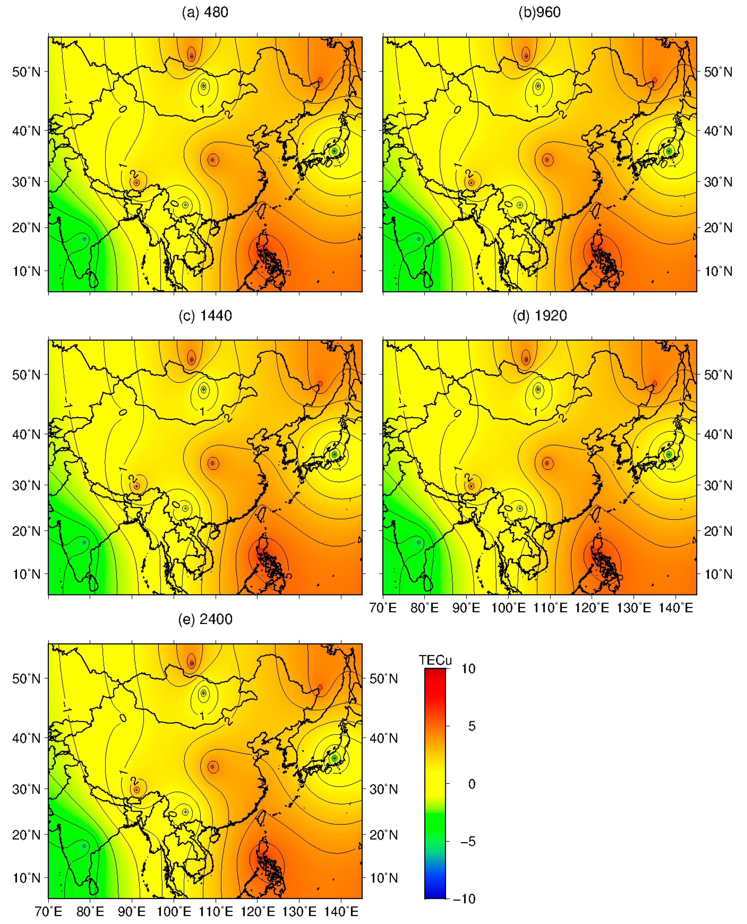
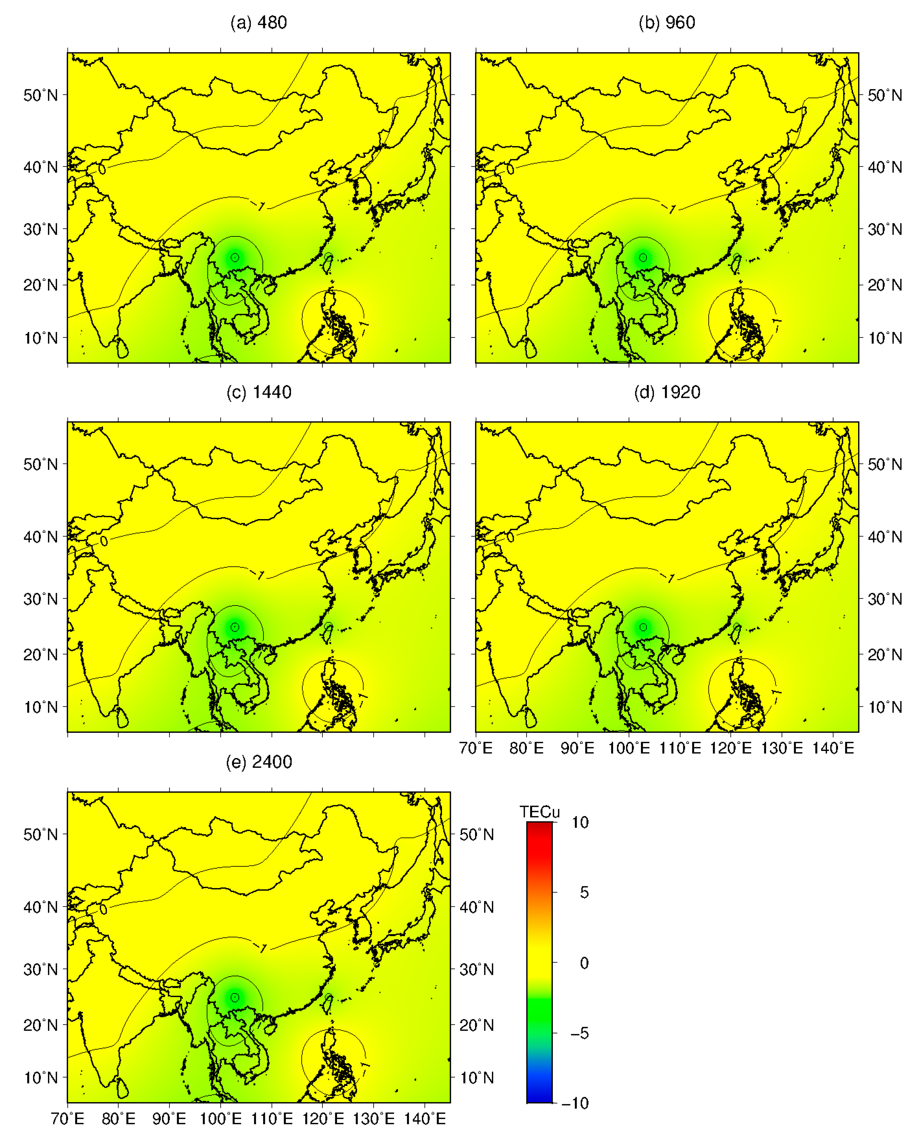
3.2. Result of Modeling in China, Considering Missing Epochs

In Section 3.1, we did not change the sample interval of observation data, with the value remaining at 30 s. Thus, a certain relationship exists between different epochs. However, in practice, some situations may cause the receivers to be unable to accept the signal from the satellite. This weakens the relationship between different epochs and reduces the accuracy of the correcting result, although SKM can achieve a rather good, correct result. This study will consider the applicability of the model for the case of N epochs missing in China.

To determine the accuracy that SKM can achieve while considering epochs missing in the observation data, we consider the following cases: random deletion of 480 epochs (480), 960 epochs (960), 1440 epochs (1440), 1920 epochs (1920), and 2400 epochs (2400). The elimination of random epochs is carried out for each day. For example, random deletion of 480 epochs (480) means that these random 480 epochs are missing for all six previous days. Moreover, cubic spline interpolation is a special case of spline interpolation that is used very often to avoid the problem of Runge’s phenomenon. It gives an interpolating polynomial that is smoother and has a smaller error than some other interpolating polynomials. Therefore, a cubic spline curve [44] is used to restore the missing TEC values calculated by BKM. Next, the TEC values in China are determined using the method described in Section 2.3.

The statistical mean bias is determined for DOY 101, 2011 between BKM or SKM and DM when considering N epochs missing for each of the previous six days in China. The respective results are shown in Figure 3 and Figure 4.

Figure 3 indicates that the distributions of biases between BKM and DM with different epochs missing in China are nearly identical. The biases are between −4 TECu and 7 TECu. Among these biases, the largest bias is approximately 6.80 TECu, which appears at the XIAN station. The lowest bias is approximately −3.40 TECu, which appears at the KUNM station.

Figure 4 suggests that the biases of SKM change little with the increase in the number of missing epochs, regardless of how much of the epoch is missing for each of the previous six days. The biases change in the range of −5 TECu to 1 TECu. In this range, the largest is approximately 0.50 TECu, which was observed at the GUAO station. The lowest is approximately −4.33 TECu, which was observed at the KUNM station. The biases of other stations range from approximately −1 TECu to 0.50 TECu. The correction results of SKM are significantly improvement compared to that of BKM, regardless of how much of each epoch is missing when compared with the results of Figure 3. Moreover, the absolute biases in LHAZ, KUNM and TWTF are larger than those of any other stations. This may be caused by the Equatorial Ionization Anomaly [45].

We can learn from Figure 3 and Figure 4 that the correction result of SKM for China is significantly improved when compared to that of BKM. However, this approach cannot reflect the ionospheric correction result of each time period. Thus, this study counts the correction results from the IRKJ station (LT = UT + 7), the CHAN station (LT = UT + 8), the LHAZ station (LT = UT + 6) and the PIMO (LT = UT + 8) station when N epochs are missing for each of the previous six days. Figure 5 shows the statistical results.

Figure 5 indicates that SKM fits the data of DM well in both the low-latitude and the mid-latitude when no epoch is missing. This shows that SKM can better reflect the temporal variation of the ionosphere, particularly at night. Moreover, the biases between SKM and DM are approximately ±3 TECu in many situations. SKM has a relatively high accuracy with DM. The biases increase as the latitude decreases. In the low-latitude, the biases are larger than that in the mid-latitude. When N epochs are missing in the observation data, the ionospheric correcting accuracy of SKM can also fit the data of DM well in both the low-latitude and the mid-latitude. Moreover, SKM can better reflect the temporal variation, particularly at night. This indicates that the correction accuracy of SKM with N epochs missing is not lower than that of SKM with no epochs missing and can better reflect the temporal variation of the ionosphere, despite the missing epoch. Otherwise, it has little change during the maximum; this behavior may be caused by the exquisite different temporal variations of the ionosphere near the maximum. This influences the forecasting results of the bias and makes the fitted values of SKM approximations near the maximum.

To further show the correction results of SKM with no epochs missing and with N epochs missing, this study counts the average correction results of BKM, SKM with no epoch missing and SKM with N epochs missing for each time period for the IRKJ station, the CHAN station, the LHAZ station and the PIMO station. The statistical results are shown in

Table 1. The statistics of the corrective rate and RMSE for each time period with BKM, SKM and SKM with N epochs missing for each of the previous six days.

Stations	Model	Time Period (Corrective Rate /RMSE)
		0 UT–4 UT	4 UT–8 UT	8 UT–12 UT	12 UT–16 UT	16 UT–20 UT	20 UT–24 UT	Average
IRKJ	BKM	49.5/9.90	45.2/12.65	53.4/9.74	58.6/6.73	73.2/3.55	87.4/2.07	61.2/7.44
	SKM	98.0/0.41	96.7/0.86	98.4/0.40	94.5/1.04	87.0/1.80	93.8/0.67	94.8/0.86
	480	98.0/0.42	96.5/0.90	98.2/0.41	94.5/1.04	87.0/1.80	93.8/0.67	94.7/0.88
	960	98.0/0.42	96.9/0.80	98.5/0.38	94.4/1.05	87.0/1.80	93.8/0.67	94.8/0.85
	1440	98.0/0.41	96.5/0.90	98.4/0.40	94.6/1.04	87.0/1.80	93.8/0.67	94.7/0.87
	1920	98.0/0.42	96.5/0.93	98.5/0.42	94.4/1.05	87.0/1.80	93.8/0.67	94.7/0.88
	2400	97.9/0.44	95.9/1.10	97.8/0.55	94.6/1.04	87.0/1.80	93.8/0.67	94.5/0.93
CHAN	BKM	60.8/8.71	93.5/1.83	91.7/1.62	87.4/1.51	91.1/0.96	78.5/3.79	83.8/3.07
	SKM	95.5/1.12	89.6/2.38	85.2/2.32	87.6/1.65	85.2/1.49	90.0/1.11	88.9/1.68
	480	95.5/1.13	89.0/2.51	85.1/2.33	87.5/1.66	85.2/1.49	90.0/1.70	88.7/1.70
	960	95.3/1.14	89.7/2.40	86.1/2.21	87.7/1.61	85.2/1.49	90.0/1.12	89.0/1.66
	1440	94.8/1.30	89.4/2.43	85.1/2.35	87.6/1.64	85.2/1.49	90.1/1.09	88.7/1.72
	1920	96.0/0.99	89.1/2.54	85.7/2.28	87.1/1.72	85.2/1.49	90.2/1.08	88.9/1.68
	2400	96.5/0.97	89.3/2.46	86.4/2.19	88.1/1.54	85.2/1.49	90.3/1.07	89.3/1.62
LHAZ	BKM	50.8/10.73	64.2/12.88	90.5/4.23	88.8/2.64	63.0/5.81	93.8/1.06	75.2/6.22
	SKM	88.7/2.48	90.5/3.68	77.0/6.81	88.8/3.50	83.0/2.54	86.9/1.38	85.8/3.40
	480	88.7/2.49	90.4/3.70	76.6/6.94	89.3/3.43	83.2/2.56	86.9/1.38	85.8/3.42
	960	88.7/2.48	90.4/3.72	76.2/7.13	89.5/3.50	83.2/2.56	86.9/1.38	85.8/3.46
	1440	88.7/2.49	90.4/3.66	77.0/6.82	88.8/3.51	83.2/2.55	86.9/1.38	85.8/3.40
	1920	88.8/2.47	90.3/3.74	76.9/6.87	89.2/3.48	82.9/2.59	86.9/1.38	85.8/3.42
	2400	89.4/2.39	89.8/3.93	77.7/7.01	90.0/3.44	83.5/2.51	86.9/1.38	86.1/3.44
PIMO	BKM	63.7/12.95	71.0/14.78	69.3/13.39	55.5/9.49	43.1/8.12	-0.49/4.52	49.6/10.54
	SKM	94.5/2.13	95.1/3.06	86.6/5.83	85.2/3.33	64.4/2.93	37.3/2.68	77.2/3.33
	480	94.5/2.12	95.0/3.09	86.5/5.83	85.2/3.32	64.4/2.93	37.4/2.68	77.2/3.33
	960	94.5/2.12	95.1/3.07	86.6/5.81	84.0/3.58	64.4/2.93	37.4/2.68	77.0/3.37
	1440	94.7/2.08	95.1/3.08	86.5/5.85	85.3/3.29	64.4/2.93	37.3/2.68	77.2/3.32
	1920	94.6/2.09	95.2/2.98	86.8/5.73	84.0/3.57	64.4/2.93	36.8/2.71	77.0/3.33
	2400	94.6/2.12	95.1/3.09	87.2/5.65	84.7/3.42	64.4/2.93	36.9/2.69	77.1/3.32

.

Table 1 indicates that the correction results of SKM are significantly improved compared to those of BKM when no epochs are missing. Moreover, the ionospheric correction results in the mid-latitude are better than those in the low-latitude. Moreover, the ionospheric correction results increase with the increase of the latitude. In the low-latitude area (PIMO), the corrective rate of SKM with no epochs missing improved by nearly 30% over BKM, while the RMSE improved by nearly 3 TECu during the day. At night, the corrective rate improved by nearly 30%, while the RMSE improved by nearly 5 TECu. In the mid-latitude area (IRKJ, CHAN, LHAZ), the corrective rate of SKM with no epochs missing improved by nearly 20% compared to BKM, while the RMSE improved by nearly 6 TECu during the day. At night, the corrective rate improved by nearly 30%, while the RMSE improved by nearly 8 TECu. With some epochs missing, the ionospheric correction results of SKM are nearly identical to that of SKM with no epochs missing in both the low-latitude and the mid-latitude, regardless of how many epochs are missing. Among them, the corrective rate changes between −0.5% and 0.5%, with few of the periods changing by more than −1% to 1%. The RMSE changes between −0.1 TECu and 0.1 TECu, with a few of the periods changing by more than −0.2 TECu to 0.2 TECu.

The corrective rate of the low-latitude is better than that of the mid-latitude; however, the low-latitude RMSE is worse than that of the mid-latitude during the maximum values’ time period. This phenomenon is shown in Table 1. This may occur because of the direct influence of the sun. With this influence, the VTEC over stations in the low-latitude areas is larger than that in the mid-latitude areas. This makes the biases between BKM and SKM larger than that in the mid-latitude. Thus, the corrective rate in the low-latitude is higher, whereas the RMSE value is smaller. Otherwise, a negative correction rate value occurs at night, as indicated in Table 1. This may be caused by the constant ionosphere delay value at night. It can also indicate that the constant ionospheric delay value at night cannot accurately reflect the temporal variation at night.

We can also observe from Table 1 that the ionospheric correction results of SKM with N epochs missing are nearly identical to those of SKM with no epochs missing; however, a slight difference remains. This indicates that although the cubic spline curve method has its advantage of being time invariant, the invariance results still exhibit little difference from the observation data. When an epoch is missing, the difference may result in the correction results of SKM with an epoch missing and SKM with no epochs missing to exhibit a bias. The bias may be random.

Recently, many GPS/GNSS users have used dual-frequency receivers or even multi-frequency receivers, and the Continuously Operating Reference Stations (CORS) has been widely applied in many cities. This situation makes it possible and easy to obtain dual-frequency observation data. With these data, it is convenient to calculate the TEC values. Moreover, the corrective bias can be updated once a day. Thus, when users use single-frequency receivers to perform static measurements with a short baseline, observation data are missing because of the sudden change of the surroundings or solar activity. The cubic spline curve method can be used to repair the observation data. With this approach, the missing TEC values can be restored. SKM can be used as a post-correction treatment to address the ionospheric delay value to improve the baseline calculating precision. Moreover, when the single-frequency receivers log in to CORS, the single receivers can obtain the correction value in real time. This approach can reduce the workload of receivers and improve the work efficiency.

4. Conclusions

This study used the observation data from DOY 095 to 101 in 2011 provided by IGS stations within and around the China region to obtain an improved model. In this approach, BKM and DM are used to calculate the TEC values of each day. The TEC value of the previous six days is regarded as input data. The Holt–Winters exponential smoothing model is used to forecast the biases between BKM and DM of the seventh day. The forecast results are used to improve BKM. Moreover, some epochs may be missing in practice because of particular situations, such as sudden change of the surroundings or the activity of the sun. Thus, some epochs are randomly deleted. After we compared SKM with no epochs missing to SKM with an epoch missing with DM via experiments and analyzed the results, we drew the following conclusions:

(1)

SKM with no epoch missing and SKM with an epoch missing can better fit the trend of DM. SKM can better reflect the temporal changes of the ionosphere, especially at night.

(2)

The correction results of the ionospheric delay increase with increasing latitude. All correction results of the ionospheric delay are improved compared to those of BKM during the day. However, at night, the correction results are significantly improved compared to those of BKM. This finding indicates the validity of this method to improve the BKM.

(3)

The cubic spline curve method is used to repair the missing epoch data when the observation data have an epoch missing in some situations. Then, SKM is improved. It can also yield a remarkable result. The correction results of ionospheric delay are nearly identical to those of SKM with no epochs missing, with only a slight difference remaining. This difference may be random.

The analysis presented here shows the results of China over one day. Our conclusions may be limited by the time period and the area. We plan to extend the same analysis to a larger time period and a larger area to validate extensively the SKM algorithm performances. Moreover, we will analyze the impact caused by the update of the eight GPS broadcast coefficients, particularly for the case when there is large variation of these coefficients.

References

1. Zhang, R.; Song, W.W.; Yao, Y.B.; Shi, C.; Lou, Y.D.; Yi, W.T. Modeling regional ionospheric delay with ground-based BeiDou and GPS observations in China. GPS Solut. 2015, 19, 649–658. [Google Scholar] [CrossRef]
2. Ercha, A.; Huang, W.G.; Liu, S.Q.; Shi, L.Q.; Gong, J.C.; Chen, Y.H.; Shen, H. A regional ionospheric TEC mapping technique over China and adjacent areas: GNSS data processing and DINEOF analysis. Sci. China Inform. Sci. 2015, 58, 1–11. [Google Scholar] [CrossRef]
3. Zhao, Q.L.; Wang, G.X.; Liu, Z.Z.; Hu, Z.G.; Dai, Z.Q.; Liu, J.N. Analysis of BeiDou Satellite measurements with code multipath and geometry-free ionosphere-free combinations. Sensors 2016, 16, 123. [Google Scholar] [CrossRef] [PubMed]
4. Hernández-Pajares, M.; Juan, J.M.; Sanz, J.; Aragón-Àngel, A.; García-Rigo, A.; Salazar, D.; Escudero, M. The ionosphere: Effects, GPS modeling and the benefits for space geodetic techniques. J. Geod. 2011, 85, 887–907. [Google Scholar] [CrossRef]
5. Klobuchar, J.A. Ionospheric time delay algorithm for single frequency GNSS Users. IEEE Trans. Aerosp. Elec. Syst. 1987, 23, 325–331. [Google Scholar] [CrossRef]
6. European Commission. European GNSS (Galileo) Open Service–Ionospheric Correction Algorithm for Galileo Single Frequency Users; Issue 1.2; European Commission: Brussels, Belgium, 2016. [Google Scholar]
7. China Satellite Navigation Office (CSNO). BeiDou Navigation Satellite System Signal in Space Interface Control Document-Open Service Signal B1I (Version 2.0); CSNO: Beijing, China, 2012. [Google Scholar]
8. Skone, S.; Yousuf, R.; Coster, A. Performance evaluation of Wide Area Augmentation System for ionospheric storm events. Positioning 2004, 3, 251–258. [Google Scholar] [CrossRef]
9. Migoya-Orué, Y.; Nava, B.; Radicella, S.; Alazo-Cuartas, K. GNSS derived TEC data ingestion into IRI 2012. Adv. Space Res. 2015, 55, 29–41. [Google Scholar] [CrossRef]
10. Daniell, R.E.; Brown, L.D.; Anderson, D.N.; Fox, M.W.; Doherty, P.H.; Decker, D.T.; Sojka, J.J.; Schunk, R.W. Parameterized ionospheric model: A global ionospheric parameterization based on first principles models. Radio Sci. 1995, 30, 1499–1510. [Google Scholar] [CrossRef]
11. Xiang, Y.; Yuan, Y.B.; Li, Z.S.; Wang, N.B. Analysis and validation of different global ionospheric maps (GIMs) over China. Adv. Space Res. 2015, 55, 199–210. [Google Scholar] [CrossRef]
12. Angrisano, A.; Gaglione, S.; Gioia, C.; Massaro, M.; Troisi, S. Benefit of the NeQuick Galileo version in GNSS single-point positioning. Int. J. Navig. Obs. 2013, 2013, 302947. [Google Scholar] [CrossRef]
13. Wang, N.B.; Yuan, Y.B.; Li, Z.S.; Huo, X.L. Impact of ionospheric correction on single-frequency GNSS positioning. In China Satellite Navigation Conference (CSNC) 2013 Proceedings; Springer: Berlin/Heidelberg, Germany, 2013; pp. 471–486. [Google Scholar]
14. Hoque, M.M.; Jakowski, N. An alternative ionospheric correction model for global navigation satellite systems. J. Geod. 2014, 89, 391–406. [Google Scholar] [CrossRef]
15. Wang, N.B.; Yuan, Y.B.; Li, Z.S.; Huo, X.L. Improvement of Klobuchar model for GNSS single-frequency ionospheric delay corrections. Adv. Space Res. 2016, 57, 1555–1569. [Google Scholar] [CrossRef]
16. Li, Z.S.; Yuan, Y.B.; Wang, N.B.; Hernandez-Pajares, M.; Huo, X.L. SHPTS: Towards a new method for generating precise global ionospheric TEC map based on spherical harmonic and generalized trigonometric series functions. J. Geod. 2015, 89, 331–345. [Google Scholar] [CrossRef]
17. Hernández-Pajares, M.; Juan, J.M.; Sanz, J.; Orus, R.; Garcia-Rigo, A.; Feltens, J.; Komjathy, A.; Schaer, S.C.; Krankowski, A. The IGS VTEC maps: A reliable source of ionospheric information since 1998. J. Geod. 2009, 83, 263–275. [Google Scholar] [CrossRef]
18. Gulyaeva, T.L.; Arikan, F.; Hernandez-Pajares, M.; Stanislawska, I. GIM-TEC adaptive ionospheric weather assessment and forecast system. J. Atmos. Sol. Terr. Phys. 2013, 102, 329–340. [Google Scholar] [CrossRef] [Green Version]
19. Macalalad, E.P.; Tsai, L.C.; Wu, J.; Liu, C.H. Application of the TaiWan Ionospheric Model to single-frequency ionospheric delay corrections for GPS positioning. GPS Solut. 2011, 17, 337–346. [Google Scholar] [CrossRef]
20. Komjathy, A. Global Ionospheric Total Electron Content Mapping Using the Global Positioning System; University of New Brunswick: Fredericton, NB, Canada, 1997. [Google Scholar]
21. Liu, Z.Z.; Yang, Z. Anomalies in broadcast ionospheric coefficients recorded by GPS receivers over the past two solar cycles (1992–2013). GPS Solut. 2015, 20, 23–37. [Google Scholar] [CrossRef]
22. Dach, R.; Brockmann, E.; Schaer, S.; Beutler, G.; Meindl, M.; Prange, L. GNSS processing at CODE: Status report. J. Geod. 2009, 83, 353–365. [Google Scholar] [CrossRef]
23. Yuan, Y.B.; Huo, X.; Ou, J.K.; Zhang, K.F.; Chai, Y.J.; Wen, D.B.; Grenfell, R. Refining the Klobuchar ionospheric coefficients based on GPS observations. IEEE Trans. Aerosp. Elec. Syst. 2008, 44, 1498–1510. [Google Scholar] [CrossRef]
24. Wu, X.L.; Hu, X.G.; Wang, G.; Zhong, H.J.; Tang, C.P. Evaluation of COMPASS ionospheric model in GNSS positioning. Adv. Space Res. 2013, 51, 959–968. [Google Scholar] [CrossRef]
25. Rethika, T.; Mishra, S.; Nirmala, S.; Rathnakara, S.C.; Ganeshan, A.S. Single frequency ionospheric error correction using coefficients generated from regional ionospheric data for IRNSS. Indian J. Radio Space Phys. 2013, 43, 125–130. [Google Scholar]
26. Filjar, R.; Kos, T.K.S. Klobuchar-like local model of quiet space weather GPS ionospheric delay for northern Adriatic. J. Navig. 2009, 62, 543–554. [Google Scholar] [CrossRef]
27. Han, L.; Zhang, H.P.; Huang, Y.D.; Wang, M.Y.; Zhu, W.Y.; Ping, J.S. Improving Klobuchar Type Ionospheric Delay Model using 2D GPS TEC over China. In Proceedings of the 36th COSPAR Scientific Assembly, Beijing, China, 16–23 July 2006.
28. Gao, Y.; Liu, Z.Z. Precise ionospheric modelling using regional GPS network data. Positioning 2010, 1, 18–24. [Google Scholar] [CrossRef]
29. Hansen, A.; Blanch, J.; Walter, T. Ionospheric Correction Analysis for WAAS Quiet and Stormy. In Proceedings of the 13th International Technical Meeting of the Satellite Division of the Institute of Navigation (ION GPS 2000), Salt Lake City, UT, USA, 19–22 September 2000.
30. Hatch, R. Synergism of GPS code and carrier measurements. In Proceedings of the 3rd International Geodetic Symposium on Satellite Doppler Positioning, New Mexico State University, Las Cruces, NM, USA, 8–12 Febuary 1982.
31. Hatch, R. Dynamic differential GPS at the centimeter level. In Proceedings of the 4th International Geodetic Symposium on Satellite Positioning, Austin, TX, USA, 28 April–2 May 1986.
32. Lachapelle, G.; Hagglund, J.; Falkenberg, W. GPS land kinematic positioning experiments. In Proceedings of the 4th International Geodetic Symposium on Satellite Positioning, Austin, TX, USA, 28 April–2 May 1986.
33. Liu, Z.Z.; Gao, Y. Ionospheric tomography using GPS measurements. In Proceedings of the International Symposium on Kinematic Systems in Geodesy, Geomatics and Navigation, Banff, AB, Canada, 5–8 June 2001.
34. Sardon, E.; Rius, A.; Zarraoa, N. Estimation of the transmitter and receiver differential biases and the ionospheric total electron from Global Positioning System observations. Radio Sci. 1994, 29, 577–586. [Google Scholar] [CrossRef]
35. Komjathy, A.; Langley, R.B. The effect of shell height on high precision ionospheric modelling using GPS. In Proceedings of the 1996 IGS Workshop, Silver Spring, MD, USA, 19–21 March 1996.
36. Komjathy, A.; Wilson, B.D.; Runge, T.F. A new ionospheric model for wide area differential GPS: The multiple shell approach. In Proceedings of the National Technical Meeting of the Institute of Navigation, San Diego, CA, USA, 28–30 January 2002.
37. Mannucci, A.J.; Wilson, B.D.; Yuan, D.N.; Ho, C.H.; Lindqwister, U.J.; Runge, T.F. A global mapping technique for GPS-derived ionospheric total electron content measurements. Radio Sci. 1998, 33, 565–582. [Google Scholar] [CrossRef]
38. Acob, N.Y.; Abdullah, M.; Ismail, M. Determination of GPS total electron content using single layer model (SLM) ionospheric mapping function. Int. J. Comput. Sci. Netw. Secur. 2008, 8, 154–169. [Google Scholar]
39. Holt, C.C. Forecasting Seasonal and Trends by Exponentially Weighted Moving Averages. Int. J. Forecast. 2004, 20, 5–10. [Google Scholar] [CrossRef]
40. Vroman, P.; Happiette, M.; Rabenasolo, B. Fuzzy Adaptation of the Holt–Winter Model for Textile Sales-forecasting. J. Text. Inst. 1998, 89, 78–89. [Google Scholar] [CrossRef]
41. Kamranrad, R.; Amiri, A. Robust Holt-Winter Based Control Chart for Monitoring Autocorrelated Simple Linear Profiles with Contaminated Data. Sci. Iran. 2016, 23, 1345–1354. [Google Scholar]
42. Kazempour, M.K. Stationary Forecasting; Using Holt-Winter and a Modification of Holt-Winter. Biom. J. 2007, 32, 347–356. [Google Scholar] [CrossRef]
43. Smith, W.H.F.; Wessel, P. Gridding with continuous curvature splines in tension. Geophysics 2012, 55, 293–305. [Google Scholar] [CrossRef]
44. Robinson, M.P.; Fairweather, G. Orthogonal cubic spline collocation solution of underwater acoustic wave propagation problems. J. Comput. Acoust. 2012, 1, 355–370. [Google Scholar] [CrossRef]
45. Paul, K.S.; Das, A.; Ray, S.; Paul, A. Characteristics of Total Electron Content (TEC) observed from a chain of stations near the northern crest of the Equatorial Ionization Anomaly (EIA) along 88.5° E meridian in India. J. Atmos. Sol. Terr. Phys. 2015, 137, 17–28. [Google Scholar] [CrossRef]
Figure 1. The distribution of IGS stations within and around China used to establish the sophisticated model.
Ijgi 06 00075 g001
Figure 2. (a) distribution of average VTEC value of DM in the China region for DOY 101, 2011; (b) distribution of average VTEC value of BKM in the China region for DOY 101, 2011; (c) distribution of average VTEC value of SKM in the China region for DOY 101, 2011; (d) distribution of average bias between BKM and DM in the China region for DOY 101, 2011; and (e) distribution of average bias between SKM and DM in the China region. The color denotes the degree of the bias for DOY 101, 2011.
Ijgi 06 00075 g002
Figure 3. Distribution of mean biases for DOY 101, 2011 between BKM and DM in China when (a) 480 epochs; (b) 960 epochs; (c) 1440 epochs; (d) 1920 epochs; and (e) 2400 epochs are missing for each of the previous six days. The color denotes the degree of bias.
Ijgi 06 00075 g003
Figure 4. Distribution of mean biases for DOY 101, 2011 between SKM and DM over China when (a) 480 epochs; (b) 960 epochs; (c) 1440 epochs; (d) 1920 epochs; and (e) 2400 epochs are missing. The color denotes the degree of bias.
Ijgi 06 00075 g004
Figure 5. Daily variation of vertical TEC at some stations. Top left: CHAN station. Top right: IRKJ station. Bottom left: PIMO station. Bottom right: LHAZ station. Blue lines represent the VTEC values of BKM; black lines represent the VTEC values of SM; red lines represent the VTEC values of SKM with no epochs missing; green lines represent the VTEC values of SKM with 480 epochs missing; purple lines represent the VTEC values of SKM with 960 epochs missing; bottle green lines represent the VTEC values of SKM with 1400 epochs missing; brown lines represent the VTEC values of SKM with 1920 epochs missing; pink lines represent the VTEC values of SKM with 2400 epochs missing.
Ijgi 06 00075 g005