1. Introduction
The automatic generation of 3D models of building exteriors such as facades or roofs in level of detail 3 (LoD3) according to CityGML [
1] has been a subject of intensive research [
2,
3]. For indoor navigation, for example, interior models such as 3D models represented in LoD4 of CityGML [
4] or models acquired from Building Information Modeling (BIM) are required [
5,
6]. In comparison to outdoor models, indoor models are not yet widely available. Indoor models, however, open up new fields of application with high relevance, including indoor navigation, evacuation planning and facility management. In addition, such models are an essential prerequisite for tasks like guide for the blind. While most approaches which derive indoor models rely on measured data such as images or 3D point clouds, we believe that this extensive data acquisition of additional indoor measurements is not necessary. To this aim, we propose a novel method for the derivation of 3D indoor models from sparse observations without the need of extra indoor measurements. If building information models are not available, previous approaches for indoor modeling require indoor measuring and modeling which is both expensive and difficult. Measurements are expensive because each single room has to be accessed. The derivation of models from measurements is difficult due to the masking of walls by furniture. For the distinction between walls and for instance bookshelves or wardrobes, modeling affords prior knowledge and regularization. In this article, we demonstrate that prior knowledge together with outdoor models, especially footprints and information about the positions of windows and floors suffice in many cases if generally available data on room areas, functional use and room numbers are given. To structure and simplify the presentation, we start with the assumption that both floor plans and rooms are rectangular and discuss more general shapes in the end.
The problem we address is characterized by a set of
N rectangular rooms that have to be placed within a polygonal footprint. In this context, a room is defined by a reference point and its width and depth. The width and depth of the rooms are bounded by upper and lower values and constrained by a bilinear constraint
where the area is known a priori and the two parameters
and
are unknown. In the problem we solve, a building footprint as well as the area of each room are given. We assume that each room has a rectangular shape. Lower and upper bounds for the width and depth of each room are derived from probability density functions (PDF). The decision variant of our problem is to decide whether or not the building footprint can be partitioned into rooms that satisfy our specifications. In the special case that the building footprint is a rectangle and that, for each room, the lower bound is equal to the upper bound, this problem is related to Perfect Rectangle Packing. Since Perfect Rectangle Packing is known to be NP-hard [
7], our more general problem seems NP-hard, too. For that reason, it is unlikely to find an efficient solution in the worst case. We understand, however, that an appropriate representation of background knowledge, the definition of domains and constraints on model parameters and an intelligent combination of constraint propagation and stochastic reasoning yields optimal solutions in a rather efficient way in most realistic scenarios. In order to meet these expectations, we propose a method that reduces the search space by a stepwise reasoning. Architectural constraints and regularities together with an initial relaxation of the problem lead to a fast intermediate result that is adapted to a qualified hypothesis in a second step. The relaxation is contributed to the fact that walls are initially not modeled and rooms do not have to fill the entire space. However, an important architectural constraint consists in the fact that interior walls do not intersect windows. In this step, this constraint is reduced to ensuring that interior room boundaries do not cross window ranges. Rooms are modeled in a topological correct way (non-overlapping, within footprint,...) but are not necessarily aligned along a corridor. In the sense of 2D-topological correctness, two rooms are in our context either disjoint or meet each other in common walls avoiding their overlapping. We used a spring model similar to the approach described in [
8]. In this way, we do not consider wall elements in the first step, providing a buffer and enabling improvement of preliminary results in a subsequent step.
Based on the intermediate result, stochastic inference is used in order to deliver a qualified set of solutions that is topologically equivalent but is geometrically different. We use the notion of topological equivalence in the standard sense i.e., equivalent up to homeomorphic transformations (for details, see, for instance, [
9] or [
10]). In particular, topological equivalence preserves adjacency. The set of solutions is augmented by probabilities derived from a most probable estimation. The exact location of rooms—considering an alignment between rooms—, together with its width and depth and the width of walls are estimated in a subsequent step. The key point is the determination of hypotheses together with likelihood information which structures the hypotheses space. In our experiments, we stated that this space is dominated by a hypothesis with regard to others which describes an expected solution.
An extensive analysis of shape and location parameters such as width and depth of rooms leads to a prior knowledge represented by architectural constraints and probability density functions. Similar to the reasoning process performed in [
11], estimation of floor plans is characterized by a bilinear model. The non-linearity is attributed to the fact that a room area is the product of its width and its depth. Besides not allowing that walls cross windows, the fact that windows are e.g., part of office or housing rooms is an important constraint which restricts the domains of shape and location parameters of rooms considerably. Obviously, the latter constraint is not necessary to be hold in the case of corridors or utility rooms. Furthermore, for office buildings with an usually large number of rooms, the available room number is an advantage not to be underestimated since rooms with consequent room numbers tend to be adjacent with high probability. This prior knowledge together with probability density functions make the problem of locating rooms within the footprint feasible. Assigning each window to a room and determining the bilateral relations between rooms turn out to be a combinatorial task that we solved by constraint propagation leading to preliminary topological models.
This paper presents a novel approach for the automatic prediction and generation of building floor plans. Based on sparse observations, we automatically generate a limited number of best hypothesis and provide likelihoods for each solution. The resulted hypotheses are ranked according to an MAP-estimation [
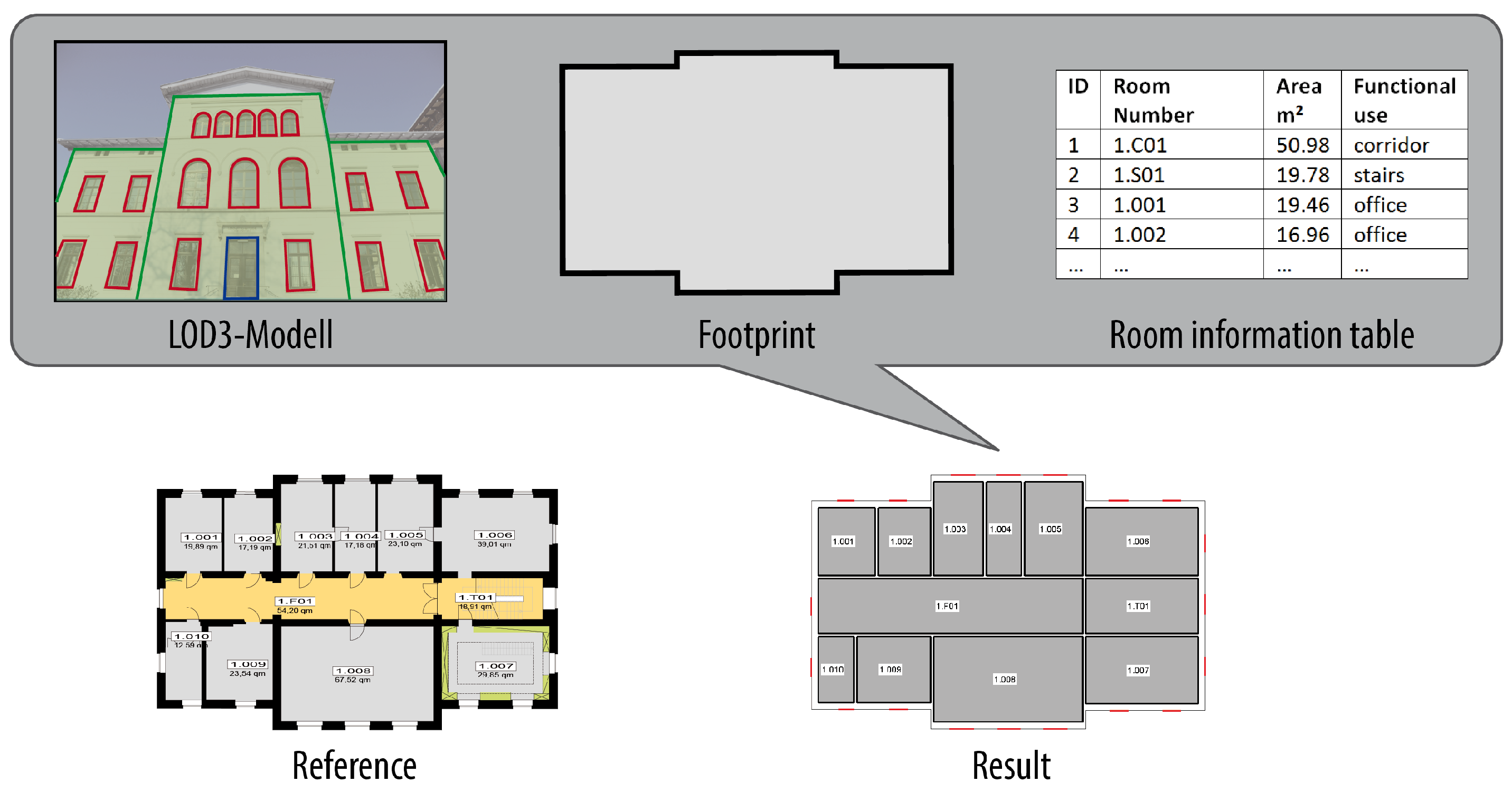
12]. The probability density functions for each model parameter provide the possibility to assess the likelihood of each hypothesis and to order it w.r.t. competitive hypotheses accordingly. Dense observations like 3D point clouds are not required. We understand that it is easier to verify or falsify hypotheses than to reconstruct models from observations in a bottom-up way and follow a model-based top-down approach. While most approaches expect observations of adequate density, characteristic for our approach is that we are able to generate best hypotheses for a floor plan based on otherwise insufficient measurements. We start with geometric information on the building footprint as well as position and sizes of the windows. Furthermore, we exploit non-geometric data on rooms including areas and functional use, at least the distinction between office or housing rooms, corridors and toilet. This is important because, in contrast to office or housing rooms, corridors and toilets do not need windows. As illustrated in
Figure 1, the input consists of a building footprint and available information about rooms (area of rooms, identifying number of each room and possibly the functional use of each room). Most of this information can be acquired from building management services. The location of the windows can be derived using existing methods for the identification of building parts from point clouds or images of facades such as, for instance, described in [
13] or [
14]. The algorithm does not require any indoor images or laser scans from walls to predict, nevertheless, floor plans such as those depicted in
Figure 1. For the comparison, the associated reference floor plan is shown. Additional data may lead to a verification or falsification of models which, however, is less expensive than reconstructing a building interior bottom-up from measurements. The output of our method is an indoor model for the given floor including a layout for the rooms, location of the doors and the height of the rooms. Topology will be consistent and precision of geometry will be optimal w.r.t. the given information due to exact stochastic inference in the sense of [
12]. In our test cases, we yielded accuracies for the model parameters between 10 and 20 cm.
Despite the complex non-linear problem, the presented reasoner performs exact inferences. Therefore, Constraint Logic Programming (CLP) is combined with Graphical models.
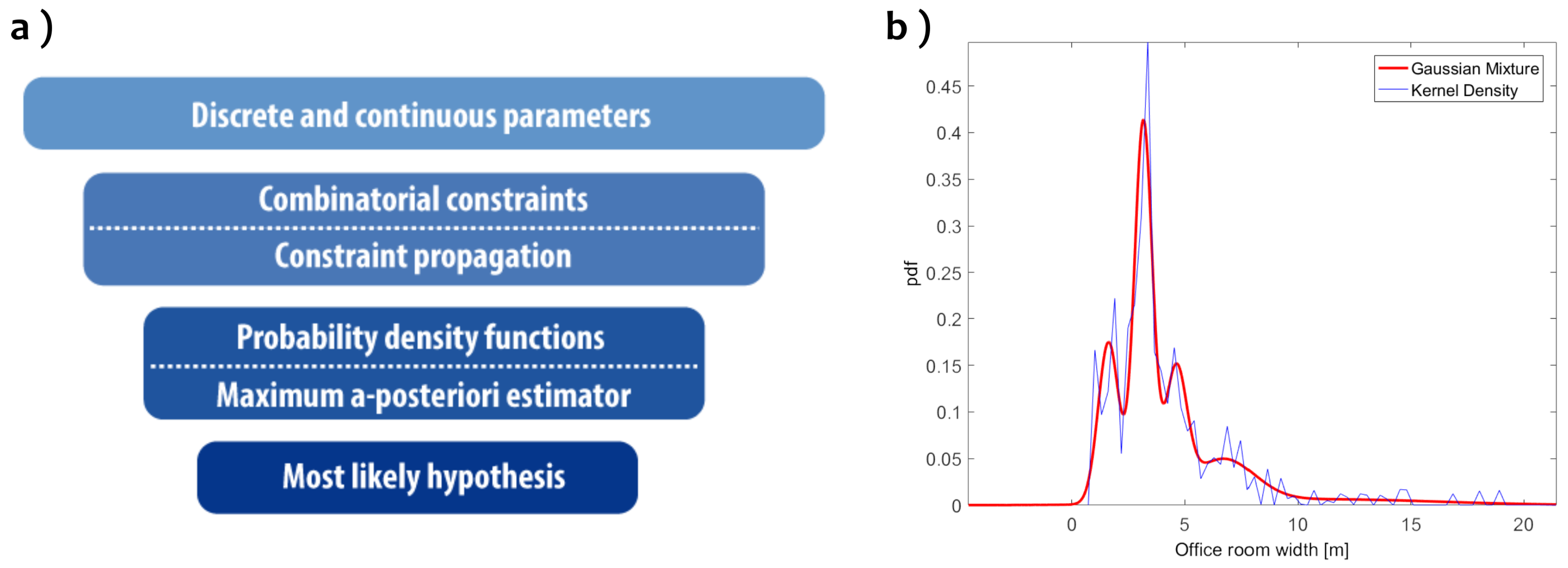
Figure 2a summarizes our general approach: we start with a problem characterized by discrete and continuous parameters and an infinite hypotheses space. This is restricted to a small number of feasible candidates by constraint propagation in a first step. In these hypotheses, model parameters are fixed from a topological point of view, but are intermediate. They are input to a stochastic reasoner in a second step. Parameters are adapted to the available observations and the background knowledge in the form of probability distributions of model parameters by using an MAP-based inference. Probability distributions of model parameters such as the width of office rooms can nicely be represented by kernel density estimations [
15] or—for our purpose even better—Gaussian mixtures, as illustrated by
Figure 2b. It can be seen that the Gaussian mixture is a good approximation to model skew symmetric or multimodal distributions and, at the same time, enables to using well established reasoning algorithms. As stated in [
16], each arbitrary probability density function can be approximated by Gaussian mixture models. We use a special case of graphical models which is a Conditional Linear Gaussian model. This enables performing an exact stochastic inference.
Some of the results described in this paper have been presented at the indoor 3D workshop in the frame of the 11th 3D Geoinfo conference in Athens. This article extends [
17] in several aspects:
The main contribution of this paper is a novel approach which affords 3D indoor models and avoids extra measurements in the form of images or 3D point clouds. From a methodological point of view, we apply stochastic inference in the sense of graphical models and combine combinatorial reasoning/constraint propagation in a bilinear model with stochastic inference using Gaussian mixtures in a novel way. As extension of our previous publication [
17], the approach is described and elaborated in the following sections.
2. Related Work
While 3D models of the exterior of buildings are widely available in different levels of detail, 3D building interior models (LoD4 in CityGML, [
18]) are not yet widespread. Tasks such as rescue management, indoor navigation and guide for the blind have led to growing interest in the design and modeling of building interiors. In this context, the authors of [
19] proposed an approach for the generation of building floor plans from laser range data based on a triangulation of a 2D sampling of wall positions. Becker et al. used shape grammars in [
20] for the reconstruction of 3D indoor models from 3D point clouds. In [
21], Ochmann et al. segmented a point cloud into rooms and outside area and reconstructed the scene by solving a labeling problem based on an energy minimization. For the derivation of indoor models, all mentioned approaches rely on dense observations such as 3D point clouds from laserscans or range cameras using mobile mapping systems. The necessary measurements are both cost and time extensive. Derivation of observations for indoor models is rather different from getting measurements for outdoor models using airborne or terrestrial platforms. Every single room must be entered and scanned. Furthermore, while one is interested in modeling walls, doors, windows and ceilings, they are concealed by all kinds of furniture. Strong model assumptions are needed in any case. In order to overcome the acquisition of dense observations as a time-consuming process, low cost sensors have been employed in several approaches. For instance, Diakité et al. investigated in [
22] the usefulness of the low cost Android tablet from Google’s Tango project for the acquisition of indoor building environments. The information extracted from the native models of this device are not rich enough in order to derive detailed indoor models. As a consequence, our central motivation is to predict unknown substructures in buildings such as floor plans based on strong model assumptions in the sense of background knowledge but only few observations like the area of rooms and footprints. For more information about the works in indoor modeling and mapping, we refer to a survey of recent research in this field [
23].
A constraint-based approach for the generation of floor plans has already been designed in 1994. In [
24], Charmann describes a knowledge-based system that generates all possible floor plans satisfying a set of geometric constraints on the rooms (non-overlap, adjacency, minimal/maximal area, minimal/maximal dimension, etc.). Therefore, he defines the semi-geometric arc-consistency in order to adapt consistency techniques to geometric problems. In comparison to our method, this approach does not address the reconstruction of floor plans for existing buildings and does not take probable configurations into consideration.
Constraint propagation is a powerful method to solve combinatorial problems. Approaches, however, that extend this framework by a stochastic component are rather rare. The authors of [
25] adapt combination and marginalization operators to find the m-best solutions for optimization tasks in graphical models. Intervals with cumulative distribution functions are used in [
26] to model a degree of knowledge for uncertain data. In order to address uncertainty, our approach combines the classical constraint propagation with Bayesian Networks and thus benefits from the strength of both paradigms.
3. Modeling Floor Plans with Constraints
Our approach to predict floor plans follows a model-based top-down approach. Therefore, the problem is modeled based on an extensive analysis of real floor plans as well as dimensional restrictions based on laws and architectural characteristics. We understand that man-made objects are characterized by a number of regularities. On the one hand, geometric relations such as parallelity and orthogonality are dominant in buildings. In [
27], Loch-Dehbi et al. studied the geometric rules that can be found in man-made objects and presented an approach for deducing geometric relations in 3D building models. On the other hand, buildings can be described by functional and statistical dependencies between model parameters. In this paper, we focus on the latter properties of buildings. The knowledge of architectural design as well as available distributions about model parameters enable generation of good hypotheses in order to reconstruct buildings.
The estimation of floor plans can be reduced to find the width
and depth
as well as the reference point
for each single
room. Besides outdoor building models in LOD3, we only need data which is available with every housekeeper and every real estate manager without the need of any indoor measurements. We are given the area of the rooms in addition to the corresponding building footprint and possibly the functional use and the identifying numbers of rooms. Furthermore, we exploit the (two-dimensional) location parameters
and
of the windows stemming from exterior measurements of the facade.
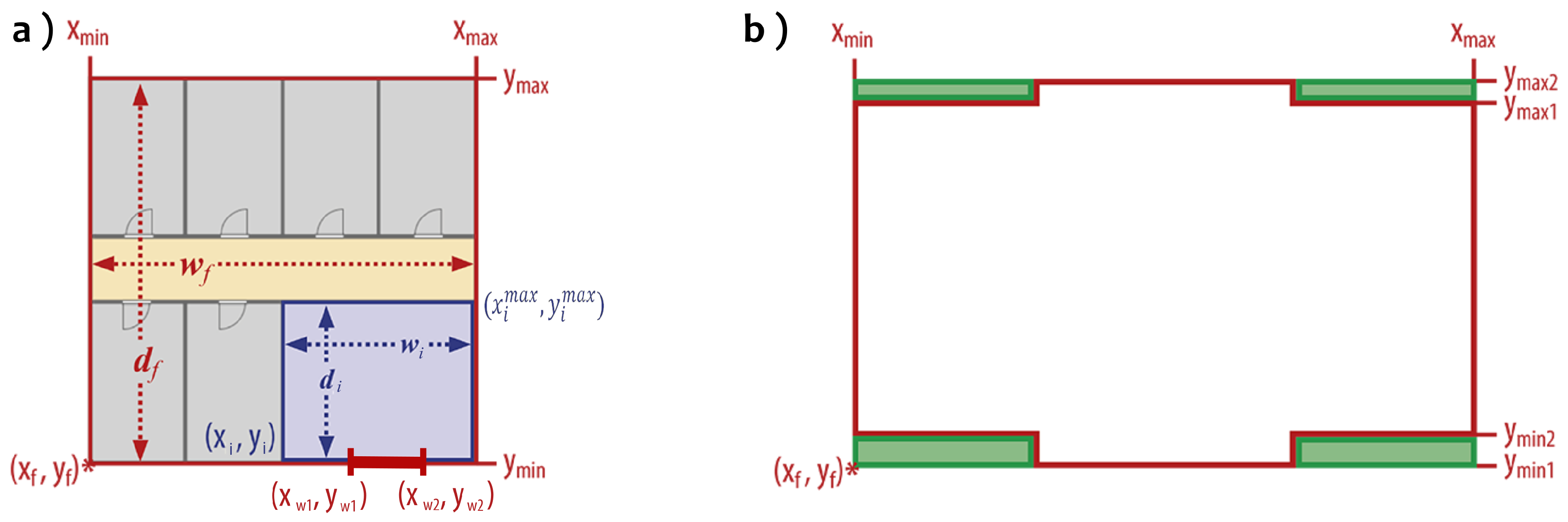
Figure 3a gives an overview of the domain model and its parameters. The figure further illustrates that, for rooms with windows, at least one of their walls has to take the value of the minimum or maximum values
,
,
and
within the corresponding footprint, respectively.
In a first step, we assume that rooms as well as the corresponding footprint have a rectangular shape. This assumption will later be relaxed in order to model buildings that are not rectangular but, however, follow the Manhattan world assumption. Therefore, auxiliary virtual rooms (green rectangles in
Figure 3b can be added that fill the gaps in order to complete a rectangle. Without loss of generality, we further assume that the longest side of a footprint is parallel to the
x-axis in order to have a consistent usage of width and depth for the rooms. For rectangular footprints, this is guaranteed based on an ortho-rectification after a main axis determination of the footprint.
3.1. Hard and Soft Constraints
The topological and architectural knowledge about buildings especially rooms is used to define constraints on the model parameters. In contrast to functions, the constraints usually have several unknown parameters that have to be determined. The first constraint relates the given parameter area of the
room with the two unknowns width
and depth
which is a bilinear, that is non-linear, constraint:
An obvious but important constraint is that all rooms have to be in the (rectangular) floor shape
f derived from the building footprint. It simplifies to a test whether the
room lies within a bounding box with reference point
, width
and depth
. The index
i corresponds to the room identifier in the column ID from the room information table from
Figure 1:
Another important constraint to maintain topological correctness is the non-overlapping of rooms. The fact that two distinct rooms
i and
j have to be disjunct can be modeled as follows:
Knowledge of the positions of windows can be used for two purposes: on the one hand, the coordinates of the rooms depend on the coordinates of the windows which are placed on a shared wall. Consequently, for instance a window
w which lies in the front side of the floor, like the window in
Figure 3, and corresponds to the
room, constrains the possible values of the
y-coordinate of this room in the following way:
where
denotes the depth of the exterior wall. On the other hand, we use the fact that the walls separating rooms do not have to cross windows. Therefore, the
x- and
y-coordinates, respectively, cannot take values where windows are placed. For the same window lying on the front side of the floor, the constraint can be expressed as follows:
For windows of the left, right and back side of a building equivalent constraints exist. Note that the correspondence of a window
w to a room
i expressed by
is as well not known a priori and has to be determined during the reasoning process. This combinatorial task is formulated as a labeling problem. The existence of a window in a room depends on the functional use of this room. For office rooms, an assignment of a window is obligatory, while it is not the case for corridors or utility rooms. If a room is not assigned to a window, it is not constrained by relations (
4) and (
5) and thus can be considered as an interior room.
In addition to the described hard constraints that have to be fulfilled for all rooms obligatory, the floor plan model contains two soft constraints. They hold true in most of the cases but can be violated for exceptions. However, the number of violations is bounded avoiding implausible topological models. One soft constraint considers that the room number is highly correlated to the neighborhood of rooms. If two rooms have consequent room numbers, they should be adjacent where possible. In our context, the term adjacency refers to the neighborhood of rooms. This is expressed by the following constraint—exemplarily for an
room
i left to a
room
j:
where
represents the depth of the interior wall. The symbol “¬” stands for a logical negation. Right, top, and bottom adjacency are also possible and can be defined in an equivalent way. Since the relative relations between rooms are not known, an exclusive-or combines the four possibilities for the adjacency of rooms. This also turns out to be a combinatorial task that we solve.
Since the corridor is usually the entrance to a room, a further soft constraint describes the adjacency of a room to an existing corridor. In this case, the adjacency constraint used for the neighborhood above is conditional on the functional use—in this case “corridor”—of the rooms.
3.2. Probability Density Functions
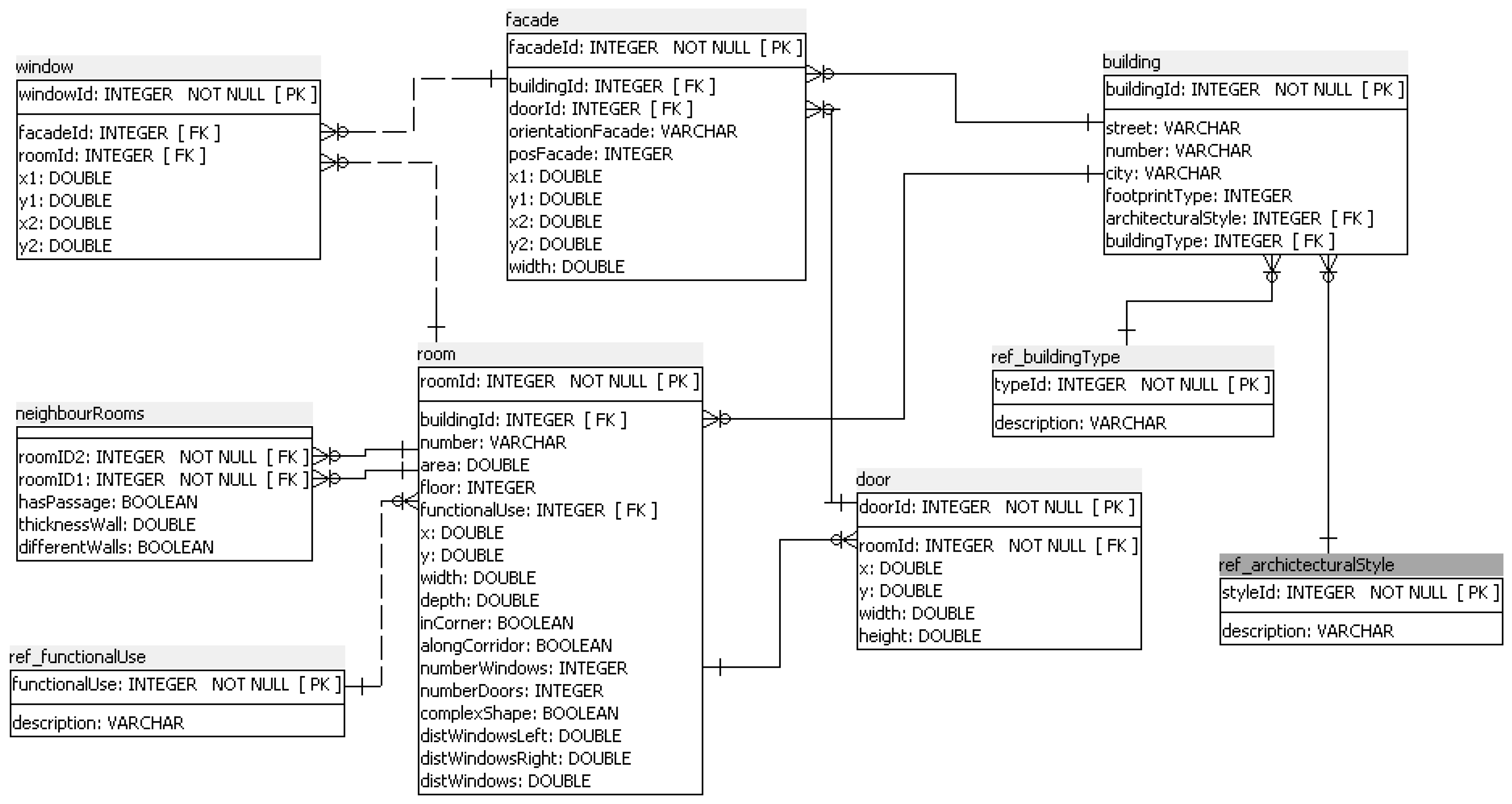
Besides constraints, the reasoning process benefits from statistical prior knowledge that is derived from a groundtruth database of about 1600 rooms with different functional uses.
Figure 4 shows a relevant excerpt of the underlying database model. Central to our analysis is the relation
room with shape and location parameters of each room as well as their functional use and the location of
doors and
windows. Rooms reference their corresponding
buildings, which enables access to available footprints. Finally, the
neighbourhood of rooms is annotated in order to analyze the bilateral locations e.g., with respect to the functional use of rooms. Note that this data does not serve as direct input for the reasoning process but is a representative basis for the derivation of probability distributions and constraints for the floor plan model and its prediction.
As shown in the constraints before, the model is described basically by continuous parameters:
x,
y, width and depth of rooms as well as the depth of exterior and interior walls.
Figure 2b shows the probability density function of the floor plan parameter width of office rooms estimated by the use of kernel densities and compared with its fitted Gaussian mixture. It has been shown that each arbitrary distribution can be approximated by a Gaussian mixture ([
16]):
Gaussian mixtures are an appropriate way to model skew symmetric or multimodal distributions and make it possible to rely on a number of well-studied inference algorithms that are available in literature. By using Expectation Maximization ([
16]), a Gaussian mixture of
m components, each weighted by its probability
for each continuous parameter, is estimated for the reasoning process. On the one hand, probability density functions are used to derive upper and lower bounds for the continuous model parameters during constraint propagation. On the other hand, they are an important knowledge for statistical inference.
4. Constraint Propagation for Topological Floor Plan Derivation
In a first step, the floor plan model is defined by constraints on several variables with associated domains. Constraints described above restrict these domains so that the final solution leads to a small number of qualified hypotheses. In conclusion, our problem can be seen as a constraint satisfaction problem (CSP). Besides the values of the continuous model parameters defining the rooms, we are interested in further discrete parameters. In this context, the correspondence of windows to a room as well as the bilateral relations between rooms have to be determined. This turns out to be a complex combinatorial problem. The idea of our approach is to solve a constraint satisfaction problem with respect to valid values that can be used later on as initial instantiations for statistical reasoning. For solving those combinatorial constraint satisfaction problems, constraint programming is a powerful framework.
A constraint satisfaction problem is characterized by a set of constraints
on domains
of a set of variables
that can be numeric-discrete as well as continuous or symbolic. The Cartesian product of the domains, i.e.,
, defines the initial search space. A
constraint is defined as a relation on a subset of variables
, i.e., a subset of
. They can be boolean or arithmetic—allowing linear as well as non-linear dependencies. A
solution of a CSP is an instantiation of the variables, i.e., an assignment of values for each variable
with
so that all constraints are satisfied. Therefore, the constraint solver follows the “constrain and generate” principle in order to narrow the search space. Constraint inference is performed before finding valid instantiations. During inference, new constraints are derived from existing ones and existing constraints are tightened. This is done by using so called consistency-enforcing algorithms and constraint propagation [
28].
The search benefits from the a priori known domains of the parameters and their constraints. In the context of floor plans, the model parameters of each room are restricted by the bounding box defined by the (rectangular) footprint of the building. The width and depth of the rooms depend on the functional use. For example, toilets usually cannot be as large as lecture halls. Their lower and upper bound can be derived from the Gaussian mixtures estimated by the use of the groundtruth database for rooms. The location of rooms is further bounded by the location of windows that are a priori known from exterior measurements. The constraints described in
Section 3 are used to exclude impossible instantiations by constraint propagation. The latter means deducing additional constraints or restricting existing ones such as narrowing the domains. Herewith, the number of possible solutions is reduced. However, the set of possible solutions can contain those which are not consistent with regard to the constraints. The claim is to omit a subsequent search excluding inconsistencies as early as possible leading to single valued domains. In this context, the search space is affected by the level of consistency. Many domains of constraints can be updated as soon as a related domain changes by considering arc-consistency. A variable
of a (binary) constraint is arc-consistent with respect to another variable
if, for each value of
, there exists an instantiation for
not violating the constraint. However, in some cases, e.g., the equality constraint we use, a more efficient and but sufficiently powerful concept for such consistency-enforcing is to achieve bounds consistency. A constraint
C with
n variables
is
bounds-consistent if for each variable
, there exist instantiations for the other variables
so that
C is satisfiable with respect to the instantiations
and
, respectively.
A and
B denote the lower and upper bound of the associated domain of the variable
represented as an interval. If a bound changes for one variable, new intervals for other variables are calculated by propagation rules in order to reduce the search space within the domains. For instance, for the constraint
(e.g.,
) with
,
and
, the interval bounds for
Z can be updated to
.
A search for solutions is performed by traversing a search graph and finding a solution path to the leaf nodes. A node represents a variable together with one possible instantiation. An arc represents an operator that augments the current solution with a value assignment to an additional variable that does not conflict the prior instantiations regarding the constraints. The search is in general characterized by backtracking. It uses a depth-first search and jumps back to prior states (nodes in the search graph) if the search leads to a dead-end. A dead-end is a leave that is inconsistent with the constraints which means that the domain of its corresponding variable became empty after the constraint propagation. In order to perform a search with as few failures as possible and to avoid backtracking, two principles are followed dynamically during search: Look-ahead and Look-back. The first determines the best choice for the next variable and its value, while the second deals with the level where the algorithm jumps back in case of a dead-end. More details on constraint processing can be found in [
28,
29].
There exist various implementations of constraint solvers [
29]. In addition to algebraic, symbolic or graph-based algorithms, a prominent implementation is Constraint Logic Programming realized by the use of logic programming. CLP benefits from the declarative character of logic programs and the powerful search strategies of constraint programs in order to define and solve constraint satisfaction problems. The search strategy in logic programming is characterized by backtracking with depth-first search. The constraints correspond to relations and predicates in logical language. (Logic) constraint solvers as used in our implementation are powerful tools to handle non-linear constraints with more than one unknown.
The strength of CLP is to solve combinatorial problems in a declarative way. This enables in addition to predefined relations to define customized ones in a simple and flexible way. “Combinatorial problems can be tackled which usually have exponential complexity” [
30]. In our context, we exploit the fact that separating walls of the rooms do not cross windows. We expressed this constraint as a logical relation. Before searching solutions, we enumerate possible (discrete) values for the
x-coordinates of each room excluding those falling within window ranges. Exploiting architectural knowledge, we do not have to cope with the a priori infinite continuous search space. Instead, we transfer the problem into an enumeration of interesting values so that the search algorithm finds the arrangement of the rooms much faster than dealing with infinite continuous domains. The most important value is the one that lies in the middle between two windows. This is attributed to the fact that most of the walls are centered between windows. This high level of discretization is especially valid for rooms that obligatory have a window such as office rooms. Other rooms of different functional use e.g., corridors are excluded and their domains are represented by intervals with decimeter precision. This is necessary since the reference points of corridors can take values that are excluded by the windows for other rooms.
The discretization along the
x-axis leads to an easier instantiation of the other parameters. If, for the
room,
and
are determined, the width
can be subsequently derived (cf.
Figure 3). Likewise, the assignment of the depth follows from a previous assignment of the width according to the constraint
. Following this pattern, we are transforming constraints into functions with only one unknown parameter. The
y-coordinate
is determined by the corresponding window, that is the minimum
or the maximum
of the footprint respectively, depending on the window location. If the window lies on the front side of the floor,
equals the lower bound
of the floor. Otherwise, if the window is located on the opposite side,
equals
.
We are aware that the transition from continuous to discrete values does not guarantee to match the expected values. We ignored temporary the walls in order to provide buffers for the deviations occurred after the value discretization. In this context, the variables
and
have not to be determined in this step. As a consequence, irregular gaps exist between the rooms and the alignment of rooms along the corridor is not automatically given. Furthermore, uncertain measurements were not considered during the combinatorial reasoning.
Figure 5 shows in the second row the intermediate result that is found by constraint propagation. Although the result is topologically correct and satisfies the given constraints defining the floor plan model, it has to be adapted geometrically in a subsequent step. This will be elaborated in the next section.
5. Conditional Linear Gaussian Models for Stochastic Floor Plan Prediction
As stated in the previous section, constraint propagation yields an intermediate result with a correct topology, but suboptimal geometrical parameters. The predicted preliminary rooms do not fill the entire footprint space. In particular, the alignment of rooms along a corridor is not guaranteed. The combinatorial reasoning provides initial values that are updated and refined. The result remains topologically equivalent but becomes geometrically different in order to match the provided measurements. After tackling the combinatorial task leading to a consistent solution from a topological point of view, we focus on closing the gaps between the rooms. In this stage, exact inference can be performed in order to satisfy this task.
The inference is realized in the frame of a stochastic reasoning which gives access to well known statistical algorithms. The functional model is defined basically by two types of constraints that ensure the geometrical consistency. The most important constraint describes the local relation between two adjacent rooms. We exploit the fact that the combinatorial component finds the bilateral relations between rooms. For example, if the
room is left to the
room, then their coordinates are related by:
This constraint enforces not only the adjacency between rooms but also the alignment of rooms along corridors. This is a consequence of the rectangular shaped rooms according to the Manhattan world assumption. It should be noted that constraint (
8) is a part of constraint (
6) since topological aspects do not have to be considered anymore.
Similar to the constraint (
4), the exact location of the reference point of each room is corrected exploiting the information about windows’ correspondences to rooms from the combinatorial part:
Again, this constraint exemplarily holds for windows (and their associated rooms) that lie on the front side of the floor.
In order to perform a stochastic reasoning, we make use of probability density functions addressing the uncertainty of the model parameters. It can be stated that the prior knowledge is in principle neither Gaussian nor unimodal. This statement can be confirmed in
Figure 2b exemplified by the room width as an important part of our stochastic background knowledge. Non-Gaussian and multimodal distributions are known to not be suitable for efficient and exact reasoning. We mentioned already that we overcome this obstacle by using Gaussian mixtures. When we use the intermediate model of the combinatorial part as a starting point for the stochastic estimation of geometric parameters, each model parameter is related to one component of a Gaussian mixture. Using this approach, we can safely assume that parameters are normally distributed in the following and are no longer multimodal. We are now in a special, well-understood field of stochastic reasoning with probabilistic graphical models.
Probabilistic graphical models are nowadays one of the most prominent and most powerful methods for reasoning in uncertain domains. Bayesian Networks are one type of graphical model represented by directed graphs, where each node
is related to a random variable
and where the absence of edges indicates independencies between these model parameters ([
12]). Random variables are characterized by conditional probability distributions (CPD)
that give probabilities for each variable status dependent on the instantiation of its parent nodes
, which are its immediate predecessors as induced by the graph. The graph structure enables a compact representation of a joint distribution and paves the way for an efficient inference in order to determine the posterior distribution given an observation. The presented floor plan model is defined by constraints on discrete as well as continuous variables and thus has to be represented by hybrid networks that are characterized by nodes associated with discrete as well as continuous variables
. In contrast to approximate reasoning, exact inference within hybrid networks is in general not feasible. The feasibility is achieved with additional assumptions such as that a parameter
X is normally distributed with mean
μ and variance
:
A special case of Bayesian Networks is the conditional linear Gaussian (CLG) network ([
31,
32]) that assumes Gaussian distributions for the continuous parameters. All continuous variables have to be described by conditional linear Gaussian CPDs, and their corresponding continuous nodes are not allowed to be a parent of a discrete node. A conditional linear Gaussian CPD with
and
is defined as
where
is a mean value for instantiation
τ,
a vector of regression coefficients and
the corresponding variance.
The joint distribution in a hybrid network can thus be defined as an
-dimensional Gaussian distribution
for each instantiation
τ of
([
33]).
In the context of floor plan modeling, our problem fits well the assumptions on CLGs. Therefore, we use a CLG network in order to model uncertainty and improve the intermediate result from the CLP. The selection of the components of the Gaussian mixtures allows us to use a specially structured Bayesian Network: a state-observation model with an n-dimensional state vector representing the model parameters and an m-dimensional observation vector that can be described by the mapping with a measurement matrix . For such state estimations, the correction step of Kalman filter is an efficient algorithm for calculating the posterior. It assumes that state transition and measurement can be described linearly and initial beliefs are represented by multivariate Gaussian distributions.
In our context, Gaussian distributions with
μ and
σ are carried over from the constraint solver of the reasoner and are augmented by two dimensions in order to model the exterior and interior walls. The functional model represented by the measurement matrix
M is defined according to Equations (
8) and (
9). It should be noted that in this case compared to Equation (
6), the equality of parameters is converted into a substraction that equals zero. In this way, the state-observation model can be used with a pseudo-observation equal to zero. The posterior is computed by matrix multiplications similar to the correction step of the Kalman filter. The Kalman gain
is used to update, that is, to adjust the intermediate result of the combinatorial component and the Gaussian distributions are updated by
where
is the Gaussian noise of the observations and Id is the identity matrix.
Finally, the most likely assignment (MAP assignment) for given evidence is found by maximizing the posterior probability for variables : . The presented work aims to find the k most probable explanations, denoted by in order to assess the quality of the solutions.
The reasoner provides means
for continuous model parameters of the
hypothesis and the related instantiations
for discrete variables. Final hypotheses are ordered by their (unnormalized) probabilities
calculated on the basis of the a priori known distributions:
where
is the on
scaled density of the distribution corresponding to the
model parameter. We finally get a set of hypotheses of the most probable floor plans given the observations:
Since, in this stage, we can assume Gaussian distributions, likelihood of hypotheses is calculated based on the given covariance matrices and the residuals in the ordinary way. The probability density functions for each model parameter provide the possibility to assess the likelihood of each hypothesis and order them accordingly.
6. Results and Discussion
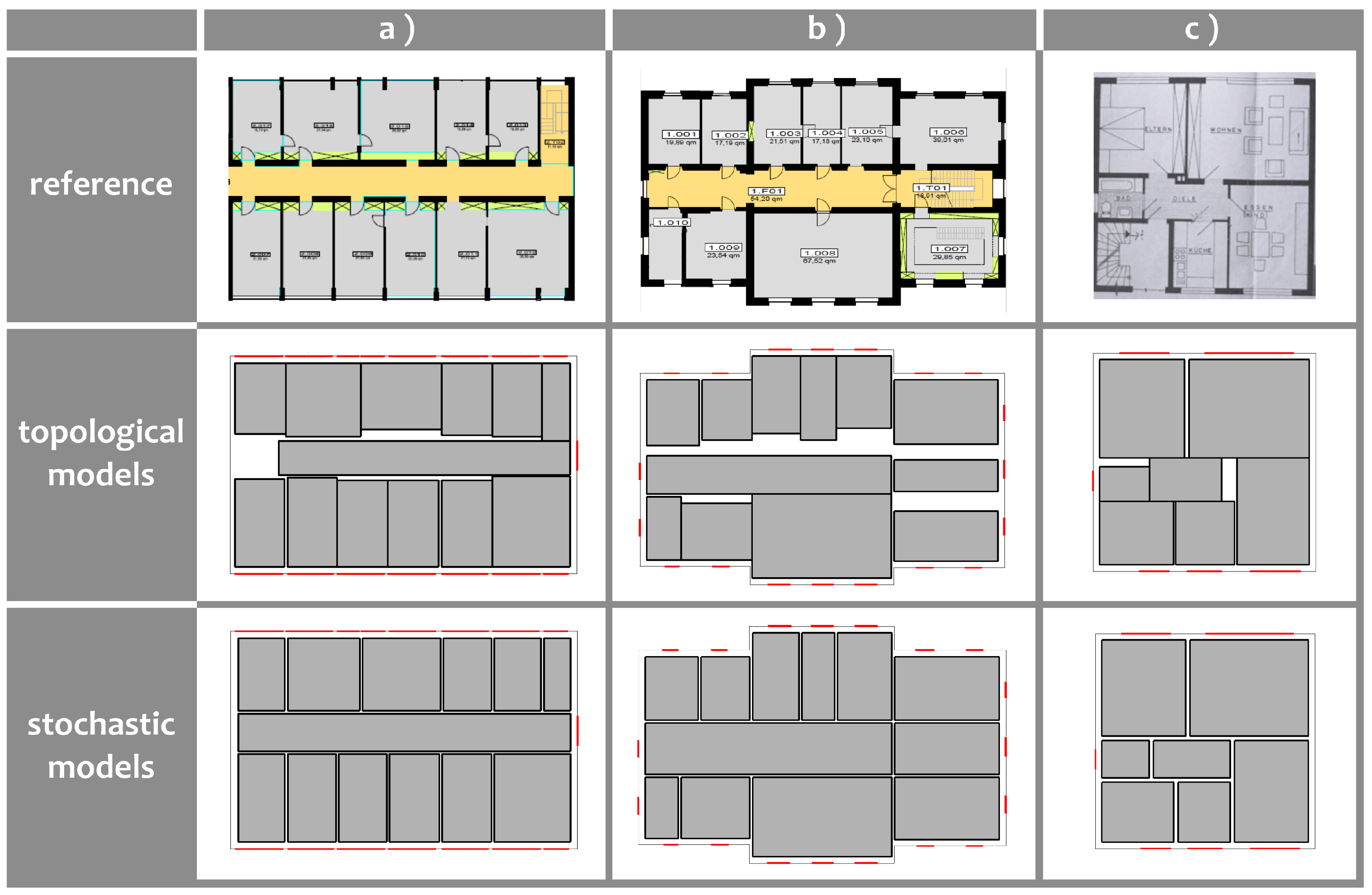
As a result, the reasoner yields automatically the most probable floor plans in significantly less than a second in nearly all cases on a Windows 64 Bit machine (3.4 GHz, 16 GB RAM). We assumed standard deviations of 10 cm for the location of windows and yielded, in our test cases, accuracies for the model parameters between 10 and 20 cm. The results are summarized in
Figure 5. Each predicted floor plan in the last row corresponds to the best ranked hypothesis found by our approach. The second row shows the intermediate results provided by the constraint propagation. For comparison, the reference floor plans are depicted in the first row. The quality of the results depends on how much the floor plans meet the norm with respect to the distributions derived from the prior knowledge.
It can be seen that the reasoning component in the combinatorial part estimates the correspondence of windows to rooms and determines the approximate location of each room. Not modeling the interior walls provides a buffer which supports preserving topological correctness. Geometric consistency is considered in the next step as well. The statistical component fills the gaps by adjusting the shape and location parameters and the depth of walls. The alignments of rooms along existing corridors are ensured as well. The listed results of our reasoning process show exemplarily floor plans predicted with regard to different requirements. The first column depicts a rectangular floor plan stemming from an office building. Most of the buildings are characterized by a rectangular shape. The second column shows a floor plan that does not satisfy the rectangularity assumption. In this case, it is adapted to a rectangular shape by adding four auxiliary rooms. Nevertheless, the non-rectangularity turns out to be beneficial and can be exploited to determine grid points for the discretization of the x-coordinate. While a simple unstructured rectangular footprint provides no information about walls, in this case, the left and right boundaries of the protrusions indicate an interior wall as a bound for a room at this position. The last row visualizes the results of the reasoning for a floor plan in a residential house. The particularity for this type of floor plan is that the rooms usually do not have an identifying number that could restrict their location.
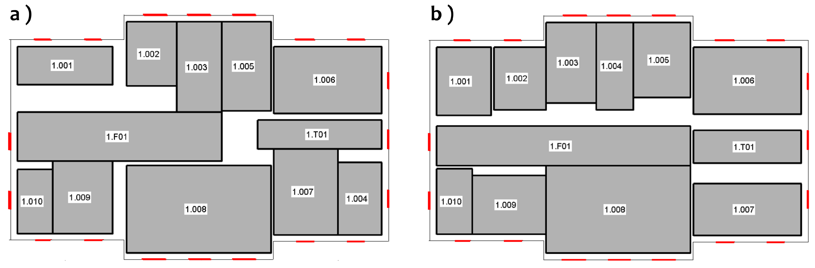
How the knowledge about room numbers influences the prediction is shown in
Figure 6. Due to the soft constraint of adjacent rooms in the case of consequent room numbers, the reasoner finds the correct ordering of the rooms and thus predicts the floor plan. The left result is avoided using an upper bound for the number of the violations of the soft constraint so that only rooms 1.006 and 1.007 are not adjacent. Furthermore, the knowledge of one single correspondence of a room to a window accelerates the reasoning process. This fact is especially beneficial for rooms whose associated windows are easily identifiable from outside, such as the case of stairs.
Derivation of a 3D Indoor Model from Predicted Floor Plans
Up to now, we have described how floor plans can be estimated without any indoor measurements. This 2D model is extended to a 3D model by extruding the walls of the rooms and inserting windows and doors. Windows are known a priori from outdoor measurements. Doors can be predicted due to available distributions of the location of doors from annotated data.
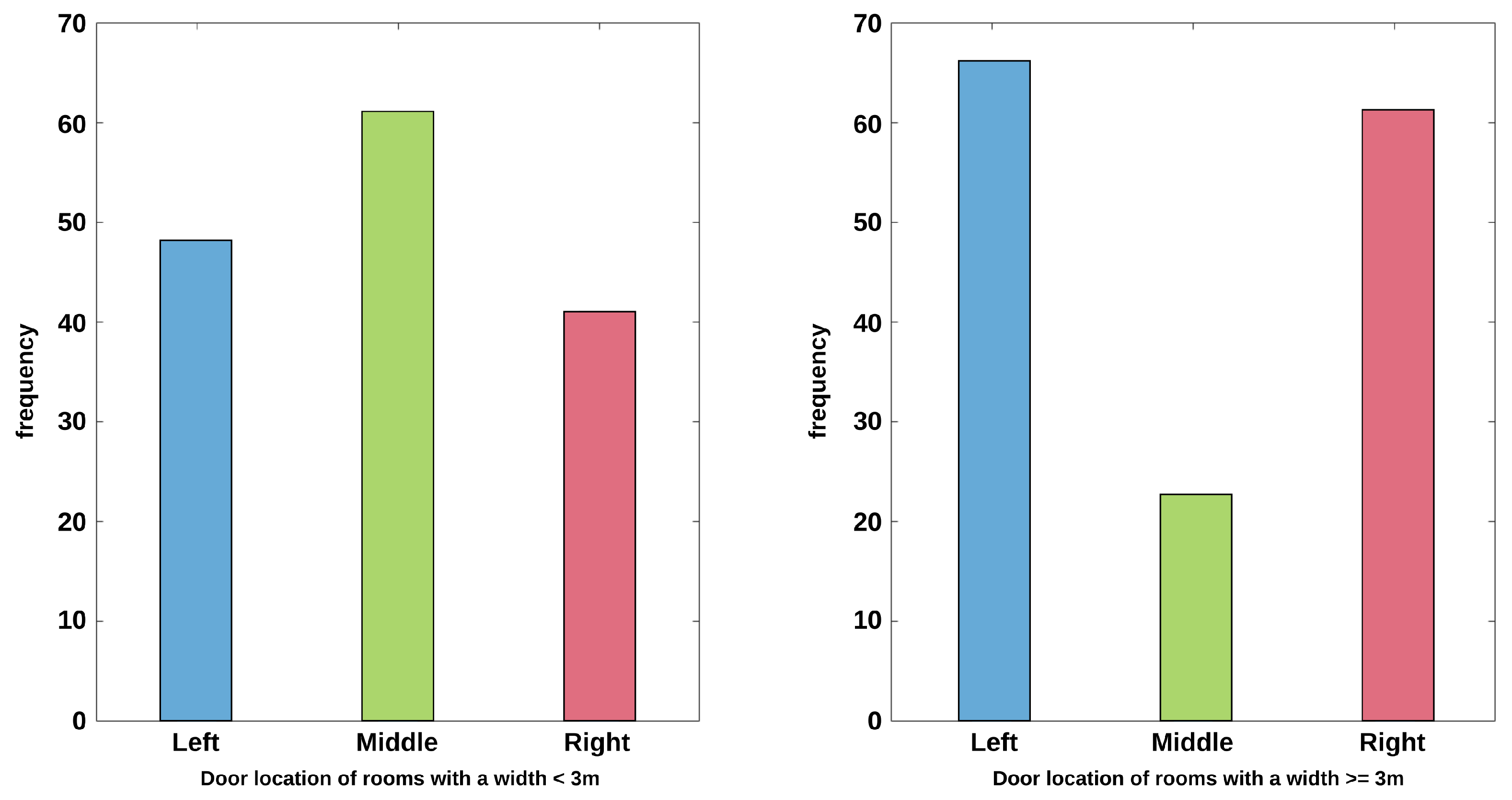
Figure 7 shows these distributions, where possible locations of a door are divided into left, right or middle. Hypotheses are derived depending on the size of the rooms, which influences the distribution.
The height of the walls in turn is derived from the height of the facade and the location of windows. As described in [
13], the height of each story can easily be derived by kernel density estimations based on 3D point clouds of facades. Since windows are usually located at hip height, the knowledge can be exploited to predict the location of the floor within the building.
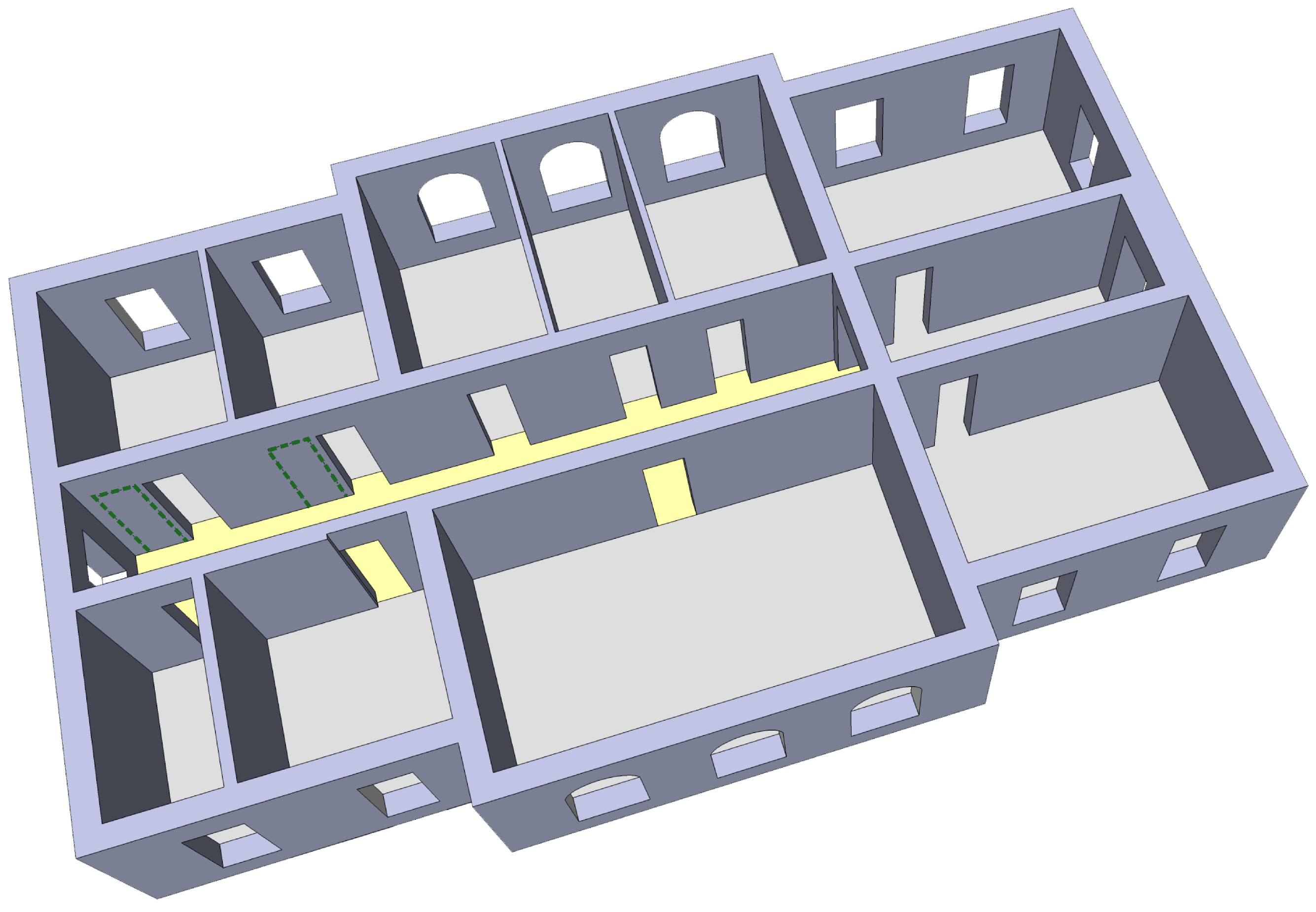
Figure 8 shows the 3D indoor model corresponding to the floor plan derived in
Figure 5b. In rooms with a width smaller than 3 m, doors are mostly located in the middle of the wall shared with the corridor. In larger rooms, the histogram shows that the left and right position of the door is more probable. The doors in our 3D model are predicted based on these distributions. Special rules are introduced in order to model architectural features. For example, for the rooms at the right side of the building, doors cannot be located close to the right wall, as indicated by the learned distribution, since the stairs would avoid this placing (cf. reference image in
Figure 5b. Furthermore, in small toilets, such as room 1.010, the door does not lie in the middle since the space should be used to place a sink close to the door. A courtroom in cultural heritage buildings, such as the case here, usually has the door centered in the wall while lecture halls or auditoriums locate the door at the left or right side due to the rows of chairs and their accessing corridor. False positives of our door prediction are marked with green dotted lines. Future work will take this issue into account based on a supervised classification task in order to predict doors in a more robust way.
7. Conclusions
The paper presents a novel approach for the prediction of floor plans without the need of any indoor measurements. The algorithm represents prior knowledge with probability distributions of the model parameters on the one hand and linear as well as bilinear constraints on the other hand, using an extensive data analysis. This analysis is based on a large database of about 1600 buildings, which captures, among others, shape and location parameters of the rooms. Parameter distributions are represented by Gaussian mixtures that are flexible enough to model multi-modal distributions on the one hand, and can be reduced in our approach to single Gaussian distributions allowing exact stochastic inference on the other hand. Constraints together with probability density functions reduce the search space and enable reconstruction of floor plans based on otherwise insufficient data.
In order to be able to apply exact stochastic inference in complex models, we combine constraint processing with a conditional linear Gaussian graphical model. The combinatorial problem of assigning each window to a room and determining the bilateral relations between rooms is solved by constraint propagation, leading to preliminary topological models. This intermediate result is adjusted by a statistical component that aligns rooms along corridors where possible and estimates walls completing the floor plan model.
Initially, we had assumed that floor plans and rooms are rectangular.
Figure 8, however, illustrates how an extension allows more general shapes of floor plans. We are aware that there are more general room layouts such as L, T or even U shaped rooms. Despite these shapes of rooms seeming to violate basic assumptions on general approaches, we believe that they can be modeled as a composition of two or more rectangular rooms. Whereas the stochastic modeling seems to be feasible, the modeling and design of constraints for a constraint solver will be a subject of future work.
Based on the predicted floor plans, a 3D indoor model is built with the use of architectural regularities and probability distributions exploited for the prediction of doors. The floor heights are extracted from the distances between windows from subsequent floors. The door locations are predicted using Gaussian mixtures, whereas the shape parameters of doors are derived from probability density functions depending on the building style.
In this paper, the examples have been chosen in such a way that they represent rectangular models that cover a significant part of office rooms as well as non-rectangular floor plans. We took not only post-war building styles into consideration, but also buildings stemming from the beginning of the last century. The paper dealt also with residential houses. More complex room layouts in this context will be the topic of a forthcoming paper.
Recently, the integration of BIM and outdoor models in the CityGML format have gained more attention. BIM is a hot topic in the context of construction industry and supports both the construction process and facility management. While, in the recent past, models in the geoinformation and CityGML context focused on the outer building surfaces, constructive aspects and building indoors are the main points of interest from a BIM point of view. We believe that, in cases where BIM models are not available, our approach that predicts indoor models without additional measurements provides a link between BIM and CityGML.

