
Integrating Geospatial Techniques for Urban Land Use Classification in the Developing Sub-Saharan African City of Lusaka, Zambia


Abstract
:1. Introduction
2. Study Area and Data
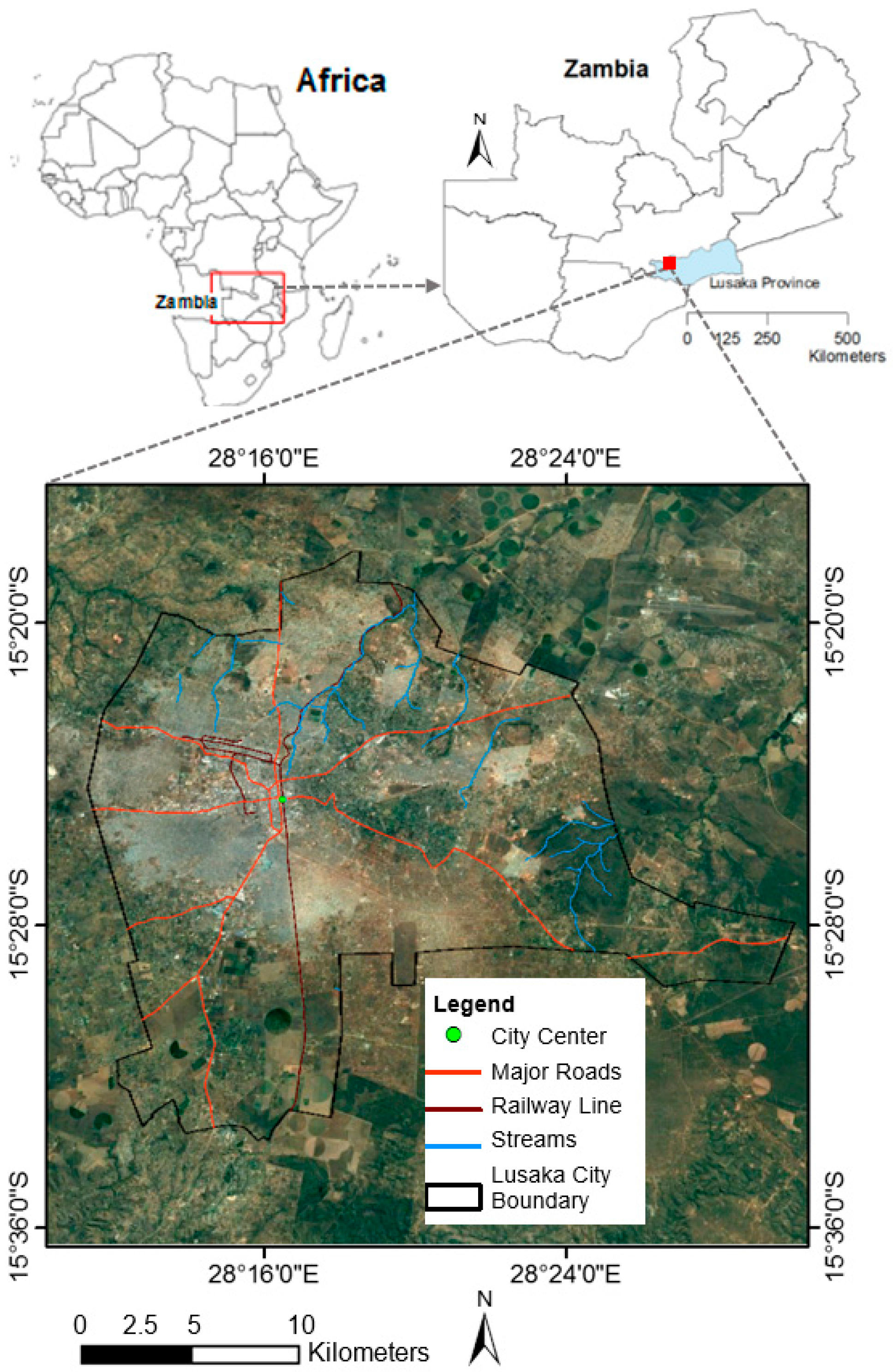
2.1. Study Area
2.2. Data
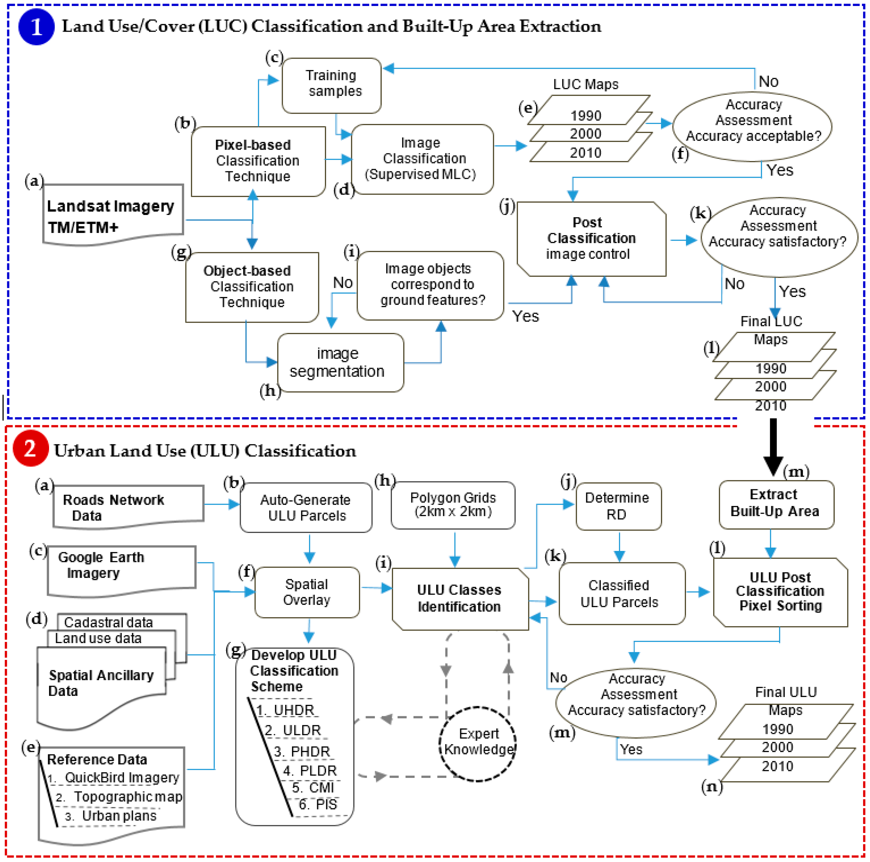
3. Methods
3.1. LUC Classification and Built Area Extraction
3.1.1. Pixel-Based Classification
3.1.2. Object-Based Classification
3.1.3. Post-Classification
3.1.4. LUC Classification Accuracy Assessment
3.2. ULU Classification
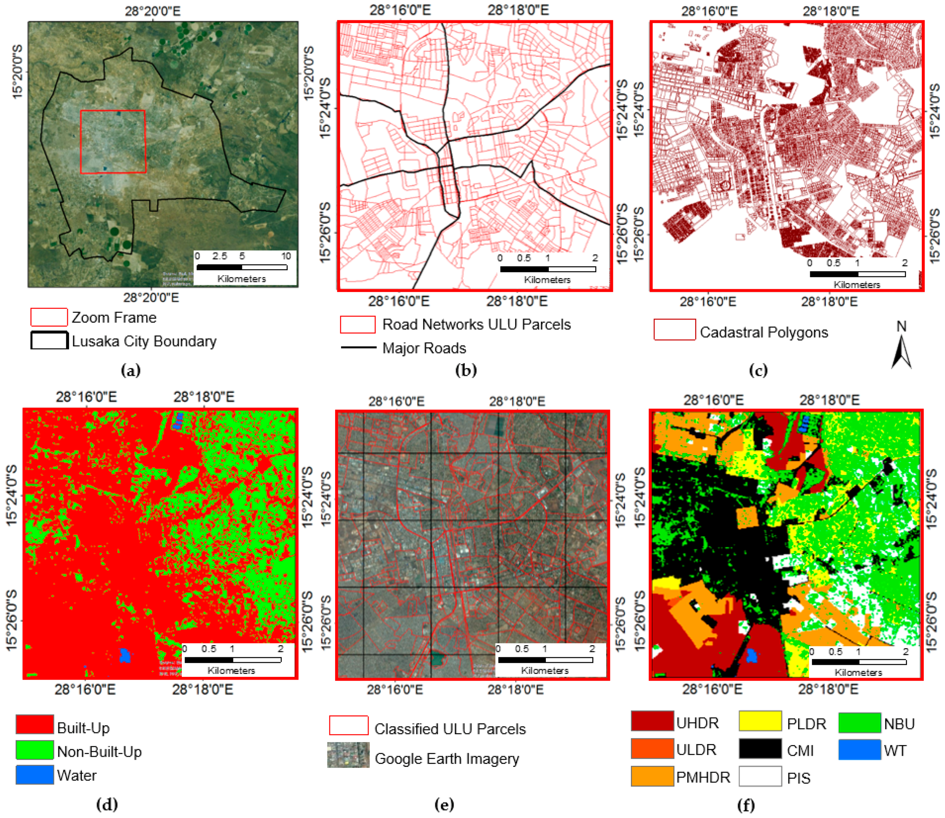
3.2.1. Classification Scheme
3.2.2. Creating ULU Parcels
3.2.3. Identification of ULU Classes
3.2.4. Determining Residential Density
3.2.5. Post-Classification Pixel Sorting
3.2.6. Accuracy Assessment and Hypothesis Validation
4. Results
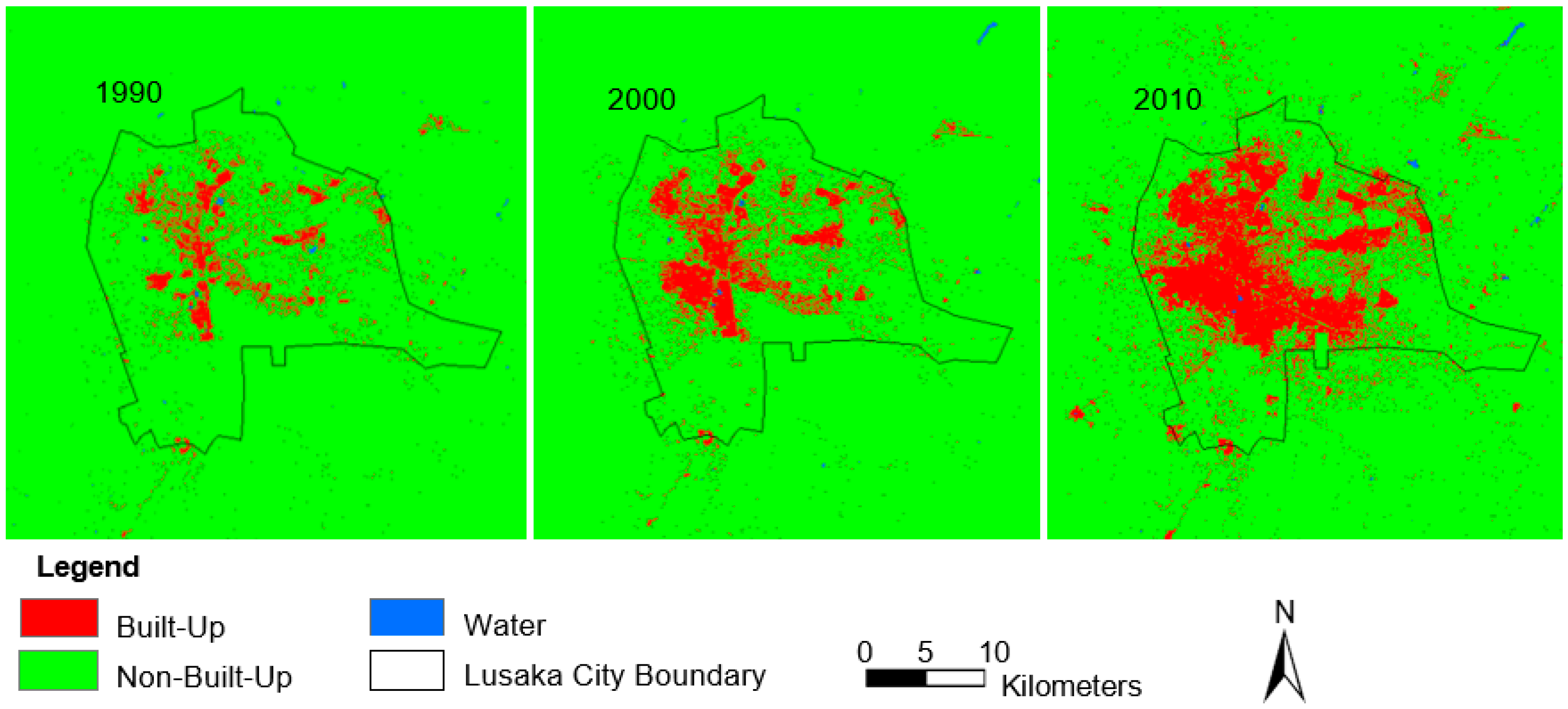
4.1. LUC Classification and Built-Area Extraction
4.2. ULU Classification
4.2.1. Accuracy Assessment and Hypothesis Validation
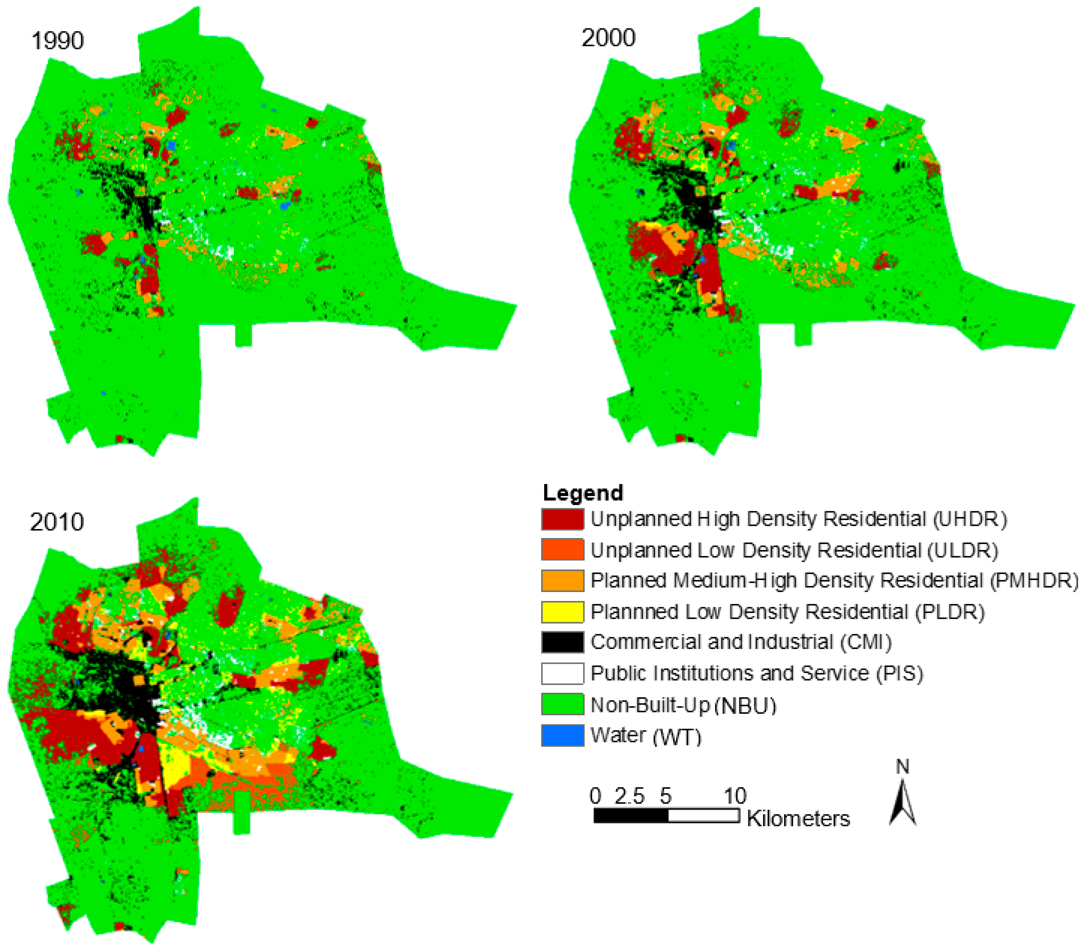
4.2.2. ULU Maps and Statistics
5. Discussion
5.1. Performance of ULU Classification Approach
5.2. Issues Related to the ULU Classification Approach
6. Conclusions
Acknowledgments
Author Contributions
Conflicts of Interest
References
- Barnsley, M.J.; Barr, S.L.; Hamid, A.; Muller, P.A.L.; Sadler, G.J.; Shepherd, J. Analytical tools to monitor urban areas. In Geographical Information Handling—Research and Applications; Mather, P.M., Ed.; John Wiley and Sons: Hoboken, NJ, USA, 1993; pp. 147–184. [Google Scholar]
- Herold, M.; Scepan, J.; Clarke, K.C. The use of remote sensing and landscape metrics to describe structures and changes in urban land uses. Environ. Plan. A 2002, 34, 1443–1458. [Google Scholar] [CrossRef]
- Stoler, J.; Daniels, D.; Weeks, J.R.; Stow, D.A.; Coulter, L.L.; Finch, B.K. Assessing the utility of satellite imagery with differing spatial resolutions for deriving proxy measures of slum presence in Accra, Ghana. GISci. Remote Sens. 2012, 1, 31–52. [Google Scholar] [CrossRef] [PubMed]
- Barnsley, M.J.; Barr, S.L. Inferring urban land use from satellite sensor images using kernel-based spatial reclassification. Photogramm. Eng. Remote Sens. 1996, 62, 949–958. [Google Scholar]
- Feyisa, G.L.; Meilby, H.; Darrel Jenerette, G.; Pauliet, S. Locally optimized separability enhancement indices for urban land cover mapping: Exploring thermal environmental consequences of rapid urbanization in Addis Ababa, Ethiopia. Remote Sens. Environ. 2016, 175, 14–31. [Google Scholar] [CrossRef]
- Shaba, M.A.; Dikshit, O. Improvement of classification in urban areas by the use of textural features: The case study of Lucknow city, Uttar Pradesh. Int. J. Remote Sens. 2001, 22, 565–593. [Google Scholar] [CrossRef]
- Myint, S.W.; Gober, P.; Brazel, A.; Grossman-Clarke, S.; Weng, Q. Per-pixel vs. object-based classification of urban land cover extraction using high spatial resolution imagery. Remote Sens. Environ. 2011, 115, 1145–1161. [Google Scholar] [CrossRef]
- Salehi, M.; Sahebi, M.R.; Maghsoudi, Y. Improving the accuracy of urban land cover classification using Radarsat-2 PolSAR data. IEEE J. Sel. Top. Appl. Earth Obs. Remote Sens. 2014, 7, 1394–1401. [Google Scholar]
- Harris, P.M.; Ventura, S.J. The integration of geographic data with remotely sensed imagery to improve classification in an urban area. Photogramm. Eng. Remote Sens. 1995, 61, 993–998. [Google Scholar]
- Hu, T.; Yang, J.; Li, X.; Gong, P. Mapping Urban Land Use by using Landsat Images and Open Social Data. Remote Sens. 2016, 8, 151. [Google Scholar] [CrossRef]
- Mesev, V. The use of census data in urban image classification. Photogramm. Eng. Remote Sens. 1998, 64, 431–436. [Google Scholar]
- Lu, D.; Weng, Q. Use of impervious surface in urban land-use classification. Remote Sens. Environ. 2006, 102, 146–160. [Google Scholar] [CrossRef]
- Mundia, C.N.; Aniya, M. Analysis of land use/cover changes and urban expansion of Nairobi city using remote sensing and GIS. Int. J. Remote Sens. 2005, 26, 2831–2849. [Google Scholar] [CrossRef]
- Kamusoko, C.; Gamba, J.; Murakami, H. Monitoring urban spatial growth in Harare Metropolitan. Adv. Remote Sens. 2013, 2, 322–331. [Google Scholar] [CrossRef]
- Gong, P.; Howarth, P.J. The Use of Structural Information for Improving Land-Cover Classification Accuracies at the Rural-Urban Fringe. Photogramm. Eng. Remote Sens. 1990, 56, 67–73. [Google Scholar]
- Steinnocher, K. Integration of Spectral and Spatial Classification Methods for Building a Land-Use Model of Austria. Int. Arch. Photogramm. Remote Sens. 1996, 31, 841–846. [Google Scholar]
- Van de Voorde, T.; Jacquet, W.; Canters, F. Mapping form and function in urban areas: An approach based on urban metrics and continuous impervious surface data. Landsc. Urban Plan. 2011, 102, 143–155. [Google Scholar] [CrossRef]
- Lu, D.; Weng, Q. Spectral mixture analysis of the urban landscape in Indianapolis with Landsat ETM+ imagery. Photogramm. Eng. Remote Sens. 2004, 70, 1053–1062. [Google Scholar] [CrossRef]
- Jensen, J.; Cowen, D. Remote sensing of urban suburban infrastructure and socio-economic attributes. Photogramm. Eng. Remote Sens. 1999, 65, 611–622. [Google Scholar]
- Mudau, N.; Mhangara, P.; Gebreslasie, M. Monitoring urban growth around Rustenburg, South Africa, using SPOT 5. S. Afr. J. Geomat. 2014, 3, 185–196. [Google Scholar] [CrossRef]
- Central Statistical Office (CSO). 2010 Census of Population and Housing; Lusaka, Zambia, 2012. Available online: http://www.zamstats.gov.zm/report/Census/2010/National/2010%20Census%20of%20Population%20Summary%20Report.pdf (accessed on 20 January 2017).
- Bhaskaran, S.; Paramananda, S.; Ramnarayan, M. Per-pixel and object-oriented classification methods for mapping urban features using Ikonos satellite data. Appl. Geogr. 2010, 30, 650–665. [Google Scholar] [CrossRef]
- Aguirre-Gutiérrez, J.; Seijmonsbergen, A.C.; Duivenvoorden, J.F. Optimizing land cover classification accuracy for change detection, a combined pixel-based and object-based approach in a mountainous area in Mexico. Appl. Geogr. 2012, 34, 29–37. [Google Scholar] [CrossRef]
- Li, X.; Meng, Q.; Gu, X.; Jancso, T.; Yu, T.; Wang, K.; Mavromatis, S. A hybrid method combining pixel-based and object-oriented methods and its application in Hungary using Chinese HJ-1 satellite images. Int. J. Remote Sens. 2013, 34, 4655–4668. [Google Scholar] [CrossRef]
- Trimble. eCognition® Developer 9.0 User Guide, 2014. Available online: http://www.eCognition.com/ (accessed on 22 February 2015).
- El-Kawy, O.A.; Rød, J.K.; Ismail, H.A.; Suliman, A.S. Land use and land cover change detection in the western Nile delta of Egypt using remote sensing data. Appl. Geogr. 2011, 31, 483–494. [Google Scholar] [CrossRef]
- Congalton, R.G. A review of assessing the accuracy of classification of remotely sensed data. Remote Sens. Environ. 1991, 37, 34–46. [Google Scholar] [CrossRef]
- Stefanov, W.L.; Ramsey, M.S.; Christensen, P.R. Monitoring urban land cover change: An expert system approach to land cover classification of semiarid to arid urban centers. Remote Sens. Environ. 2001, 77, 173–185. [Google Scholar] [CrossRef]
- Hung, M.; Ridd, M.K. A subpixel classifier for urban land-cover mapping based on a maximum-li kelihood approach and expert system rules. Photogramm. Eng. Remote Sens. 2002, 68, 1173–1180. [Google Scholar]
- Kahya, O.; Bayram, B.; Reis, S. Land cover classification with an expert system approach using Landsat ETM imagery: A case study of Trabzon. Environ. Monit. Assess. 2010, 160, 431–438. [Google Scholar] [CrossRef] [PubMed]
- Liu, X.; Long, Y. Automated identification and characterization of parcels with OpenStreetMap and points of interest. Environ. Plan. B Plan. Des. 2016, 43, 341–360. [Google Scholar] [CrossRef]
- Anderson, J.R.; Hardy, E.E.; Roach, J.T.; Witmer, R.E. A Land Use and Land Cover Classification System for Use with Remote Sensor Data; Geological Survey Professional Paper; USGS: Reston, VA, USA, 1976. [Google Scholar]
- Pontius, R.G., Jr.; Malizia, N.R. Effect of Category Aggregation on Map Comparison. Geogr. Inf. Sci. 2004, 3234, 251–268. [Google Scholar]
- Rocha, J.; Sousa, P.M.; Tenedório, J.A.; Encarnação, S. Land use/cover maps by RS and ancillary data integration in a GIS environment. Global developments in environmental earth orbservation from space. In Proceedings of the 25th EARSeL Symposium, Porto, Portugal, 6–11 June 2005; pp. 487–494. [Google Scholar]
- Chang, C.; Ye, Z.; Huang, Q.; Wang, C. An integrative method for mapping urban land use change using geo-sensor data. In Proceedings of the 1st International ACM SIGSPATIAL Workshop on Smart Cities and Urban Analytics, Seattle, WA, USA, 3–6 November 2015; pp. 47–54. [Google Scholar]
- Ghorbani, A.; Pakravan, M. Land use mapping using visual vs. digital image interpretation of TM and Google Earth derived imagery in Shrivan-Darasi watershed (Northwest of Iran). Eur. J. Exp. Biol. 2013, 3, 576–582. [Google Scholar]
- Jaafari, S.; Nazarisamani, A. Comparison between land use/land cover mapping through Landsat and Google Earth imagery. Am. J. Agric. Environ. Sci. 2013, 13, 763–768. [Google Scholar]
- Jacobson, A.; Cattau, M.; Riggio, J.; Petracca, L.; Fedak, D. Distribution and abundance of lions in northwest Tete Province, Mozambique. Trop. Conserv. Sci. 2013, 6, 87–107. [Google Scholar] [CrossRef]
- Jacobson, A.; Dhanota, J.; Godfrey, J.; Jacobson, H.; Rossman, Z.; Stanish, A.; Walker, H.; Riggio, J. A novel approach to mapping land conversion using Google Earth with an application to East Africa. Environ. Model. Softw. 2015, 72, 1–9. [Google Scholar] [CrossRef]
- Herold, M.; Liu, X.; Clarke, K.C. Spatial Metrics and Image Texture for Mapping Urban Land Use. Photogramm. Eng. Remote Sens. 2003, 69, 991–1001. [Google Scholar] [CrossRef]
- King, R.B. Land cover mapping principles: A return to interpretation fundamentals. Int. J. Remote Sens. 2002, 23, 3525–3545. [Google Scholar] [CrossRef]
- Puig, C.J.; Hyman, G.; Bolaños, S. Digital Classification vs. Visual Interpretation: A case study in humid tropical forests of the Peruvian Amazon. Int. Cent. Trop. Agric. 2002. Available online: https://www.researchgate.net/publication/237021820_Digital_Classification_vs_Visual_Interpretation_a_case_study_in_humid_tropical_forests_of_the_Peruvian_Amazon (accessed on 28 March 2017).


| Urban Land Use Class | Code | Description |
|---|---|---|
| Unplanned High Density Residential | UHDR | Residential areas (RD1 > 2,000 du/km2) comprising informal/slum/squatter settlements with many small houses located close to each other showing an enormously unsystematic spatial arrangement. Average RD was estimated at 5000 du/km2 and PD2 at 12,000–28,000 people/km2 |
| Unplanned3 Low Density Residential | ULDR | Residential areas (RD ≤ 2000 du/km2) comprising medium sized houses with slightly big lot sizes but showing a relatively unsystematic spatial arrangement. Average RD was estimated at 1500 du/km2 and PD at 400–2000 people/km2 |
| Planned4 Medium-High Density Residential | PHMDR | Residential areas (RD > 2000 du/km2) with many small and medium sized houses located close to each other showing a systematic spatial arrangement. Average RD was estimated at 3000 du/km2 and PD at 2000–22,000 people/km2 |
| Planned Low Density Residential | PLDR | Residential areas (RD ≤ 2000 du/km2) comprising large houses with big lot sizes and showing a systematic spatial arrangement. Average RD was estimated at 1000 du/km2 and PD at 400–2000 people/km2 |
| Commercial and Industrial | CMI | Commercial: General retail, shopping malls, markets, hotels, financial services (banks), roads, rails, etc.Industrial: Manufacturing, warehousing, quarrying, mining facilities, and commercial agriculture facilities |
| Public Institutions and Service | PIS | Areas comprising education and health facilities, religious institutions, government and administration houses, municipal utilities, transportation terminals, aviation facilities, etc. |
| Non-Built-Up | NBU | All vegetated areas (forest and grassland), bare lands, and agriculture areas |
| Water | WT | Rivers, streams, dams, etc. |
| ULU Map | Classified Data | Reference Data | Total | UA (%) | |||||
|---|---|---|---|---|---|---|---|---|---|
| UHDR | ULDR | PMHDR | PLDR | CMI | PIS | ||||
| 2010 | UHDR | 186 | 0 | 17 | 0 | 0 | 0 | 203 | 91.63 |
| ULDR | 4 | 54 | 10 | 4 | 0 | 1 | 73 | 73.97 | |
| PMHDR | 21 | 5 | 99 | 11 | 0 | 2 | 138 | 71.74 | |
| PLDR | 0 | 8 | 8 | 63 | 1 | 0 | 80 | 78.75 | |
| CMI | 0 | 0 | 0 | 3 | 127 | 2 | 132 | 96.21 | |
| PIS | 0 | 0 | 0 | 6 | 5 | 42 | 53 | 79.25 | |
| Total | 211 | 67 | 134 | 87 | 133 | 47 | 679 | ||
| PA (%) | 88.15 | 80.60 | 73.88 | 72.41 | 95.49 | 89.36 | |||
| Overall Classification Accuracy = 84.09%, Overall Kappa Coefficient = 80.63% | |||||||||
| 2000 | UHDR | 151 | 4 | 7 | 1 | 0 | 0 | 163 | 92.64 |
| ULDR | 2 | 26 | 0 | 0 | 0 | 0 | 28 | 92.86 | |
| PMHDR | 18 | 5 | 112 | 4 | 0 | 0 | 139 | 80.58 | |
| PLDR | 0 | 0 | 9 | 37 | 4 | 2 | 52 | 71.15 | |
| CMI | 0 | 0 | 5 | 0 | 85 | 1 | 91 | 93.41 | |
| PIS | 0 | 0 | 5 | 2 | 3 | 26 | 36 | 72.22 | |
| Total | 171 | 35 | 138 | 44 | 92 | 29 | 509 | ||
| PA (%) | 88.30 | 74.29 | 81.16 | 84.09 | 92.39 | 89.66 | |||
| Overall Classification Accuracy = 85.86%, Overall Kappa Coefficient = 84.02% | |||||||||
| ULU Class | 1990 | 2000 | 2010 | |||
|---|---|---|---|---|---|---|
| Area (Km2) | % | Area (Km2) | % | Area (Km2) | % | |
| UHDR | 13.85 | 3.32 | 25.26 | 6.05 | 46.88 | 11.22 |
| ULDR | 0.99 | 0.24 | 2.31 | 0.55 | 15.89 | 3.80 |
| PMHDR | 14.18 | 3.40 | 21.96 | 5.26 | 32.17 | 7.70 |
| PLDR | 4.77 | 1.14 | 9.00 | 2.16 | 20.61 | 4.93 |
| CMI | 11.20 | 2.68 | 19.31 | 4.62 | 33.65 | 8.06 |
| PIS | 4.18 | 1.00 | 6.32 | 1.51 | 9.61 | 2.30 |
| NBU | 367.36 | 87.95 | 333.11 | 79.75 | 258.47 | 61.88 |
| WT | 1.16 | 0.28 | 0.52 | 0.12 | 0.41 | 0.10 |
| Total | 418 | 100 | 418 | 100 | 418 | 100 |
© 2017 by the authors. Licensee MDPI, Basel, Switzerland. This article is an open access article distributed under the terms and conditions of the Creative Commons Attribution (CC BY) license (http://creativecommons.org/licenses/by/4.0/).
Share and Cite
Simwanda, M.; Murayama, Y. Integrating Geospatial Techniques for Urban Land Use Classification in the Developing Sub-Saharan African City of Lusaka, Zambia. ISPRS Int. J. Geo-Inf. 2017, 6, 102. https://doi.org/10.3390/ijgi6040102
Simwanda M, Murayama Y. Integrating Geospatial Techniques for Urban Land Use Classification in the Developing Sub-Saharan African City of Lusaka, Zambia. ISPRS International Journal of Geo-Information. 2017; 6(4):102. https://doi.org/10.3390/ijgi6040102
Chicago/Turabian StyleSimwanda, Matamyo, and Yuji Murayama. 2017. "Integrating Geospatial Techniques for Urban Land Use Classification in the Developing Sub-Saharan African City of Lusaka, Zambia" ISPRS International Journal of Geo-Information 6, no. 4: 102. https://doi.org/10.3390/ijgi6040102