Validation of Spatial Prediction Models for Landslide Susceptibility Mapping by Considering Structural Similarity


1
Institute of Geology and Geophysics, Chinese Academy of Sciences, Beijing 100029, China
2
University of Chinese Academy of Sciences, Beijing 100049, China
*
Authors to whom correspondence should be addressed.
ISPRS Int. J. Geo-Inf. 2017, 6(4), 103; https://doi.org/10.3390/ijgi6040103
Submission received: 5 January 2017
/
Revised: 7 March 2017
/
Accepted: 22 March 2017
/
Published: 30 March 2017
Abstract
:In this paper, we propose a methodology for validating landslide susceptibility results in the Pinggu district (Beijing, China). A landslide inventory including 169 landslides was prepared, and eight factors correlated to landslides (lithology, tectonic faults, topographic elevation, slope gradient, aspect, slope curvature, land use, and road network) were processed, integrating two techniques, namely the frequency ratio (FR) and the certainty factor (CF), in a geographic information system (GIS) environment. The area under the curve (success rate curve and prediction curve) analysis was used to evaluate model compatibility and predictability. Validation results indicated that the values of the area under the curve for the FR model and the CF model were 0.769 and 0.768, respectively. Considering spatial correlation, an alternative complementary method for validating landslide susceptibility maps was introduced. The spatially approximate maps could be discriminated from their matrices which carry structural information, and the structural similarity index (SSI) was then proposed to quantify the similarity. As a specific example, the SSI value of the FR (74.15%) scored higher than that of the CF model (69.36%), demonstrating its promise in validating different landslide susceptibility maps. These results show that the FR model outperforms the CF model in producing a landslide susceptibility map in the study area.
1. Introduction
Landslides are referred to as geological events involving the down-slope transport of soil/rock materials, and assessing their susceptibility constitutes a major task for local authorities to plan land use and mitigation [1,2]. Landslide susceptibility mapping (LSM) has been acknowledged as an effective tool to understand landslides and predict landslide-prone areas [3], and it addresses the propensity of soil/rock to produce various types of landslides, with susceptibilities expressed cartographically in maps that highlight the spatial distribution of potential slope-failure susceptibility [4].
Due to the complex nature of landslides, such as soil conditions, root strength, bedrock, topography, hydrology, and human activities, producing a reliable spatial prediction of landslides is still a challenging task. The best landslide model depends not only on the quality of the data used [5], but also strongly on the employed modeling approaches [6]. Nevertheless, the analysis of cause and consequence relationships is not always simple and, on many occasions, LSM has attracted heavy criticism [7]. For example, the geographic information system (GIS)-based interrelation analysis usually begins with the collection of landslide inventory maps, which mainly come from aerial photo-interpretation and systematic field checks [8,9]. The scale of the available aerial photographs, the topographic maps, the typology of the landslide phenomena, and the environmental contexts greatly affect the reliability and completeness of the landslide inventory map [10,11]. In addition, spatial resolution and pixel size effects [12,13], selection of conditional factors [14], criteria to classify each conditional factor map [15], and factor weight assignment techniques [16,17] also introduce uncertainties in LSM.
In GIS, if we consider a spatial database containing maps of lithological units, of land cover units, of topographic elevation and derived attributes (slope, aspect, etc.), and of the distribution in space of clearly identified mass movement, we can transform the multi-layered database into an aggregation of functional values to obtain an index of propensity of the land to failure [18]. For minimizing the subjectivity and bias in the weight assignment process, quantitative methods, such as statistical analysis [19] and deterministic analysis [20], may be utilized. The core issue then arises regarding the validation of the results of these models. Generally, validation can best be performed using the random-partition, spatial-partition, and time-partition techniques [21,22]. The time-partition technique enables validation to be performed by comparing landslides that occurred in a certain period and those that occurred in a different period, which is the most adequate to confirm the validity of the “prediction” made, but also the most difficult to apply as it requires the knowledge of the temporal distribution of landslides during a sufficiently long time span [23]. By employing mathematical statistics theory, various validation strategies have been introduced, which can be categorized as landslide density analysis [24], receiver operating characteristics (ROC) curve analysis, the area under ROC curve (AUC) analysis [25,26], and success rate or prediction rate curve analysis [26,27]. The landslide density analysis falsely assumes that landslide occurrence is a spatially continuous variable, and therefore it cannot be interpolated without considering the relation between landslide occurrence and the local geological settings [28]. The AUC computed from the ROC curve validates the accuracy of a landslide model in two aspects: prediction skill and model fitting [29]. When we exploit an inventory which was unknown in the model calibration, a predictive value is expected. When, instead of an independent population, the same landslide set is used, what is determined is how well the model fits the data. Similarly, the success rate method uses the training landslide pixels that have already been used for building the landslide models; thus, it is not suitable for assessing the prediction capacity of the models [30]. In the literature, the use of confusion matrix analysis [31] and agreed area analysis [32] were also reported for model validation. Despite much research effort towards LSM, there still remains a dispute on which method or technique is the best for the prediction of landslide-prone areas [33].
The main objective of this study is, therefore, to deal with the issue of validating landslide susceptibility models. Traditional validation methods (i.e., success rate curve analysis and prediction rate curve analysis) were firstly conducted to confirm the compatibility and predictive capacity of the landslide susceptibility models. Under such a premise, we proposed a validation approach based on the definition of a structural similarity index (SSI), which has the aim of discriminating the similarity between different landslide susceptibility models. The SSI seems to be effective to confirm the validity of the results of some models over other ones. An application example is presented to describe the strategy in this research and to provide a basis for generalizing the approach to validation.
2. Description of the Study Area
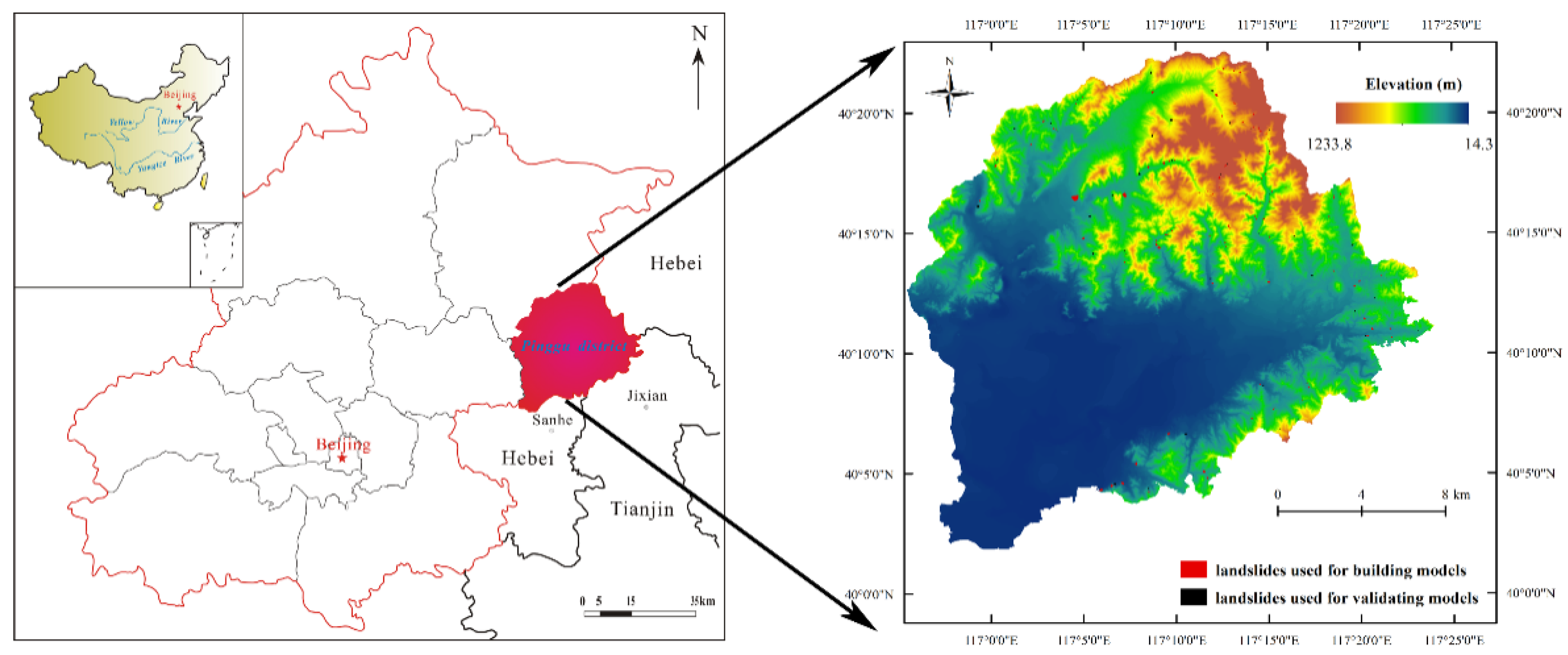
The study area (Figure 1) is about 1075 km2 and covers the whole area of the Pinggu district. It is located in the northeast of Beijing, China, between longitudes 116°55′ E and 117°25′ E, and latitudes 40°00′ N and 40°25′ N. The geomorphology is dominated by hilly and alluvial-proluvial landforms, with the elevation ranging from 14.3 m to 1233.8 m above sea level. The area experiences a continental monsoon climate, with uneven distribution of seasonal precipitation. According to the Beijing Meteorological Service, the annual average precipitation is 639.5 mm, and the rainy season commences in June and ends in September, with the heaviest precipitation during July, accounting for 74.9% of the yearly precipitation (recorded from 1981 to 2012, provided by the Pinggu weather station of the Beijing Meteorological Service).
Based on the geological map prepared by the Beijing Geological and Mineral Bureau [34], there are Archaeozoic metamorphic units, Proterozoic sedimentary units, and Quaternary deposit units in the area. Outcrops of Proterozoic sedimentary rocks are spread widely in the area, with the lithology of dolomites, dolomitic sandstones, and sandstones. Generally, road construction in mountainous areas cuts through these carbonatite rocks, and excavation of rock slopes during residence construction also leads to potential instability problems.
Due to the specific morphological settings, geology, and climate, landslides (especially rockfalls) are frequent in the area. A detailed site investigation was conducted, and geological and geotechnical studies were conducted on the landslides to gain a better understanding of the triggering mechanisms and failure processes and to better prepare for future failures in the study area. The main triggering factors are lithology and tectonic structures. Among the registered 169 landslides, 155 landslides were found, which are controlled by the altitude of discontinuities in the dolomitic sedimentary rocks. Ninety-six landslides were located on steep slopes (slope angle > 80°). Human activities (mainly land cover changes and road construction) also play an important role in landslide occurrence, as they increase the sensitivities of the surface layer to the effects of detachments/sliding. These events are destructive to roads (Figure 2), agricultural lands, and buildings.
3. Data and Materials
3.1. Landslide Inventory
The first important step in LSM is to identify landslide locations that occurred in the past and present [35]. In the area, slope movements are frequent, and over 70% of those movements are rockfalls. The landslide inventory was carried out to perform the analysis on a homogeneous population, and only one type of movement was selected: rockfalls. A detailed and reliable landslide inventory (Figure 1) map was prepared from two main sources: (1) the landslide database from aerial photograph (1:50,000) interpretation (obtained on 30 September 2012) with 16 landslide locations, and (2) detailed regional field investigation at 1:10,000 scale (undertaken from January to May 2013) with 153 landslide locations. A total of 169 landslides that have occurred during the last 20 years were registered. Figure 2 depicts the typical landslides observed during the field investigation.
In GIS, point data can be described as a singular (X,Y) coordinate, which does not reflect landslide affected areas, as this type of feature is usually used when the areal extent of a small landslide cannot be drawn due to the scale of the map [36]. However, the logical method is to reveal the landslide-responsible pixels. Lee et al. [37] suggested that when the scale of the map was 1:5000–1:50,000, the 5 m, 10 m, and 30 m pixel sizes yield similar accuracy. In this study, a pixel size of 30 m × 30 m was adopted, and landslides larger than one cell size were used for the analyses. For each landslide, the areal extent was delimited from the accumulation/depletion zone as a polygon feature drawn from field works, and converted to raster format in GIS.
3.2. Conditional Factors
Generally, the selection of landslide correlated factors should take the geologic characteristics of the study area and data availability into consideration. In GIS-based analysis, the selected factors should be operational, complete, non-uniform, measurable, and non-redundant [10]. For rockfall susceptibility mapping, Antoniou and Lekkas [38] indicated that geological information (e.g., discontinuities, joints and fault) and geomorphological information (e.g., slope angle and slope aspect) should be used as input parameters. In this study, eight conditional factors were recognized as correlated to rockfalls, i.e., lithology, proximity to major faults and road networks, slope degree, slope aspect, slope curvature, topographical elevation, and land cover were obtained (Figure 3). All of the above factors and landslides were then entered into the GIS medium using ArcGIS 10.1 software. The process of converting these continuous variables into categorical classes were conducted using expert opinions [39] and Jenks [40] natural breaks to define class intervals.
Lithology is considered as one of the most important factor because it influences the geomechanical characteristics of terrain (e.g., static and dynamic friction, restitution characteristics and fragmentation ratio), therefore controlling the types and mechanism of rockfalls [41]. The lithology map was constructed based on the geological mineral resources maps at 1:200,000 scale. This is the only geological map available for the study area. The lithology maps were constructed with nine lithological units, with their descriptions set out in Table 1.
Large-scale structures such as faults or thrusts induce regional perturbations in the fracturing occurrence and density, which are very unfavorable to natural or manmade slopes. The dip/dip direction often indicates the potential type of rockfalls [42]. In this study, the map of the distance to faults with eight classes was prepared.
A digital elevation model (DEM) for the study area with a spatial resolution of 30 m × 30 m was generated from topographic maps at a scale of 1:10,000. Based on the DEM, topographic attributes, such as slope, aspect, curvature, and elevation can be derived. It is well known that slope failures occur more readily on steeper slopes due to gravity stresses, since steeper slopes present a higher potential for failure, the materials that make up such slopes with steep angle can be expected to be stronger [38]. Geometric relationship between rock beds and slope aspect can influence the condition of ground water flow, and hence, the process and types of rockfall [43]. In general, if rocks are dipping in the same direction as the topographic surface, the slope is said to be cataclinal. If the beds dip in the direction opposite to the latter, anaclinal-slopes are created. When the strike of rock beds is perpendicular to the azimuth of mountain faces, the outcome are orthoclinal-slopes. As for slope curvature, it acts as major contributor to terrain instability in the way that it influence the concentration of the soil/rock moisture [44] and therefore influencing rockfalls. Though elevation by itself is not a conditional factor, there are some altitude ranges where the slope failures are frequent [32]. In this study, the four factors were constructed based on the DEM data: the slope map with eight classes, the aspect map with eight classes, the curvature map with eight classes, and the topographic elevation map with eight classes.
Land cover is also considered as indirect factor influencing rockfalls, for different land cover type in the slopes lead to different slope roughness and energy loss at impact [32]. Generally, NDVI (the normalized difference vegetation index) was used to measure surface reflectance and gives a quantitative estimate of the vegetation growth and biomass [36]. NDVI value was calculated by the formula:
where refers to the infrared portion of the electromagnetic spectrum, and is the red portion of the electromagnetic spectrum [45]. The NDVI map with six classes was then constructed based on the computed values.
The presence of the road is the major long-term factor affecting the stability of the rock mass. At the time of construction of the road, the buttress of the compartment was reduced and consequently, stresses increased in its base [43]. For this reason, road networks are included in GIS-based rockfall susceptibility analyses. In this study, distance to roads was proposed as an index to quantify this influence. Eight buffer categories were constructed.
4. Methodology
4.1. Preparation of Training and Validation Datasets
For landslide susceptibility modeling, landslide locations should be divided into training and validation datasets: the first one is used for building models and the other for validating models [46]. In this study, the specific dates of each landslide occurrence are mostly unknown; therefore, we randomly split these landslide locations into two subsets with a 7:3 ratio. The first is used for model construction, whereas the second is for model validation.
4.2. Landslide Susceptibility Modeling
Landslide susceptibility can be assessed using different methods based on GIS. Especially in the last 20 years, many research papers were published in order to solve the deficiencies and difficulties in the assessment of susceptibility. However, it should be noted that the procedure of preparing landslide susceptibility maps must be simple and must have a high accuracy. The frequency ratio model is one type of statistics-based approach widely used in landslide susceptibility analysis [36,47]. In the frequency ratio model, input processes, calculations, and output processes are very simple and can be readily understood. In addition, among the commonly used GIS analysis models for landslide susceptibility, the certainty factor has also been widely considered and experimentally investigated in the literature [48,49]. Therefore, in this study, the landslide susceptibility analyses were implemented using these two methods.
4.2.1. Frequency Ratio Method
The assumption that conditions leading to slope failure in the past and present are likely to cause landslides in the future is important for LSM [50]. Statistical approaches are based on the relationships between each landslide-related factor and the distribution of past landslides, and this correlation can be quantitatively evaluated using the frequency ratio (FR) model. The aforementioned eight landslide-correlated factors were used to establish this relationship with landslides.
The number of landslide pixels in each class has been evaluated and the frequency ratio for each factor class is found by dividing the landslide ratio by the area ratio [51], denoted as:
where is the frequency ratio of class in factor ; is the number of pixels of landslide occurrence within class in factor ; is the number of pixels of class in factor . In relation analyses, a value greater than 1.0 indicates a strong correlation between landslide occurrence and the factor’s class, and a value lower than 1.0 means a weak correlation [52]. Once the frequency ratio of each landslide factor’s class was obtained, the landslide susceptibility index (LSI) could be calculated by summation of each factor’s frequency ratio values. A higher LSI means a higher susceptibility to landslides while a lower LSI indicates a lower susceptibility to landslides [47].
4.2.2. Certainty Factor Method
The certainty factor (CF) is one of the possible proposed favorability functions to handle the problem of the combination of heterogeneous data. The CF is calculated for each data layer based on the landslide inventory and the landslide occurrence frequency in each class of every thematic layer. The CF for each pixel is defined as the change in certainty that a proposition is true from without the evidence (prior probability of having landslide in the study area) to be given the evidence (conditional probability of having a landslide given a certain class of a thematic layer) for each data layer [49]. The CF, as a function of probability, originally proposed by Shortliffe and Buchanan, [53] is:
where CF is the certainty factor, is the conditional probability of having a number of landslides in a class (e.g., south-facing slope in the aspect layer, Quaternary deposits in the lithology layer) and is the prior probability of having the total number of landslides in the study area. The CF ranges between –1 and 1, where positive values imply an increase in certainty, after the evidence of a landslide is observed, and negative values correspond to a decrease in certainty. A value close to 0 means that the prior probability is very similar to the conditional one, hence it does not give any indication about the certainty of the occurrence of the event [54].
The layers are combined pairwise according to the integration rules [55]. The combination of CF values of two thematic layers ‘z’ is expressed in the following equation given by Binaghi et al. [56]:
the CF values are computed by overlaying each thematic layer with the landslide inventory map and calculating the landslide frequencies. Each thematic layer is reclassified according to the CF value calculated and they are combined pairwise to obtain the LSI using the integration rule of the equation.
4.3. Model Validation Strategies
Validation implies a comparison between the maps obtained from the models and the independent dataset. This comparison can be qualitative—for example, visually, by a simple overlay—or quantitative, performed using functions such as the cumulative curve [22]. The current study attempts to analyze the spatial correlation between different landslide models, and to offer as an alternative a procedure which is based on the evaluation of the similarity between different methods. To realize this, traditional validation approaches, i.e., success rate and prediction rate curves, were firstly used for testing the model compatibility and prediction capacity. On such a premise, the spatially correlated validation was then performed to obtain the SSI, which can quantitatively validate the performance of different landslide models.
4.3.1. Traditional Validation Approaches
Landslide susceptibility maps can be verified by comparing the susceptibility maps with both the training data that were used for building the models with the validation data that were not used during the model building process.
The success rate curve is based on the comparison between the prediction image and the landslides used in the modeling [21], and the success rate method can help determine how well the resulting landslide susceptibility maps have classified the areas of existing landslides [30]. The prediction rate method mimics the comparison by partitioning landslide data; one subset of the data (training data) is used for obtaining a prediction image, and the other subset (validation data) is compared with the prediction results for validation, explaining how well the model and predictor variables predict the results [55]. In both techniques, the rate curves can be created. The area under the successive rate curve (AUSC) represents the quality of landslide models to reliably classify the occurrence of existing landslides (training dataset), while the area under the predicted rate curve (AUPC) explains the capacity of the proposed landslide model for predicting landslide susceptibility. The AUC value ranges from 0.5 to 1.0, and an ideal model has an AUC value close to 1.0 (perfect fit/prediction), whereas a random fit/prediction model has an AUC value close to 0.5 [57]. In this study, we use 10 subdivisions of LSI values of all cells in the study area, the cumulative percentage of landslide occurrence (the training dataset and validation dataset, respectively) in the classes was calculated, and curves were then drawn to calculate their AUCs.
4.3.2. Spatially Correlated Validation Approaches
When a landslide susceptibility map consists of different levels of susceptibility, we usually visualize such thematic representations. It should be noted that the prediction map is constructed using mathematical models by computing a predicted value at each pixel on a continuous scale, and pixel values from two prediction maps may have different meanings. For an objective and proper comparison of the prediction maps, the ranking of equal-number classes [55] is firstly used, i.e., all of the pixels are sorted according to the pixel values in descending order, and the total number of pixels is divided into a number of classes with an equal number of pixels.
For comparing prediction maps, a virtual standard map (VSM) is expected. The VSM is constructed based on the intersection of the compared maps, and it contains mutual pixels which correspond to the same susceptible level in the compared maps. For instance, if we rank the respective pixel values derived from two individual landslide models into four levels for visualization, two prediction maps can be interpreted and denoted as map A and B, and the pixels in the first class of the VSM are pixels in the first class of both map A and map B. Since both map A and map B should be firstly subjected to the same validation (success rate and prediction rate curve analysis) to confirm their compatibility and validity, the reliability of the VSM can be guaranteed.
In the result of landslide susceptibility maps, different landslide susceptibility classes can also be demonstrated at a discrete level; the grey level of every pixel is an integer between 0 and 255, and different grey levels represent different LSIs. Meanwhile, the visible landslide susceptibility maps can be regarded as natural images that are highly structured, which are exhibited by various positional combinations of pixels of different grey levels. In fact, the produced landslide susceptibility maps in GIS are intrinsically a matrix carrying structural information. Therefore, the structural information can be extracted from the spatially approximate maps to measure the similarity between two arbitrary maps.
To obtain the matrices of the maps, image processing techniques can be adopted to optimize the landslide susceptibility maps/images and extract edges by the grey level threshold based on the local entropy of the image in MATLAB. Suppose and are two matrices of the two prediction images which have been aligned with each other. If we consider one of the matrices to have perfect quality, i.e., the map from which this matrix is derived is more suitable and predictable, then the similarity measure can serve as a quantitative measurement of the quality of the second matrix. In this way, the spatial similarity of two landslide susceptibility maps can eventually be quantitatively evaluated by a structural similarity index (SSI) [58]. In mathematical form, the SSI is denoted as:
where , are the element in matrix , respectively. Using the matrix manipulation functions in MATLAB, the SSI can be easily obtained. The value of the SSI ranges from 0 to 1.0, with the explanation that the higher the SSI, the higher the similarity of the two matrices, i.e., the more approximately a landslide susceptibility map resembles the other.
In this study, the colorized landslide susceptibility maps were constructed based on the results of the FR and CF models, respectively. Then they were classified into four susceptibility classes (very low, low, moderate, and high susceptibility classes). Using the embedded functions in MATLAB, these colorized maps can be converted into grey figures. Through matrix manipulation functions in MATLAB, the SSI can be easily calculated according to Equation (5).
5. Results and Analysis
5.1. Landslide Conditional Factor Analysis
Using the aforementioned conditional factors, FR and CF were built using the training dataset. The result is set out in Table 2.
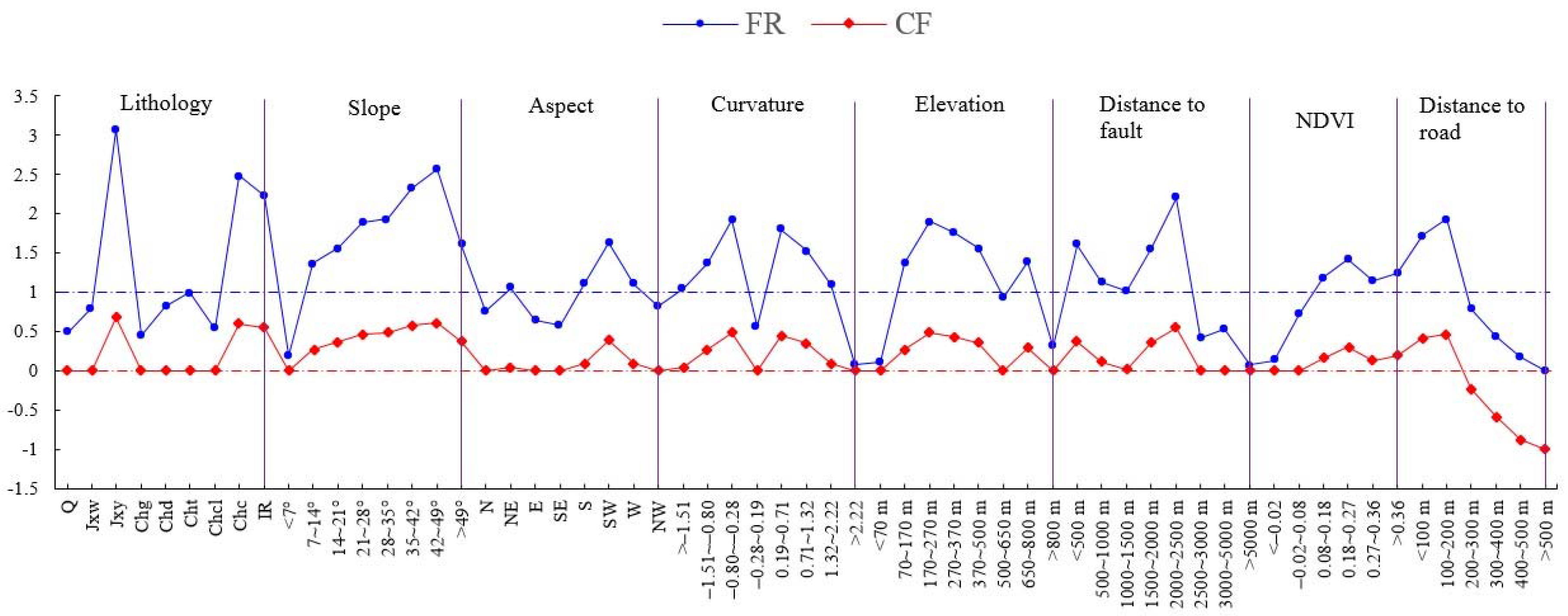
For comparison, the calculated and for each class/type of the conditional factors were plotted in Figure 4. It can be seen that the variations of are in consistent with those of . When the CF gives the degree of belief, the denotes the level of correlation between landslide locations and conditional factors. It was observed that the lithology factor is closely correlated to landslide occurrence, as most of the landslides have occurred in the class of Jxy, Chc, and IR. With the increase of the slope gradient, landslides are more likely to occur. Additionally, areas within 1500−2100 m from the road networks and those within 2000–2500 m from major faults have a higher probability for landslides to occur.
5.2. Model Results and Analysis
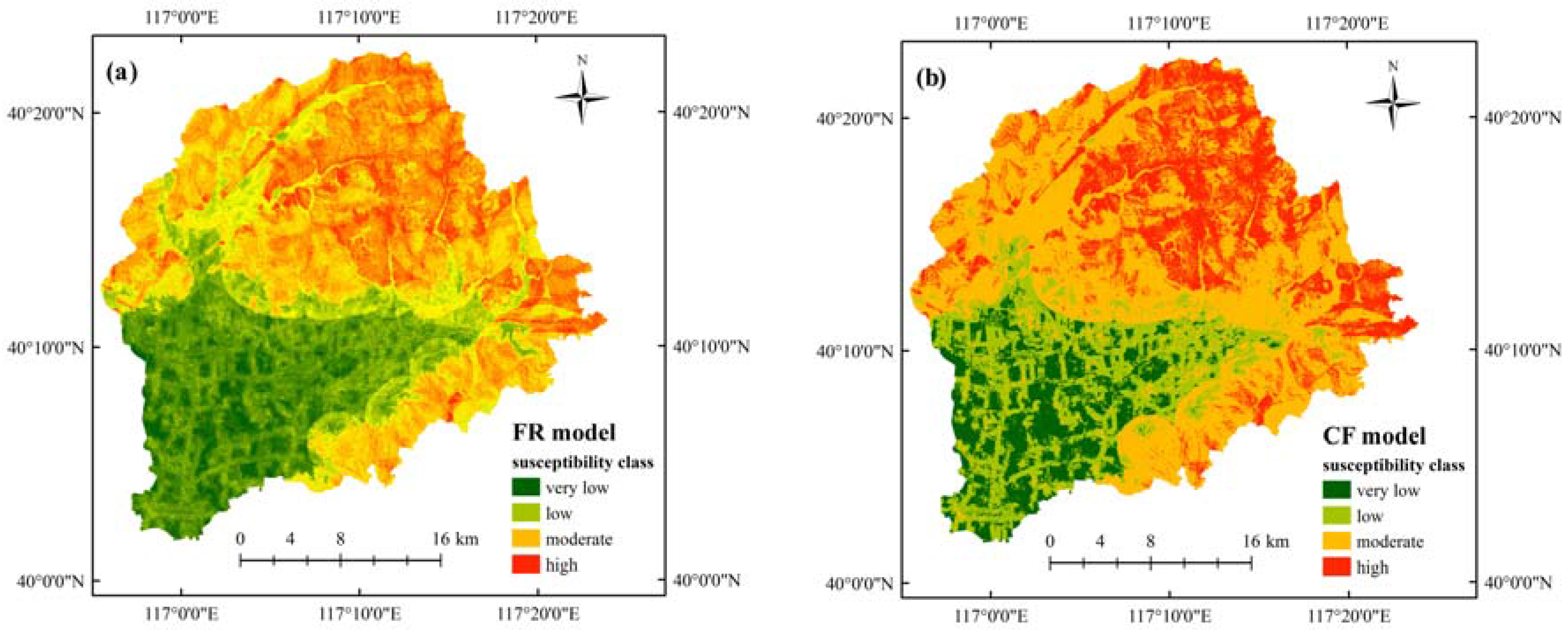
Once the FR and CF models were successfully trained in the training process, they were used to calculate the LSI for all pixels in the domain. LSIs were reclassified into four susceptibility levels as high, moderate, low, and very low, using the equal-number classes [18] method. For the purpose of visualization, the two landslide susceptibility maps produced from the FR and CF models are shown in Figure 5.
5.3. Model Validation and Comparison
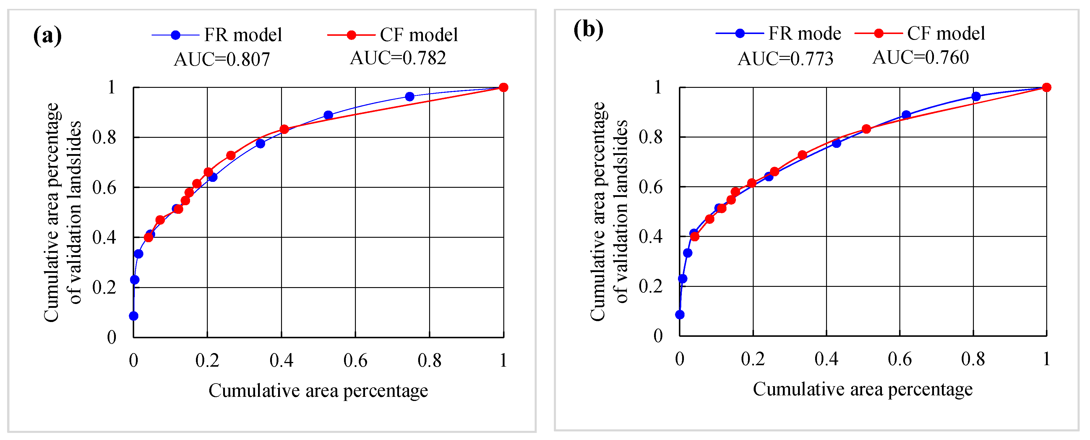
The compatibility of the susceptibility models was evaluated using the training dataset. Correspondingly, their prediction probability was assessed using the validating dataset. The area under the curve approach was used, and the results are shown in Figure 6. Respective AUC values of 0.807 and 0.773 for the FR model and the CF model showed that the map obtained from the FR model gives a higher accuracy in classifying the areas of existing landslides. For the prediction capacity evaluation of the developed landslide models, the prediction rate curve was obtained using the landslide pixels in the validating dataset (30% of the total observed landslides), and it can be seen from Figure 6 that both of the models have a good prediction capability, with the higher one for the FR model (AUC = 0.773), and the prediction capacities of the two models can be evaluated relatively similarly.
In the study, the VSM was generated from maps produced by the FR and CF models, and the matrix of the VSM was assigned to , while the matrices of maps derived from the FR and CF models were, respectively, assigned to . Using the image processing technique in MATLAB, the grey figures of the VSM and the landslide susceptibility maps produced by the FR and CF models were obtained. Based on Equation (5), a matrix manipulation function was adopted to calculate the SSIs. Calculation results showed that the SSIs between the matrices of the VSM and the map produced by the FR model, and the VSM and the map produced by CF model are 78.43% and 71.42%, respectively. This indicates that the landslide susceptibility map produced by the FR model yields the maximum approximation to the VSM.
Therefore, from the perspective of both model compatibility and predictability, the FR model slightly outperforms the CF model, but the difference in performance is slight, as represented by the AUCs. However, the SSI seems to amplify this difference, and the relative discrepancy becomes evident, so that it can confirm the validity of the results of the FR model over the CF model with much more confidence.
6. Discussion and Conclusions
Methodologies for producing landslide susceptibility maps are various, based on GIS technology, and much literature has been published in order to solve the deficiencies and difficulties in landslide susceptibility assessment. However, it should be noted that the procedure for preparing landslide susceptibility maps must be simple and must have a higher accuracy [36].
In this study, the frequency ratio model, as a simple method, and the certainty factor, as a complicated method, were applied to construct landslide susceptibility models. In the frequency ratio model, the input process, calculations, and output process are simple and can be readily understood [59]. However, the certainty factor involves vast calculations and complicated data processing, it requires conversions of data in raster format to shapefiles, and another conversion to raster format again after statistical analyses are completed, and these data, again, need complex logical calculations in GIS to obtain the final results.
For validating landslide susceptibility models (maps), Sarkar and Kanungo [60] stated that in an ideal landslide susceptibility map, the very high susceptible class should have the highest landslide density or area proportion, and there should be a decreasing trend in the landslide density and percentage of landslide area successively from very high to very low susceptible zones. As a result, in this study, higher accuracies of LSM for the two models were obtained. Using the training data, the respective AUC values for the FR and CF models were 0.807 and 0.773. When, instead of a training dataset, the validating dataset was used, the AUC values for the FR and CF models were 0.782 and 0.760, respectively. Swets [57] suggested that the AUC values between 0.7 and 0.9 indicate a reasonable discrimination ability. Thus, it could be evaluated that both of the models have a relatively similar partition performance and prediction ability. Taking the spatial discrepancies of the corresponding susceptible classes within each map, the spatially correlated validation method described here is shown to be useful while working on map validation. Therefore, the structural similarity can serve as a complementary validation approach for map comparison when traditional methods fail to confirm the validity of one model over others in a targeted place.
The FR and CF models quantitatively estimate landslide susceptibility given a set of geo-environmental conditions. In fact, the landslide disaster itself is a typical nonlinear system, and the relationship between various factors is complex; a susceptibility map of landslides based on any stochastic methods remains uncertain. However, rather than serving as the best landslide model, the FR model presents a better performance in producing landslide susceptibility map in the study area when compared to the CF model.
Acknowledgments
This study is finally supported by the National Natural Science Foundation of China (Nos. 41372322, 41172269) and the Key National Natural Science Foundation of China (No. 41330643). The authors would like to express their sincerest gratitude to the anonymous reviewers for their valuable and constructive comments.
Author Contributions
The three authors contributed equally to the present paper. Field investigation works were performed by Deng, Tan, under the supervision of Li. Deng and Li analyzed the data and wrote the paper. A general supervision was provided by Li. All authors have read and approved the final manuscript.
Conflicts of Interest
The authors declare no conflict of interest.
References
- Corominas, J.; van Westen, C.; Frattini, P.; Cascini, L.; Malet, J.P.; Fotopoulou, S.; Catani, F.; Van DenEeckhaut, M.; Marouli, O.; Agliardi, F.; et al. Recommendations for the quantitative analysis of landslide risk. Bull. Eng. Geol. Environ. 2014, 73, 209–263. [Google Scholar] [CrossRef]
- Ba, Q.Q.; Chen, Y.M.; Deng, S.S.; Wu, Q.J.; Yang, J.X.; Zhang, J.Y. An improved information value model based on gray clustering for landslide susceptibility mapping. ISPRS Int. J. Geo-Inf. 2017, 6, 18. [Google Scholar] [CrossRef]
- Feizizadeh, B.; Roodposhti, M.S.; Jankowski, P.; Blaschke, T. A GIS-based extended fuzzy multi-criteria evaluation for landslide susceptibility mapping. Comput. Geosci. 2014, 73, 208–221. [Google Scholar] [CrossRef] [PubMed]
- Feizizadeh, B.; Blaschke, T.; Nazmfar, H.; Rezaei Moghaddam, M.H. Landslide susceptibility mapping for the Urmia Lake basin, Iran: A multi-criteria evaluation approach using GIS. Int. J. Environ. Res. 2013, 7, 319–336. [Google Scholar]
- Jebur, M.N.; Pradhan, B.; Tehrany, M.S. Optimization of landslide conditioning factors using very high-resolution airborne laser scanning (LiDAR) data at catchment scale. Remote Sens. Environ. 2014, 152, 150–165. [Google Scholar] [CrossRef]
- Tien Bui, D.; Tuan, T.A.; Klempe, H.; Pradhan, B.; Revhaug, I. Spatial prediction models for shallow landslide hazards: A comparative assessment of the efficacy of support vector machines, artificial neural networks, kernel logistic regression, and logistic modes tree. Landslides 2016, 13, 361–378. [Google Scholar] [CrossRef]
- Wang, X.L.; Zhang, L.Q.; Wang, S.J.; Lari, S. Regional landslide susceptibility zoning with considering the aggregation of landslide points and the weights of factors. Landslides 2014, 11, 399–409. [Google Scholar] [CrossRef]
- Ardizzone, F.; Cardinali, M.; Carrara, A.; Guzzetti, F.; Reichenbach, P. Impact of mapping errors on the reliability of landslide hazard maps. Nat. Hazards Earth Syst. 2002, 2, 3–14. [Google Scholar] [CrossRef]
- Conforti, M.; Muto, F.; Rago, V.; Critelli, S. Landslide inventory map of north-eastern Calabria (South Italy). J. Maps 2014, 10, 90–102. [Google Scholar] [CrossRef]
- Ayalew, L.; Yamagishi, H.; Maruib, H.; Kannoc, T. Landslides in Sado Island of Japan: Part II. GIS-based susceptibility mapping with comparisons of results from two methods and verification. Eng. Geol. 2005, 81, 432–445. [Google Scholar] [CrossRef]
- Galli, M.; Ardizzone, F.; Cardinali, M.; Guzzzetti, F.; Reichenbach, P. Comparing landslide inventory maps. Geomorphology 2008, 94, 268–289. [Google Scholar] [CrossRef]
- Vander Jagt, B.J.; Durand, M.T.; Margulis, S.A.; Kim, E.J.; Molotch, N.P. The effect of spatial variability on the sensitivity of passive microwave measurement to snow water equivalent. Remote Sens. Environ. 2013, 136, 163–179. [Google Scholar] [CrossRef]
- Chang, K.T.; Dou, J.; Chang, Y.; Liu, J.K. Spatial resolution effects of digital terrain models on landslide susceptibility analysis. ISPRS-Int. Arch. Photogramm. Remote Sens. Spat. Inf. Sci. 2016, XLI-B8, 33–36. [Google Scholar] [CrossRef]
- Meten, M.; PrakashBhandary, N.; Yatabe, R. Effect of landslide factor combinations on the prediction accuracy of landslide susceptibility maps in the Blue Nile Gorge of Central Ethiopia. Geoenviron. Disasters 2015, 2, 9. [Google Scholar] [CrossRef]
- Wang, L.J.; Sawada, K.; Moriguchi, S. Landslide susceptibility analysis using light detection and ranging-derived digital elevation models and logistic regression models: A case study in Mizunami City, Japan. J. Appl. Remote Sens. 2013, 7, 121–130. [Google Scholar] [CrossRef]
- Pradhan, B.; Lee, S. Landslide susceptibility assessment and factor effect analysis: Backpropagation artificial neural networks and their comparison with frequency ratio and bivariate logistic regression modelling. Environ. Model. Softw. 2010, 25, 747–759. [Google Scholar] [CrossRef]
- Akgun, A.; Sezer, E.A.; Nefeslioglu, H.A.; Gokceoglu, C.; Pradhan, B. An easy-to-use MATLAB program (MamLand) for the assessment of landslide susceptibility using a Mamdani fuzzy algorithm. Comput. Geosci. 2012, 38, 23–34. [Google Scholar] [CrossRef]
- Chung, C.J.; Fabbri, A.G. Probabilistic prediction models for landslide hazard mapping. Photogramm. Eng. Remote Sens. 1999, 65, 1389–1399. [Google Scholar]
- Pradhan, B.; Mansor, S.; Pirastech, S.; Buchroithner, M.F. Landslide hazard and risk analyses at a landslide prone catchment area using statistical based geospatial model. Int. J. Remote Sens. 2011, 32, 4075–4087. [Google Scholar] [CrossRef]
- Thanh, L.; De Smedt, F. Slope stability analysis using a physically based model: A case study from a Luoi district in Thua Thien-Hue province, Vietnam. Landslide 2014, 11, 897–907. [Google Scholar] [CrossRef]
- Chung, C.J.; Fabbri, A.G. Validation of spatial prediction models for landslide hazard mapping. Nat. Hazards 2003, 30, 451–472. [Google Scholar] [CrossRef]
- Remondo, J.; Gonzalez, A.; Diaz De Teran, J.R.; Cendrero, A.; Fabbri, A.; Chung, C.J. Validation of landslide susceptibility maps: Example and applications from a case study in Northern Spain. Nat. Hazards 2004, 30, 437–449. [Google Scholar] [CrossRef]
- Femandez, C.I.; Castillo, T.F.D.; Hamdouni, R.E.; Montero, J.C. Verification of landslide susceptibility mapping: A case study. Earth Surf. Landf. 1999, 24, 537–544. [Google Scholar] [CrossRef]
- Guzzetti, F.; Cardinali, M.; Reichenbach, P.; Carrara, A. Comparing landslide maps: A case study in the upper Tiber river basin, Central Italy. Environ. Manag. 2000, 25, 247–263. [Google Scholar] [CrossRef]
- Fawcett, T. An introduction to ROC analysis. Pattern Recogn. Lett. 2006, 27, 861–874. [Google Scholar] [CrossRef]
- Frattini, P.; Crosta, G.B.; Carrara, A. Techniques for evaluating the performance of landslide susceptibility models. Eng. Geol. 2010, 111, 62–72. [Google Scholar] [CrossRef]
- Mohammady, M.; Pourghasemi, H.R.; Pradhan, B. Landslide susceptibility mapping at Golestan Province, Iran: A comparison between frequency ratio, Dempster-Shafer, and weights-of-evidence models. J. Asian Earth Sci. 2012, 61, 221–236. [Google Scholar] [CrossRef]
- Aghdam, I.N.; Pradhan, B. Landslide susceptibility mapping using an ensemble statistical index (Wi) and adaptive neuro-fuzzy inference system (ANFIS) model at alborz mountains (Iran). Environ. Earth Sci. 2016, 75, 1–20. [Google Scholar] [CrossRef]
- Ozdemir, A.; Altural, T. A comparative study of frequency ratio, weights of evidence and logistic regression methods for landslide susceptibility mapping: Sultan Mountains, SW Turkey. J. Asian Earth Sci. 2013, 64, 180–197. [Google Scholar] [CrossRef]
- Tien Bui, D.; Pradhan, B.; Lofman, O.; Revhaug, I.; Dick, O.B. Spatial prediction of landslide hazards in Hoa Binh province (Vietnam): A comparative assessment of the efficacy of evidential belief functions and fuzzy logic models. Catena 2012, 96, 28–40. [Google Scholar] [CrossRef]
- Van Westen, C.J.; Rengers, N.; Soeters, R. Use of geomorphological information in indirect landslide susceptibility assessment. Nat. Hazards 2003, 30, 399–419. [Google Scholar] [CrossRef]
- Bijukchhen, S.M.; Kayastha, P.; Dhital, M.R. A compressive evaluation of heuristic and bivariate statistical modelling for landslide susceptibility mappings in Ghurmi-Dhad Khola, east Nepal. Arab. J. Geosci. 2013, 6, 2727–2743. [Google Scholar] [CrossRef]
- Dagdelender, G.; Nefeslioglu, H.A.; Gokceoglu, C. Landslide susceptibility model validation: A routine starting from landslide inventory to susceptibility. In Landslide Science for a Safer Geoenvironment; Sassa, K., Canuti, P., Yin, Y., Eds.; Springer: Cham, Switzerland, 2014. [Google Scholar]
- Beijing Geological and Mineral Bureau. The Expedition Report of Regional Geology Survey (Dahuashan Sheet, Pinggu Sheet, 1:50 000); Beijing Geological and Mineral Bureau: Beijing, China, 1995.
- Jimenez-Peralvarez, J.D.; Irigaray, C.; El Hamdouni, R.; Chacon, J. Landslide susceptibility mapping in a semi-arid mountain environment: An example from the southern slopes of Sierra Nevada (Granada, Spain). Bull. Eng. Geol. Environ. 2011, 70, 265–277. [Google Scholar] [CrossRef]
- Yilmaz, I. Landslide susceptibility mapping using frequency ratio, logistic regression, artificial neural networks and their comparison: A case study from Kat landslides (Tokat-Turkey). Comput. Geosci. 2009, 35, 1125–1138. [Google Scholar] [CrossRef]
- Lee, S.; Choi, J.; Woo, I. The effect of spatial resolution on the accuracy of landslide susceptibility mapping: A case study in Boun, Korea. Geosci. J. 2004, 8, 51–60. [Google Scholar] [CrossRef]
- Andreas, A.A.; Lekkas, E. Rockfall susceptibility map for Athinios port, Santorini Island, Greece. Geomorphology 2010, 118, 152–166. [Google Scholar]
- Tien Bui, D.; Lofman, O.; Revhaug, I.; Dick, O. Landslide susceptibility analysis in the Hoa Binh province of Vietnam using statistical index and logistic regression. Nat. Hazards 2011, 59, 1413–1444. [Google Scholar]
- Jenks, G.F. Generalization in statistical mapping. Ann. Assoc. Am. Geogr. 1963, 53, 15–26. [Google Scholar] [CrossRef]
- Tien Bui, D.; Ho, T.C.; Pradhan, B.; Pham, B.T.; Nhu, V.H.; Revhaug, I. GIS-based modeling of rainfall-induced landslides using data mining-based functional trees classifier with AdaBoost, Bagging, and MultiBoost ensemble frameworks. Environ. Earth Sci. 2016, 75, 1101. [Google Scholar] [CrossRef]
- Baillifard, F.; Jaboyedoff, M.; Sartori, M. Rockfall hazard mapping along a mountainous road in Switzerland using a GIS-based parameter rating approach. Nat. Hazards Earth Syst. Sci. 2003, 3, 431–438. [Google Scholar] [CrossRef]
- Ayalew, L.; Yamagishi, H. The application of GIS-based logistic regression for landslide susceptibility mapping in the Kakuda-Yahiko Mountains, Central Japan. Geomorphology 2005, 65, 15–31. [Google Scholar] [CrossRef]
- Yilmaz, C.; Topal, T.; Suzen, M.L. GIS-based landslide susceptibility mapping using bivariate statistical analysis in Devrek (Zonguldak-Turkey). Environ. Earth Sci. 2012, 65, 2161–2178. [Google Scholar] [CrossRef]
- Wu, Y.L.; Li, W.P.; Liu, P.; Bai, H.Y.; Wang, Q.Q.; He, J.H.; Liu, Y.; Sun, S.S. Application of analytic hierarchy process model for landslide susceptibility mapping in the Gangu County, Gansu Province, China. Environ. Earth Sci. 2016, 75, 1–11. [Google Scholar] [CrossRef]
- Chung, C.J.; Fabbri, A.G. Predicting landslides for risk analysis-spatial models tested by a cross-validation technique. Geomorphology 2008, 94, 438–452. [Google Scholar] [CrossRef]
- Lee, S.; Pradhan, B. Landslide hazard mapping at Selangor, Malaysia using frequency ratio and logistic regression models. Landslides 2007, 4, 33–41. [Google Scholar] [CrossRef]
- Pourghasemi, H.R.; Pradhan, B.; Gokceoglu, C.; Mohammadi, M.; Moradi, H.R. Application of weights-of-evidence and certainty factor models and their comparison in landslide susceptibility mapping at Haraz watershed, Iran. Arab. J. Geosci. 2013, 6, 2351–2365. [Google Scholar] [CrossRef]
- Sujatha, E.R.; Rajamanickam, G.V.; Kumaravel, P. Landslide susceptibility analysis using Probabilistic Certainty Factor Approach: A case study on Tevankarai stream watershed, India. J. Earth Syst. Sci. 2012, 121, 1337–1350. [Google Scholar] [CrossRef]
- Lee, S. Application of likelihood ratio and logistic regression model for landslide susceptibility mapping using GIS. Environ. Manag. 2004, 34, 223–232. [Google Scholar] [CrossRef]
- Lee, S.; Talib, J.A. Probabilistic landslide susceptibility and factor effect analysis. Environ. Geol. 2005, 47, 982–990. [Google Scholar] [CrossRef]
- Pradhan, B. Landslide susceptibility mapping of a catchment area using frequency ratio, fuzzy logic and multiple logistic regression approaches. J. Indian Soc. Remote Sens. 2010, 38, 301–320. [Google Scholar] [CrossRef]
- Shortliffe, E.H.; Buchanan, G.G. A model of inexact reasoning in medicine. Math. Biosci. 1975, 23, 351–379. [Google Scholar] [CrossRef]
- Pourghasemi, H.R.; Mohammady, M.; Pradhan, B. Landslide susceptibility mapping using index of entropy and conditional probability models in GIS: Safarood Basin, Iran. Catena 2012, 97, 71–84. [Google Scholar] [CrossRef]
- Chung, C.J.; Fabbri, A.G. The representation of geosciences information for data integration. Non-Renew. Resour. 1993, 2, 122–139. [Google Scholar] [CrossRef]
- Binaghi, E.; Luzi, L.; Madella, P. Slope instability zonation: A comparison between certainty factor and fuzzy Dempster–Shafer approaches. Nat. Hazards 1998, 17, 77–97. [Google Scholar] [CrossRef]
- Swets, J.A. Measuring the accuracy of diagnostic systems. Science 1988, 240, 1285–1293. [Google Scholar] [CrossRef] [PubMed]
- Wang, Z.; Bovik, A.C.; Sheikh, H.R.; Simoncelli, E.P. Image quality assessment: From error visibility to structural similarity. IEEE Trans. Image Process. 2004, 13, 600–612. [Google Scholar] [CrossRef] [PubMed]
- Lee, S.; Min, K. Statistical analyses of landslide susceptibility at Yongin, Korea. Environ. Geol. 2001, 40, 1095–1113. [Google Scholar] [CrossRef]
- Sarkar, S.; Kanungo, D.P. An integrated approach for landslide susceptibility mapping using remote sensing and GIS. Photogramm. Eng. Remote Sens. 2004, 70, 617–625. [Google Scholar] [CrossRef]
Figure 1.
Landslide inventory map and location of the study area.

Figure 2.
Rockfalls at the Zhenluoying area of the study area (photographs were taken on April 2013).
Figure 2.
Rockfalls at the Zhenluoying area of the study area (photographs were taken on April 2013).
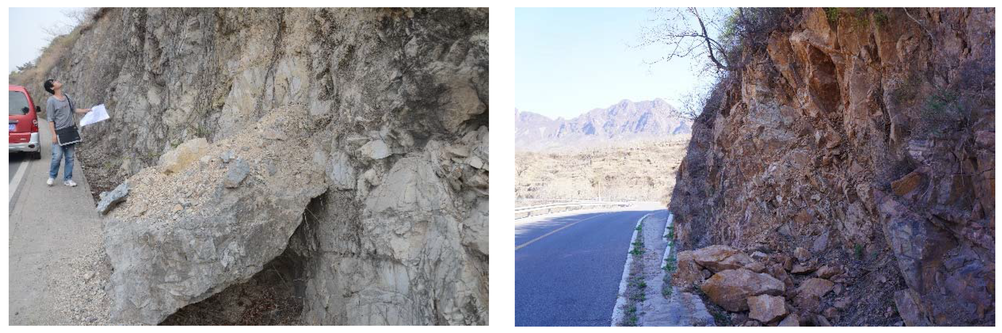
Figure 3.
Thematic layers of the classified conditional factors: (a) lithology; (b) slope angle; (c) slope aspect; (d) slope curvature; (e) topographic elevation; (f) distance to faults; (g) NDVI; and (h) distance to roads.
Figure 3.
Thematic layers of the classified conditional factors: (a) lithology; (b) slope angle; (c) slope aspect; (d) slope curvature; (e) topographic elevation; (f) distance to faults; (g) NDVI; and (h) distance to roads.
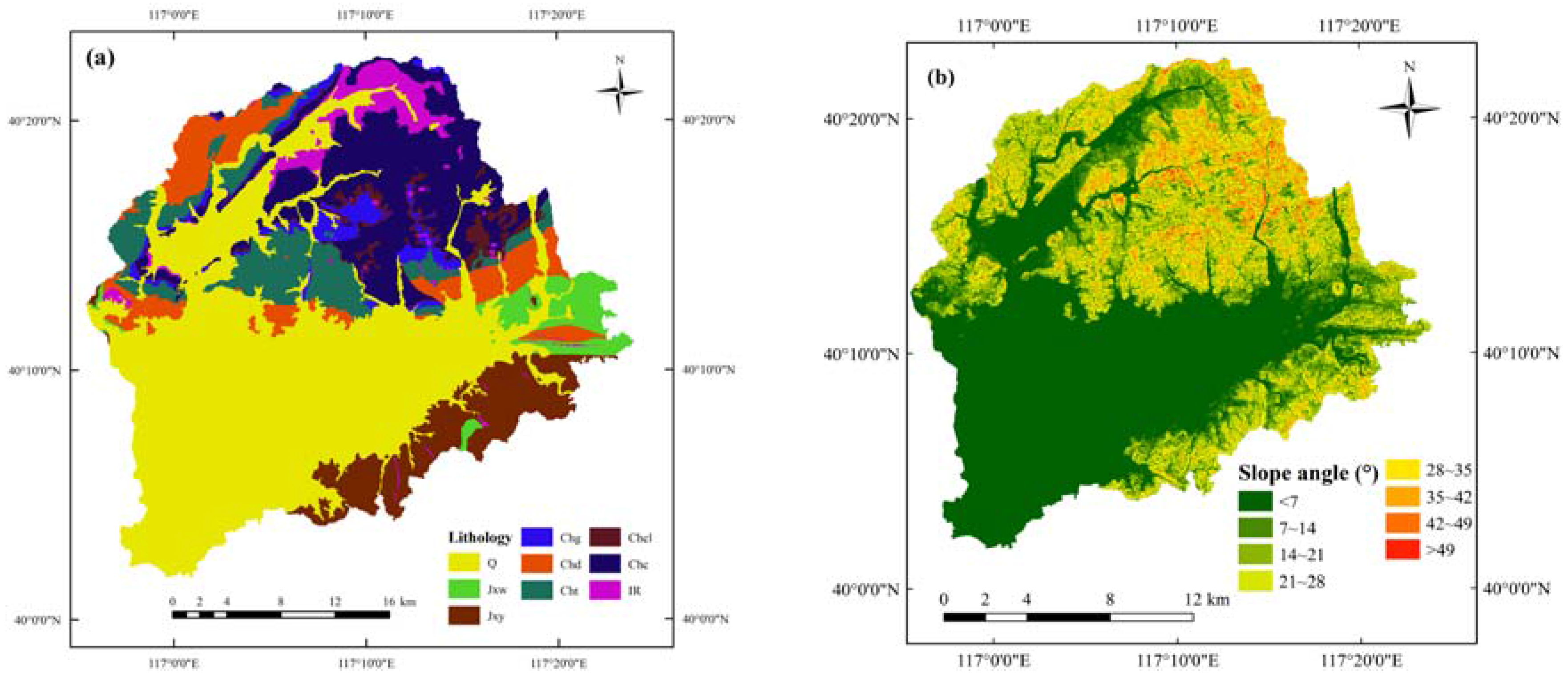
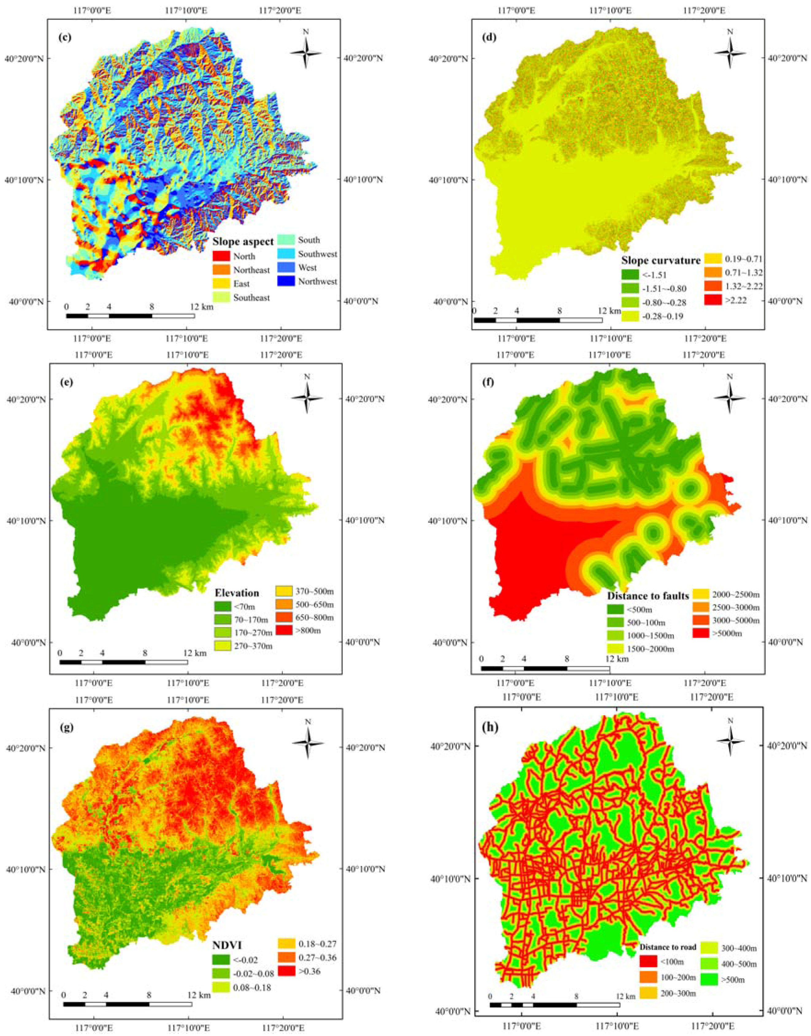
Figure 4.
Variations of the computed FRs and CFs for each class/type of the conditional factors.

Figure 5.
Landslide susceptibility maps using (a) the frequency ratio, and (b) the certainty factor.
Figure 5.
Landslide susceptibility maps using (a) the frequency ratio, and (b) the certainty factor.

Figure 6.
The area under curve analysis: (a) success rate curve using the training dataset; and (b) predicted curve using the validating dataset.
Figure 6.
The area under curve analysis: (a) success rate curve using the training dataset; and (b) predicted curve using the validating dataset.

Table 1.
Description of geological units in the study area.
| Geological age | Formation | Lithology | Class |
|---|---|---|---|
| Cenozoic | -- | Quaternary deposits, gravelly soils. | Q |
| Proterozoic | Wumishan | Dolomite, silty dolomite, silty dolomite, argillaceous dolomite, shale. | Jxw |
| Yangzhuang | Conglomeratic dolomite, argillaceous and silty dolomicrite, carneule. | Jxy | |
| Gaoyuzhuang | Sandy dolomite, silty dolomite. | Chg | |
| Dahongyu | Dolomitic quartz sandstone, dolomicrite. | Chd | |
| Tuanzishan | Silty dolomicrite, dolomite, dolomicrite with siltstone and shale. | Cht | |
| Cuanlinggou | Lamellar sandy shale, dolomitic siltstone, dolomitic sandstone with silty shale. | Chcl | |
| Changzhougou | Silty shale, feldspathic quartz sandstone with siltstone, lenticular hematite. | Chc | |
| Archaeozoic | -- | Igneous rocks such as quartz monzonite, sillite, granite. | IR |
Table 2.
Weighted values calculated for each category of the conditional factors, based on the FR model and the CF model.
Table 2.
Weighted values calculated for each category of the conditional factors, based on the FR model and the CF model.
| Factor | Class | Npix(Ni,j) | Npix(Si,j) | PPa | PPs | FRi,j | CF |
|---|---|---|---|---|---|---|---|
| Lithology | Q | 512,803 | 413 | 0.0008 | 0.0017 | 0.4838 | −0.5166 |
| Jxw | 87,244 | 116 | 0.0013 | 0.0017 | 0.7988 | −0.2015 | |
| Jxy | 38,041 | 194 | 0.0051 | 0.0017 | 3.0638 | 0.6747 | |
| Chg | 80,374 | 60 | 0.0007 | 0.0017 | 0.4485 | −0.5519 | |
| Chd | 88,020 | 120 | 0.0014 | 0.0017 | 0.8190 | −0.1812 | |
| Cht | 31,522 | 52 | 0.0016 | 0.0017 | 0.9911 | −0.0090 | |
| Chcl | 23,553 | 21 | 0.0009 | 0.0017 | 0.5357 | −0.4648 | |
| Chc | 154,381 | 636 | 0.0041 | 0.0017 | 2.4750 | 0.5969 | |
| IR | 39,014 | 144 | 0.0037 | 0.0017 | 2.2174 | 0.5499 | |
| Slope | <7° | 506,984 | 158 | 0.0003 | 0.0017 | 0.1872 | −0.8130 |
| 7°~14° | 118,489 | 269 | 0.0023 | 0.0017 | 1.3639 | 0.2673 | |
| 14°~21° | 136,524 | 354 | 0.0026 | 0.0017 | 1.5578 | 0.3587 | |
| 21°~28° | 128,646 | 403 | 0.0031 | 0.0017 | 1.8820 | 0.4694 | |
| 28°~35° | 100,066 | 321 | 0.0032 | 0.0017 | 1.9272 | 0.4819 | |
| 35°~42° | 50,783 | 196 | 0.0039 | 0.0017 | 2.3187 | 0.5697 | |
| 42°~49° | 11,954 | 51 | 0.0043 | 0.0017 | 2.5631 | 0.6109 | |
| >49° | 1506 | 4 | 0.0027 | 0.0017 | 1.5957 | 0.3739 | |
| Aspect | N | 103,652 | 129 | 0.0012 | 0.0017 | 0.7477 | −0.2526 |
| NE | 91,548 | 160 | 0.0017 | 0.0017 | 1.0500 | 0.0477 | |
| E | 111,586 | 120 | 0.0011 | 0.0017 | 0.6461 | −0.3543 | |
| SE | 130,747 | 126 | 0.0010 | 0.0017 | 0.5790 | −0.4214 | |
| S | 167,337 | 308 | 0.0018 | 0.0017 | 1.1058 | 0.0958 | |
| SW | 164,646 | 445 | 0.0027 | 0.0017 | 1.6237 | 0.3848 | |
| W | 166,578 | 305 | 0.0018 | 0.0017 | 1.1000 | 0.0911 | |
| NW | 118,858 | 163 | 0.0014 | 0.0017 | 0.8239 | −0.1764 | |
| Curvature | >–1.51 | 22,004 | 38 | 0.0017 | 0.0017 | 1.0375 | 0.0362 |
| −1.51~−0.80 | 75,504 | 172 | 0.0023 | 0.0017 | 1.3686 | 0.2698 | |
| −0.80~−0.28 | 127,940 | 408 | 0.0032 | 0.0017 | 1.9159 | 0.4788 | |
| −0.28~0.19 | 600,592 | 553 | 0.0009 | 0.0017 | 0.5532 | −0.4472 | |
| 0.19~0.71 | 111,692 | 333 | 0.0030 | 0.0017 | 1.7911 | 0.4424 | |
| 0.71~1.32 | 73,454 | 186 | 0.0025 | 0.0017 | 1.5213 | 0.3432 | |
| 1.32~2.22 | 35,762 | 65 | 0.0018 | 0.0017 | 1.0919 | 0.0843 | |
| >2.22 | 8004 | 1 | 0.0001 | 0.0017 | 0.0751 | −0.9251 | |
| Elevation | <70 m | 383,802 | 67 | 0.0002 | 0.0017 | 0.1049 | −0.8953 |
| 70~170 m | 190,001 | 435 | 0.0023 | 0.0017 | 1.3754 | 0.2734 | |
| 170~270 m | 157,372 | 496 | 0.0032 | 0.0017 | 1.8935 | 0.4727 | |
| 270~370 m | 117,464 | 343 | 0.0029 | 0.0017 | 1.7543 | 0.4307 | |
| 370~500 m | 87,612 | 227 | 0.0026 | 0.0017 | 1.5566 | 0.3582 | |
| 500~650 m | 62,203 | 96 | 0.0015 | 0.0017 | 0.9272 | −0.0729 | |
| 650~800 m | 35,080 | 81 | 0.0023 | 0.0017 | 1.3872 | 0.2796 | |
| >800 m | 21,418 | 11 | 0.0005 | 0.0017 | 0.3085 | −0.6918 | |
| Distance to fault | <500 m | 186,708 | 496 | 0.0027 | 0.0017 | 1.5960 | 0.3740 |
| 500~1000 m | 157,821 | 296 | 0.0019 | 0.0017 | 1.1268 | 0.1127 | |
| 1000~1500 m | 133,401 | 225 | 0.0017 | 0.0017 | 1.0133 | 0.0131 | |
| 1500~2000 m | 104,352 | 268 | 0.0026 | 0.0017 | 1.5429 | 0.3525 | |
| 2000~2500 m | 79,364 | 290 | 0.0037 | 0.0017 | 2.1952 | 0.5454 | |
| 2500~3000 m | 57,988 | 40 | 0.0007 | 0.0017 | 0.4144 | −0.5860 | |
| 3000~5000 m | 133,762 | 117 | 0.0009 | 0.0017 | 0.5255 | −0.4749 | |
| >5000 m | 201,556 | 24 | 0.0001 | 0.0017 | 0.0715 | −0.9286 | |
| NDVI | <−0.02 | 174,033 | 38 | 0.0002 | 0.0017 | 0.1312 | –0.8690 |
| −0.02~0.08 | 133,598 | 160 | 0.0012 | 0.0017 | 0.7195 | −0.2808 | |
| 0.08~0.18 | 141,626 | 280 | 0.0020 | 0.0017 | 1.1877 | 0.1583 | |
| 0.18~0.27 | 226,641 | 534 | 0.0024 | 0.0017 | 1.4155 | 0.2940 | |
| 0.27~0.36 | 239,948 | 458 | 0.0019 | 0.0017 | 1.1467 | 0.1282 | |
| >0.36 | 139,106 | 286 | 0.0021 | 0.0017 | 1.2352 | 0.1907 | |
| Distance to road | <100 m | 291,382 | 833 | 0.0029 | 0.0017 | 1.7175 | 0.4145 |
| 100~200 m | 191,086 | 613 | 0.0032 | 0.0017 | 1.9273 | 0.4695 | |
| 200~300 m | 160,410 | 211 | 0.0013 | 0.0017 | 0.7902 | −0.2356 | |
| 300~400 m | 102,657 | 75 | 0.0007 | 0.0017 | 0.4389 | −0.5886 | |
| 400~500 m | 84,483 | 24 | 0.0002 | 0.0017 | 0.1707 | −0.8825 | |
| >500 m | 224,934 | 0 | 0 | 0.0017 | 0 | −1 |
© 2017 by the authors. Licensee MDPI, Basel, Switzerland. This article is an open access article distributed under the terms and conditions of the Creative Commons Attribution (CC BY) license (http://creativecommons.org/licenses/by/4.0/).
Share and Cite
MDPI and ACS Style
Deng, X.; Li, L.; Tan, Y. Validation of Spatial Prediction Models for Landslide Susceptibility Mapping by Considering Structural Similarity. ISPRS Int. J. Geo-Inf. 2017, 6, 103. https://doi.org/10.3390/ijgi6040103
AMA Style
Deng X, Li L, Tan Y. Validation of Spatial Prediction Models for Landslide Susceptibility Mapping by Considering Structural Similarity. ISPRS International Journal of Geo-Information. 2017; 6(4):103. https://doi.org/10.3390/ijgi6040103
Chicago/Turabian StyleDeng, Xiaolong, Lihui Li, and Yufang Tan. 2017. "Validation of Spatial Prediction Models for Landslide Susceptibility Mapping by Considering Structural Similarity" ISPRS International Journal of Geo-Information 6, no. 4: 103. https://doi.org/10.3390/ijgi6040103
Note that from the first issue of 2016, this journal uses article numbers instead of page numbers. See further details here.