Attribute Learning for SAR Image Classification


Electronic and Information School, Wuhan University, Wuhan 430072, China
*
Author to whom correspondence should be addressed.
ISPRS Int. J. Geo-Inf. 2017, 6(4), 111; https://doi.org/10.3390/ijgi6040111
Submission received: 17 January 2017
/
Revised: 29 March 2017
/
Accepted: 1 April 2017
/
Published: 5 April 2017
Abstract
:This paper presents a classification approach based on attribute learning for high spatial resolution Synthetic Aperture Radar (SAR) images. To explore the representative and discriminative attributes of SAR images, first, an iterative unsupervised algorithm is designed to cluster in the low-level feature space, where the maximum edge response and the ratio of mean-to-variance are included; a cross-validation step is applied to prevent overfitting. Second, the most discriminative clustering centers are sorted out to construct an attribute dictionary. By resorting to the attribute dictionary, a representation vector describing certain categories in the SAR image can be generated, which in turn is used to perform the classifying task. The experiments conducted on TerraSAR-X images indicate that those learned attributes have strong visual semantics, which are characterized by bright and dark spots, stripes, or their combinations. The classification method based on these learned attributes achieves better results.
1. Introduction
Synthetic Aperture Radar (SAR) is characterized by day-and-night and all-weather imaging ability in remote sensing; moreover, SAR images contain rich information on the imaged area, i.e., the dielectric and geometrical characteristics of the observed object are relevant to the backscattering [1]. Therefore, SAR plays an increasingly important role in various applications, such as urban planning, environmental monitoring, geoscience research, etc. In recent years, with improvements of SAR systems in terms of spatial resolution, high resolution SAR images can provide more detailed and precise information on an observed scene; for this reason, the application of SAR data is highly popular in earth observation [2]. Meanwhile, it also creates challenges in SAR image classification because of the more sophisticated shapes, structures and other details of the target. Consequently, it would be highly desirable to interpret SAR images based on a multi-layer model with clear semantic attributes.
Over the last two decades, several methods have been proposed for SAR image interpretation. Roughly speaking, these methods can be categorized into, but not limited to, statistical-based, texture-based and model-based methods. Statistical-based methods mainly relied on the fact that SAR images are characterized by statistical properties. Various statistical models have been proposed, e.g., Lognormal, Rayleigh, Fisher distribution [3], [4], etc. Texture-based approaches include the Gray-Level Co-occurrence Matrix (GLCM) [5], Gabor filter [6], sparse coding of wavelet polarization textons [7], etc. Model-based methods, e.g., Markov Random Fields (MRFs) [8], Conditional Random Fields [9], Bayesian Network (BN) [10], are widely used for image analysis. In addition, with improvements in spatial resolution, several works have considered spatial features, e.g., morphological profiles, attribute profiles [11,12,13]. Recently, the Bag-of-Word (BoW) model has been introduced for SAR image classification [14,15], which is inspired by the texton representation of an image, and this approach is based on the discriminative low-level features. The multi-layer model is a useful framework for SAR image classification tasks in the case of complex scenes [16]. However, high-level features extracted by the multi-layer model often lack semantics, and it is an intractable problem to directly establish a correspondence between the physical mechanisms of a SAR image and the semantics of the features at a high level.
Recently, attribute learning has received increasing attention in the computer vision community [17,18], and its effectiveness has been demonstrated in various applications. For example, image retrieval based on weak attributes was proposed in [19], color attributes were applied to object detection [20]; in [21], between-class attributes were utilized to object classification when training and test classes are disjoint. However, the attribute of the SAR image, by contrast, is quite different from the one in optical image because of the coherent imagery mechanism in SAR. Consequently, there are two problems waiting to be solved in the interpretation of the SAR image. The first issue is how to explore the elemental attribute for coherent imagery. On the other hand, the features extracted by the multi-layer model often lack semantic attributes, namely the semantic gap that exists between the extracted features and interpretation; therefore, explainable feature learning by the multi-layer model is another problem for understanding SAR images.
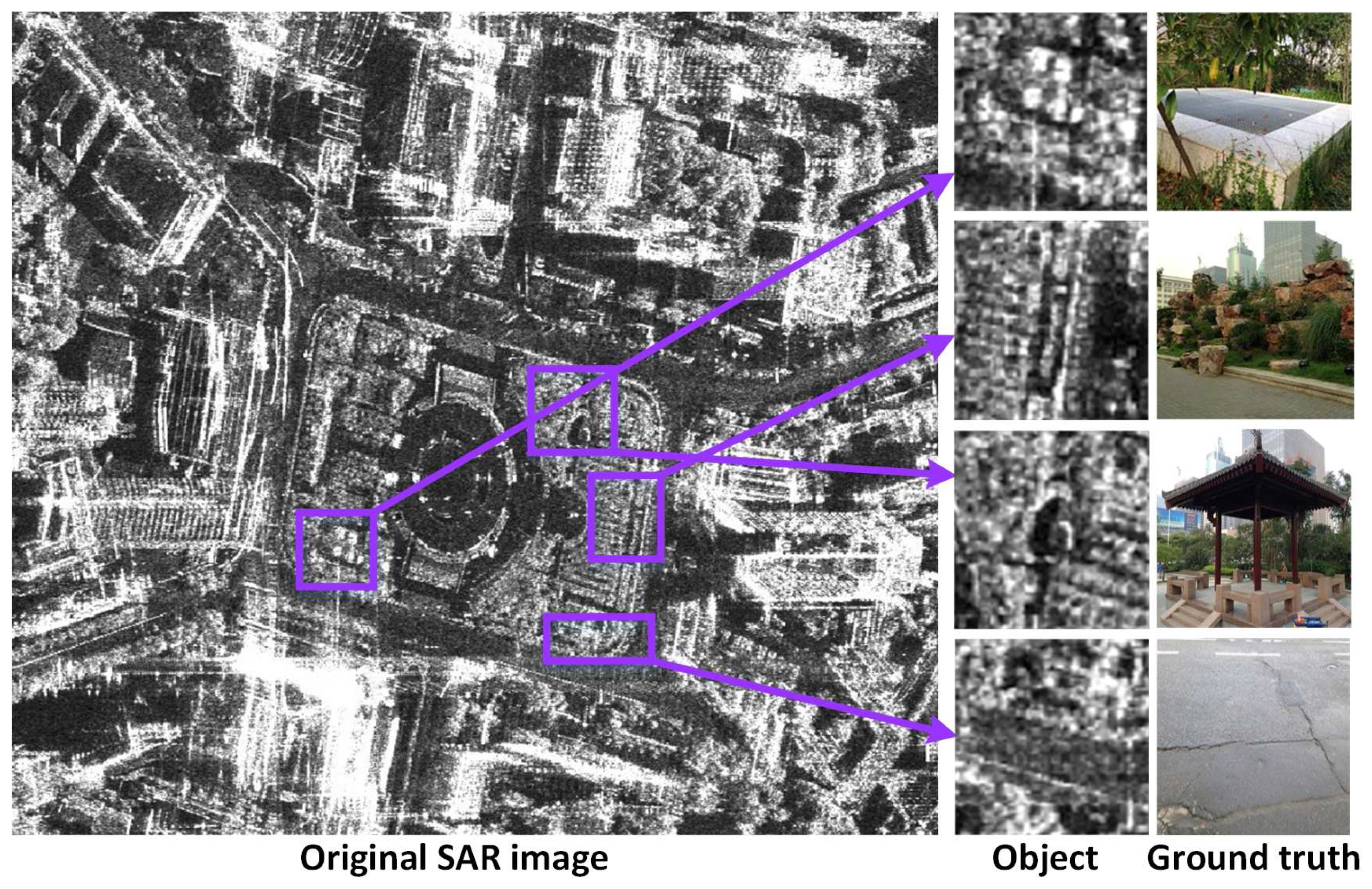
With the spatial resolution improvement in high-resolution SAR, the objects of interest are no longer limited within several pixels, and more complex and rich information is provided, such as the structures, shapes and other details. As shown in Figure 1, different objects in this SAR image, which was acquired by TerraSAR-X, exhibit evidently visual semantics, i.e., bright and dark single spots, dense spots, a linear stripe, or their combination. In this paper, the attributes of the SAR image are referred to as these visual semantics.
In this paper, a classification method based attribute learning for SAR images is presented. The main contribution is that we explore the learning attributes of SAR images. In order to learn the discriminative attributes, an unsupervised clustering algorithm [22] is applied to find clustering centers in the space of low-level features, including the ratio of mean-to-variance and the maximum ratio of means in four different directions of an patch, which is sampled at multiple scales from the input image; then, the most discriminative clusters are sorted out to form an attribute dictionary. During the procedure for learning those attributes, cross-validation is applied at each step to prevent overfitting, and the most discriminative clusters are ranked based on the scores from Support Vector Machine (SVM) [23]. Specifically, these learned attributes possess semantic properties, which is demonstrated by the experimental results, and the classification method shows promising performance.
2. Attribute Learning
The input image is first partitioned into several patches with multiscale; then, low-level features, including maximum edge response and the ratio of mean-to-variance, are extracted for each patch; the last step is iterative clustering in the feature space, and the discriminative and representative features are sorted out to construct an attribute dictionary.
2.1. Low-Level Feature Extraction
Because of the presence of speckle noise in SAR imaging, such low-level features, which are robust to the impact of speckles, are desirable in SAR image representation. Here, ratio-based features, namely, the maximum edge response and the ratio of mean-to-variance, are selected for low-level image representation.
The edge response [24] is defined as the ratio of mean values in two non-overlap neighborhoods of a patch; to detect all potential edges, the edge response should be computed in all directions in the patch. Here, four elemental directions are considered, which are shown in Figure 2, i.e., and , and the maximum edge response is used to describe the edge of the local patch. The maximum edge response is defined as
where denotes the edge response in ith direction, and is given by [25]
where and are the average of pixel values in two neighborhoods.
For the ratio of mean-to-variance , which is a statistical feature for a patch, it is defined by
where u and denote the mean and variance of the sampled patch.
Both and are used to represent a patch, and therefore, the extracted feature vector with two elements, is given by
where represents the transpose operation.
2.2. Attribute Learning
The goal of this paper is to exploit a set of representative and discriminative mid-level features, which are expected to describe the attributes of an SAR image. In other words, the correspondence between these features and the attributes should be bridged. To explore and discover the underlying relationships between them, unsupervised clustering algorithms are needed for this task.
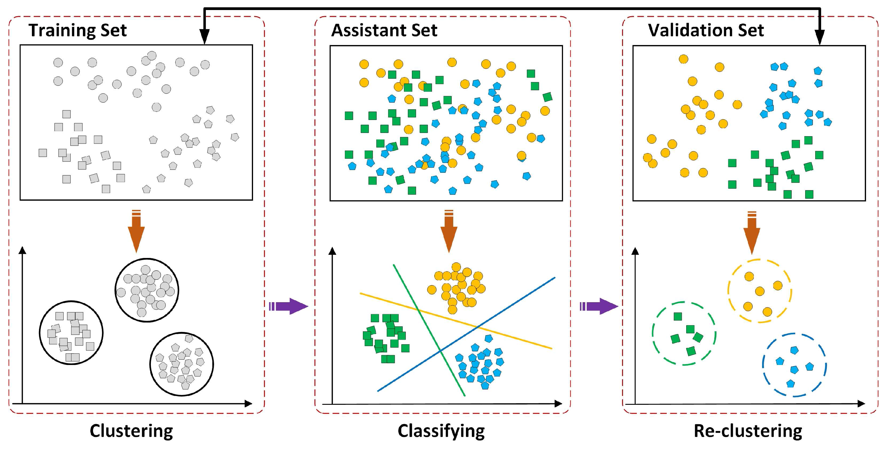
A large number of clustering methods, e.g., k-means [26], can be used to deal with a standard unsupervised clustering problem. However, as noted in [22], because of the low-level distance metric adopted by these clustering methods, e.g., L1, Euclidean, Cross-correlation, these methods often result in poor performance in clustering tasks with mid-level features. With the discriminative requirement of the desirable attributes, in this paper, an iterative learning step, as illustrated in Figure 3, is employed for this requirement. This procedure is implemented in Algorithm 1, and each step is summarized as follows.
| Algorithm 1 Attribute learning |
| Input: Training set , validation set , assistant set |
| Output: Attributes |
| Step |
| 1: While: not convergence do |
| 2: Exchange: and |
| 3: Cluster on , cluster center , |
| remove cluster centers with less than 3 members |
| 4: Train corresponding classifiers on with positive examples from step 3 |
| 5: Classify on , top 5 members are sorted out for each new cluster |
| 6: Swap |
| 7: Repeat step 3 to 5 |
| 8: if members are not changed in each cluster center |
| 9: end while |
| 10: return Attributes |
The input full scene is divided into two equal but non-overlaping subsets, i.e., the training subset and validation subset . Another required dataset , called the assistant set, is formed by collecting images from the same SAR system. For all images in the training set , first, n patches are sampled at multiple scales. For each image, the patch size ranges from the local region, e.g., pixel, to global size, and an overlap sampling strategy, namely, stride pixels, is applied to cover the entire image [15]. Then, low-level features are extracted for each patch, including the maximum edge response and the ratio of mean-to-variance; next, standard k-means is employed to cluster in the low-level feature space, where the clustering center is and where n is the number of patches in dataset . Considering the representative requirement, cluster centers with less than three members are removed, and m clusters remain.
The next step is to train a linear SVM classifier for each cluster generated in the first step, where the positive examples are the members within each cluster, whereas the negative examples come from the assistant dataset . Then, the trained classifiers are applied to perform classification on the cross-validation subset , and those labeled samples are re-clustered to form new cluster centers. Note that the members of each cluster center only come from the top samples with higher classified scores. Parameters for attribute learning are summarized in Table 1.
When the new clusters are constructed, the training set and validation set are exchanged; then, the above clustering and classification steps are iteratively repeated, and those clusters that were fired less than 2 times are removed. The procedure described above is iterated until convergence, i.e., the members within each cluster do not change. Note that some low-level features are removed during this procedure since they are not representative and discriminative.
2.3. Attribute Dictionary Construction
The attribute dictionary consists of the most distinctive attributes, namely, the cluster centers with maximum separation. To construct such an attribute dictionary an SVM classifier is first employed on the clustering centers, which have been generated during the attribute learning step, and new clusters are generated; Then, the classified scores are assigned to these new clusters, where the classified scores are computed by summing up the scores of the top r (where ) members within the new cluster based on the confidence of SVM classification. Finally, the top K clusters are selected to construct the attribute dictionary , where is the kth selected cluster center. Once we have built this attribute dictionary, the ith patch, sampled from the input image and represented by feature , can be represented by a dictionary-based feature vector ; the kth element is given by
For all patches from an input SAR image, such a feature vector can be obtained by Equation (5). As a consequence, the input SAR image can be described by a statistical histogram , and is the sum-pooling of , where n is the number of sampled patches, and the kth element in is the sum of the kthe elements in .
3. Classification with Attributes
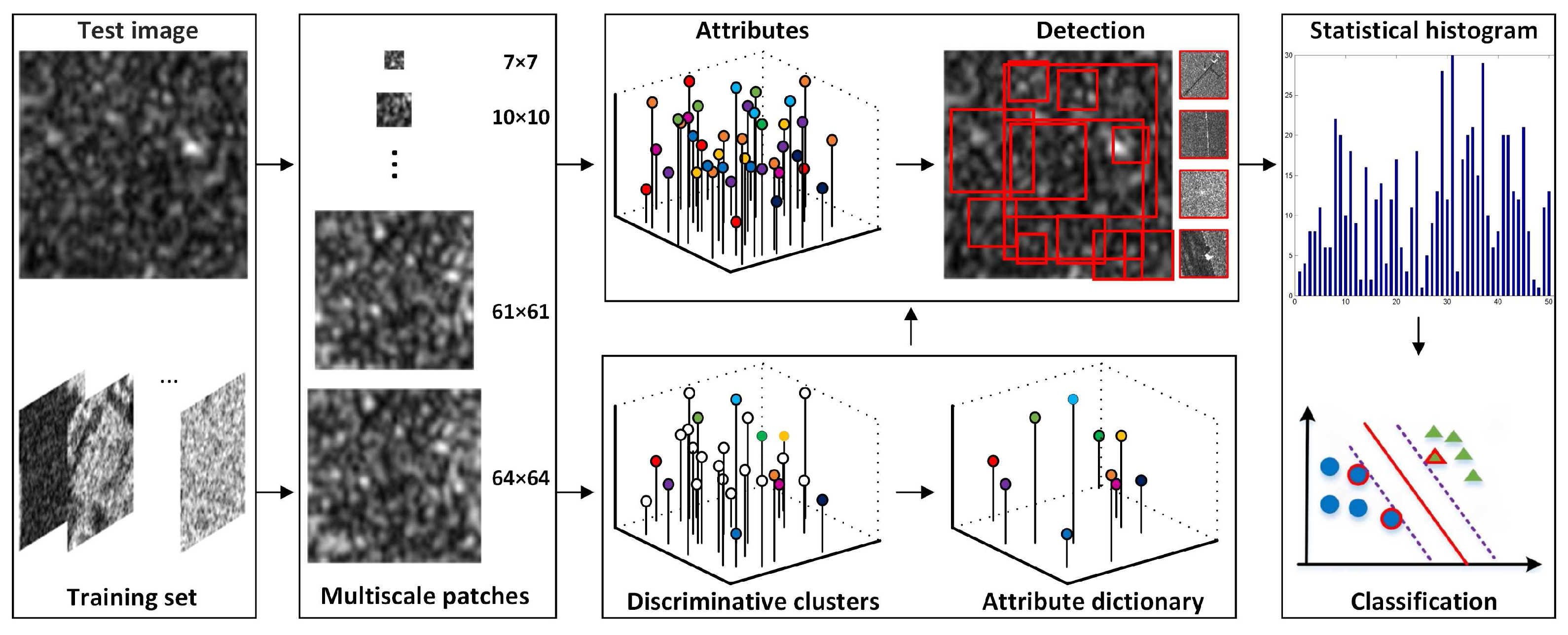
As illustrated in Figure 4, the classifying framework is composed of three steps, namely: the low-level feature extraction, attribute detection, and classification steps.
The first step is low-level feature extraction for the input SAR image; several patches are first sampled at multiple scales from the input image; then, the low-level features can be extracted by computing the maximum edge response and the ratio of mean-to-variance; these extracted features are the candidates to be detected for the representation of the input image.
The second step is attribute detection. The attributes for the test image can be sorted out by referring to the attribute dictionary, where the metric is based on the nearest neighbor. Note that these detected attributes correspond to the multi-scale patches sampled from the test image. This is equivalent to detecting visual words for the image.
The last step is the implementation of classification. When the attributes have been sorted out, a statistical histogram describing the attributes frequency can be computed as a final descriptor; then, a simple linear SVM is applied to perform classification.
4. Experiment
4.1. Data Set
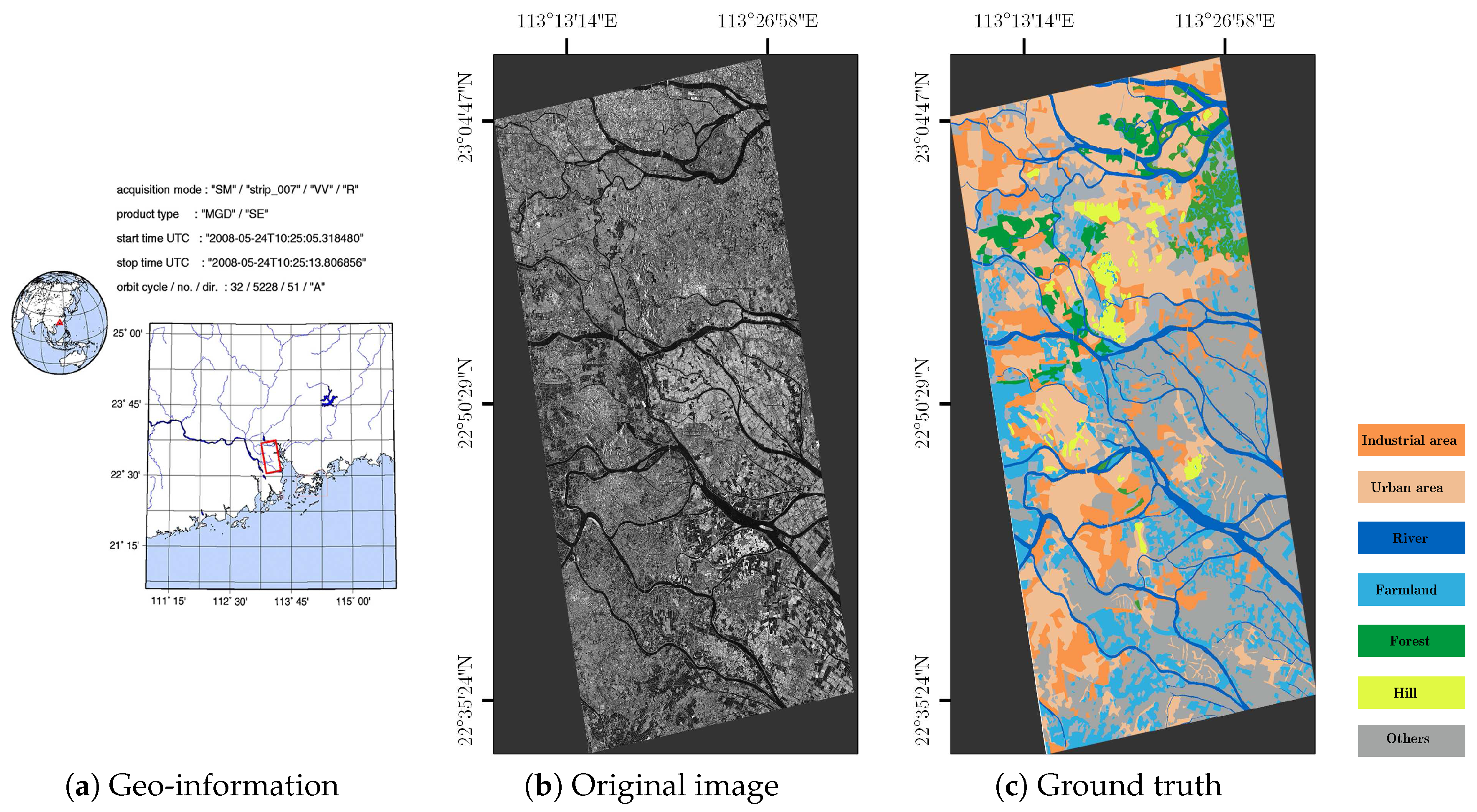
To evaluate the performance of the proposed method, a data set is collected. This full scene was acquired by TerraSAR-X with single polarization (VV channel) from an area in Guangdong Province, China on 24 May 2008. The full scene is composed of 7 categories as shown in Figure 5, including forest, river, hill, farmland, industrial area, urban region and others. Each category contains 160 images with a size of pixels and a pixel spacing of about 1.25 meters. The dataset and for model training are formed by sampling 100 images in each category, and the remaining images are used to test. The assistant dataset is formed by a collection of images from the same TerraSAR-X system.
4.2. Parameter Setting
There are 350 images in each dataset and , and 2000 images in the assistant dataset . The minimum patch size used to extract low-level features is pixels with a stride of 7 pixels, and the maximum size is as large as the entire image size; those patches are generated by sampling the input image at 19 multiple scales. During the step of initial clustering, the cluster center is , where n is the number of patches in dataset ; the member of cluster thought to be fired is based on the SVM score, which is set above −1. The total number of the attributes sorted out to form the attribute dictionary, is 3396, and the top 1000 discriminative attributes are used for image representation.
4.3. Results and Analysis
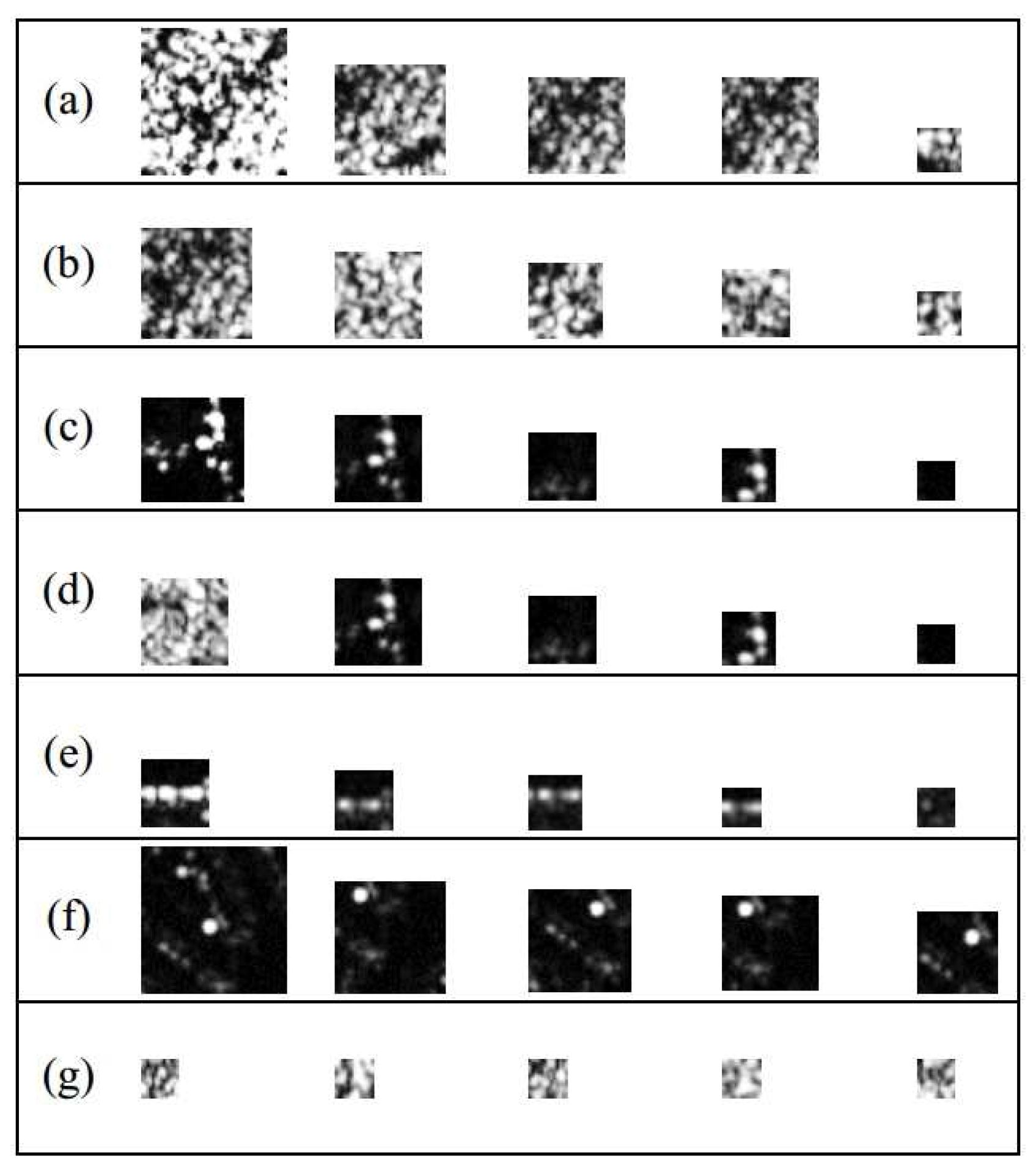
The most discriminative 5 patches for each category are shown in Figure 6. Here, the detected patches from (a) to (g) correspond to the categories in Figure 5.
As noted, the discriminative patches among categories are quite different; e.g., the patches in (b) are characterized by dense spots, the patches in (e) by stripe, and the patches in (f) are a combination of a single spot and stripe. Moreover, there is remarkable resemblance among the discriminative patches within each category, e.g., the characterization of dense spots in (a) and linear bright stripe in (e). This demonstrates that the learned attributes are representative and discriminative since the interactive algorithm, including initial clustering, classifying and re-clustering step, is used during the attribute learning. The clustering step will sort out the frequently occurring cluster centers, namely, the representative attributes, while the classification step will ensure that these selected attributes are quite discriminative from the rest.
To evaluate the performance of the proposed method, five state-of-the-art methods are chosen for comparison, including GLCM [5], Gabor [6], GMRF [27], Particle Filter Sample Texton (PFST) [28] and BoW-MV [25]; the settings for each method are described as follows. There are 4 extracted statistical features for GLCM, i.e., contrast, correlation, energy and inverse different moment. Gabor filters are implemented on 8 orientations and 3 linear scales, and the mean and variance of each sub band form the Gabor texture feature. The GMRF texture features are generated by estimating the 4-level GMRG model with 12 parameters. For the PFST, the patch size is pixels; there are 8 key points and 10 texton per class. The cell for local feature extraction in BoW-MV is pixels.
Table 2 shows the classification results; here, AL, the abbreviation of Attribute Learning, denotes the proposed method. Besides the classification accuracy for each class and average accuracy (A.A.), the Kappa coefficients (Kappa) and Kappa confidence intervals (Kappa C.I.) [29] are also used for comparison. The average accuracy of the proposed method is slightly better than other approaches; for example, compared with the state-of-the-art method PFST, the Kappa confidence interval, 0.83 to 0.89, is more confident, and the average accuracy and Kappa coefficients are improved by 7.5% and 0.06%, respectively. Moreover, the classification accuracy of the proposed approach is obviously improved on a region with such rich structure information, such as the industrial and hill area; this is because the edge detector and the ratio of mean-to-variance are extracted as low-level features.
5. Conclusions
This paper has presented a classification method based on attribute learning for high spatial resolution SAR images. The key contribution is that attributes for SAR images have been extracted, which are characterized by bright and dark spots, stripes, or various combinations of them. In order to learn these attributes, an iterative procedure was designed, including unsupervised clustering step, classification training step, and a cross-validation for preventing over-fitting. The experiments conducted on TerraSAR-X data demonstrate that the extracted attributes are discriminative and representative, and the classification method, based on the learned attributes, achieved better accuracy, especially on regions with rich structure information. However, the proposed method is not rotation-invariant; further research is required to address this issue for performance improvement.
Acknowledgments
This work was partially supported by the National Natural Science Foundation of China under grant No.61331016, No.41371342, and by the National Key Basic Research and Development Program of China (973 Program) under grant No.2013CB733404.
Author Contributions
Chu He and Xinlong Liu conceived and designed the experiments; Chenyao Kang performed the experiments and analyzed the results; Chu He and Xinlong Liu wrote the paper; Dong Chen, Mingsheng Liao revised the paper.
Conflicts of Interest
The authors declare no conflict of interest.
References
- Moreira, A.; Prats-Iraola, P.; Younis, M.; Krieger, G.; Hajnsek, I.; Papathanassiou, K.P. A tutorial on synthetic aperture radar. IEEE Geosci. Remote Sens. Mag. 2013, 1, 6–43. [Google Scholar] [CrossRef]
- Reigber, A.; Scheiber, R.; Jager, M.; Prats-Iraola, P.; Hajnsek, I.; Jagdhuber, T.; Papathanassiou, K.P.; Nannini, M.; Aguilera, E.; Baumgartner, S.; et al. Very-high-resolution airborne synthetic aperture radar imaging: Signal processing and applications. Proc. IEEE 2013, 101, 759–783. [Google Scholar] [CrossRef]
- Tison, C.; Nicolas, J.M.; Tupin, F.; Maître, H. A new statistical model for Markovian classification of urban areas in high-resolution SAR images. IEEE Trans. Geosci. Remote Sens. 2004, 42, 2046–2057. [Google Scholar] [CrossRef]
- Marques, R.C.P.; Medeiros, F.N.; Nobre, J.S. SAR image segmentation based on level set approach and model. IEEE Trans. Pattern Anal. Mach. Intell. 2012, 34, 2046–2057. [Google Scholar] [CrossRef] [PubMed]
- Haralick, R.M.; Shanmugam, K.; Dinstein, I. Textural features for image classification. IEEE Trans. Syst. Man Cybern. 1973, SMC-3, 610–621. [Google Scholar] [CrossRef]
- Torres-Torriti, M.; Jouan, A. Gabor vs. GMRF features for SAR imagery classification. In Proceedings of the 2001 International Conference on Image Processing (ICIP), Thessaloniki, Greece, 7–10 October 2001; pp. 1043–1046. [Google Scholar]
- He, C.; Li, S.; Liao, Z.; Liao, M. Texture classification of PolSAR data based on sparse coding of wavelet polarization textons. IEEE Trans. Geosci. Remote Sens. 2013, 51, 4576–4590. [Google Scholar] [CrossRef]
- Li, S.Z. Markov Random Field Modeling in Image Analysis; Springer Science & Business Media: New York, NY, USA, 2009. [Google Scholar]
- Lafferty, J.D.; Mccallum, A.; Pereira, F.C.N. Conditional random fields: Probabilistic models for segmenting and labeling sequence data. In Proceedings of the Eighteenth International Conference on Machine Learning, Williams College, MA, USA, 28 June–1 July 2001; pp. 282–289. [Google Scholar]
- Koller, D.; Friedman, N. Probabilistic Graphical Models: Principles and Techniques; MIT Press: Cambridge, MA, USA, 2009. [Google Scholar]
- Ghamisi, P.; Souza, R.; Benediktsson, J.A.; Zhu, X.X.; Rittner, L.; Lotufo, R.A. Extinction profiles for the classification of remote sensing data. IEEE Trans. Geosci. Remote Sens. 2016, 54, 5631–5645. [Google Scholar] [CrossRef]
- Geiß, C.; Klotz, M.; Schmitt, A.; Taubenböck, H. Object-based morphological profiles for classification of remote sensing imagery. IEEE Trans. Geosci. Remote Sens. 2016, 54, 5952–5963. [Google Scholar] [CrossRef]
- Demir, B.; Bruzzone, L. Histogram-based attribute profiles for classification of very high resolution remote sensing images. IEEE Trans. Geosci. Remote Sens. 2016, 54, 2096–2107. [Google Scholar] [CrossRef]
- Feng, J.; Jiao, L.; Zhang, X.; Yang, D. Bag-of-visual-words based on clonal selection algorithm for SAR image classification. IEEE Geosci. Remote Sens. Lett. 2011, 8, 691–695. [Google Scholar] [CrossRef]
- Cui, S.; Schwarz, G.; Datcu, M. Remote sensing image classification: No features, no clustering. IEEE J. Sel. Top. Appl. Earth Obs. Remote Sens. 2015, 8, 5158–5170. [Google Scholar] [CrossRef]
- He, C.; Zhuo, T.; Ou, D.; Liu, M.; Liao, M. Nonlinear compressed sensing-based LDA topic model for polarimetric SAR image classification. IEEE J. Sel. Top. Appl. Earth Obs. Remote Sens. 2014, 7, 972–982. [Google Scholar] [CrossRef]
- Parikh, D.; Grauman, K. Relative attributes. In Proceedings of the 2011 IEEE International Conference on Computer Vision (ICCV), Barcelona, Spain, 6–13 November 2011; pp. 503–510. [Google Scholar]
- Scheirer, W.J.; Kumar, N.; Belhumeur, P.N.; Boult, T.E. Multi-attribute spaces: Calibration for attribute fusion and similarity search. In Proceedings of the 2012 IEEE Conference on Computer Vision and Pattern Recognition (CVPR), Providence, RI, USA, 16–21 June 2012; pp. 2933–2940. [Google Scholar]
- Felix, X.Y.; Ji, R.; Tsai, M.H.; Ye, G.; Chang, S.F. Weak attributes for large-scale image retrieval. In Proceedings of the 2012 IEEE Conference on Computer Vision and Pattern Recognition (CVPR), Providence, RI, USA, 16–21 June 2012; pp. 2949–2956. [Google Scholar]
- Khan, F.S.; Anwer, R.M.; Van De Weijer, J.; Bagdanov, A.D.; Vanrell, M.; Lopez, A.M. Color attributes for object detection. In Proceedings of the 2012 IEEE Conference on Computer Vision and Pattern Recognition (CVPR), Providence, RI, USA, 16–21 June 2012; pp. 3306–3313. [Google Scholar]
- Lampert, C.H.; Nickisch, H.; Harmeling, S. Learning to detect unseen object classes by between-class attribute transfer. In Proceedings of the 2009 IEEE Conference on Computer Vision and Pattern Recognition, Miami, FL, USA, 20–25 June 2009; pp. 951–958. [Google Scholar]
- Singh, S.; Gupta, A.; Efros, A.A. Unsupervised discovery of mid-level discriminative patches. In Computer Vision–ECCV 2012; Springer: New York, NY, USA, 2012; pp. 73–86. [Google Scholar]
- Fukuda, S.; Hirosawa, H. Support vector machine classification of land cover: Application to polarimetric SAR data. In Proceedings of the IEEE 2001 International Geoscience and Remote Sensing Symposium, Sydney, Ausralia, 9–13 July 2001; Volume 1, pp. 187–189. [Google Scholar]
- Touzi, R.; Lopes, A.; Bousquet, P. A statistical and geometrical edge detector for SAR images. IEEE Trans. Geosci. Remote Sens. 1988, 26, 764–773. [Google Scholar] [CrossRef]
- Cui, S.; Dumitru, C.O.; Datcu, M. Ratio-detector-based feature extraction for very high resolution SAR image patch indexing. IEEE Geosci. Remote Sens. Lett. 2013, 10, 1175–1179. [Google Scholar]
- Kanungo, T.; Mount, D.M.; Netanyahu, N.S.; Piatko, C.D.; Silverman, R.; Wu, A.Y. An efficient k-means clustering algorithm: Analysis and implementation. IEEE Trans. Pattern Anal. Mach. Intell. 2002, 24, 881–892. [Google Scholar] [CrossRef]
- Clausi, D.A.; Yue, B. Comparing cooccurrence probabilities and Markov random fields for texture analysis of SAR sea ice imagery. IEEE Trans. Geosci. Remote Sens. 2004, 42, 215–228. [Google Scholar] [CrossRef]
- He, C.; Zhuo, T.; Zhao, S.; Yin, S.; Chen, D. Particle filter sample texton feature for SAR image classification. IEEE Geosci. Remote Sens. Lett. 2015, 12, 1141–1145. [Google Scholar]
- Reichenheim, M.E. Confidence intervals for the kappa statistic. Stata J. 2004, 4, 421–428. [Google Scholar]
Figure 1.
Correspondence between different objects in Synthetic Aperture Radar (SAR) image and their ground truth. SAR image is characterized by bright and dark spots, stripe, or various combinations of them; different objects exhibit distinct visual semantics.
Figure 1.
Correspondence between different objects in Synthetic Aperture Radar (SAR) image and their ground truth. SAR image is characterized by bright and dark spots, stripe, or various combinations of them; different objects exhibit distinct visual semantics.

Figure 2.
Four elemental directions are selected for edge extraction in an image patch. (a) image patch, (b) , (c) , (d) , and (e) .
Figure 2.
Four elemental directions are selected for edge extraction in an image patch. (a) image patch, (b) , (c) , (d) , and (e) .
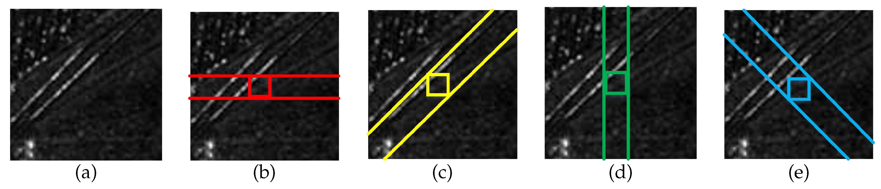
Figure 3.
Framework of attribute learning. Attributes are learned by iteratively repeating clustering and classification procedure.
Figure 3.
Framework of attribute learning. Attributes are learned by iteratively repeating clustering and classification procedure.

Figure 4.
Framework of SAR image classification based on attributes. The first step is low-level features extraction; then, the attributes that appeared in the test image are detected, and the frequency of the detected attributes is described by a statistic histogram; finally, a linear SVM classifier is used to perform classification.

Figure 5.
(a–c) Experimental SAR image acquired by TerraSAR-X in Guangdong, China.

Figure 6.
Five detected patches for each category. The detected patches from (a) to (g) correspond to the categories in Figure 5; those patches among different categories exhibit distinct visual properties, whereas five patches within each category demonstrate remarkable resemblance.
Figure 6.
Five detected patches for each category. The detected patches from (a) to (g) correspond to the categories in Figure 5; those patches among different categories exhibit distinct visual properties, whereas five patches within each category demonstrate remarkable resemblance.


Table 1.
Parameters for attribute learning.
| Parameter Index | Setting |
|---|---|
| patch size | from pixels to global size with 3 pixels shift |
| stride | 3 pixels |
| number of sampled patches | n |
| initial cluster center | |
| members forming final cluster center |
Table 2.
Performance comparison in terms of accuracy, average accuracy, Kappa coefficient and associated confidence interval.
Table 2.
Performance comparison in terms of accuracy, average accuracy, Kappa coefficient and associated confidence interval.
| Class/Method | GLCM | Gabor | GMRF | PFST | BoW-MV | AL |
|---|---|---|---|---|---|---|
| Forest | 78.33 | 53.33 | 86.67 | 79.00 | 80.12 | 92.37 |
| Hill | 78.33 | 28.33 | 68.33 | 81.00 | 39.13 | 81.45 |
| Industrial area | 55.00 | 50.00 | 46.67 | 63.00 | 59.01 | 78.66 |
| Farmland | 90.00 | 80.00 | 98.33 | 99.00 | 83.23 | 96.34 |
| River | 100 | 95.00 | 100 | 79 | 92.55 | 98.60 |
| Urban area | 70.00 | 30.00 | 68.33 | 100 | 75.78 | 92.66 |
| Others | 61.67 | 68.33 | 71.67 | 77.00 | 72.67 | 72.88 |
| A.A. | 76.19 | 57.86 | 77.14 | 82.57 | 72.61 | 89.27 |
| Kappa | 0.72 | 0.51 | 0.73 | 0.80 | 0.67 | 0.86 |
| Kappa C.I. | [0.67,0.77] | [0.45,0.56] | [0.69,0.78] | [0.79,0.80] | [0.66,0.67] | [0.83,0.89] |
© 2017 by the authors. Licensee MDPI, Basel, Switzerland. This article is an open access article distributed under the terms and conditions of the Creative Commons Attribution (CC BY) license (http://creativecommons.org/licenses/by/4.0/).
Share and Cite
MDPI and ACS Style
He, C.; Liu, X.; Kang, C.; Chen, D.; Liao, M. Attribute Learning for SAR Image Classification. ISPRS Int. J. Geo-Inf. 2017, 6, 111. https://doi.org/10.3390/ijgi6040111
AMA Style
He C, Liu X, Kang C, Chen D, Liao M. Attribute Learning for SAR Image Classification. ISPRS International Journal of Geo-Information. 2017; 6(4):111. https://doi.org/10.3390/ijgi6040111
Chicago/Turabian StyleHe, Chu, Xinlong Liu, Chenyao Kang, Dong Chen, and Mingsheng Liao. 2017. "Attribute Learning for SAR Image Classification" ISPRS International Journal of Geo-Information 6, no. 4: 111. https://doi.org/10.3390/ijgi6040111
Note that from the first issue of 2016, this journal uses article numbers instead of page numbers. See further details here.