
Forecasting Urban Vacancy Dynamics in a Shrinking City: A Land Transformation Model

Department of Landscape Architecture and Urban Planning, Texas A&M University, College Station, TX 77843, USA
*
Author to whom correspondence should be addressed.
ISPRS Int. J. Geo-Inf. 2017, 6(4), 124; https://doi.org/10.3390/ijgi6040124
Submission received: 28 February 2017
/
Revised: 14 April 2017
/
Accepted: 16 April 2017
/
Published: 20 April 2017
Abstract
:In the past two centuries, many American urban areas have experienced significant expansion in both populating and depopulating cities. The pursuit of bigger, faster, and more growth-oriented planning parallels a situation where municipal decline has also been recognized as a global epidemic. In recent decades many older industrial cities have experienced significant depopulation, job loss, economic decline, and massive increases in vacant and abandoned properties due primarily to losses in industry and relocating populations. Despite continuous economic decline and depopulation, many of these so-called ‘shrinking cities’ still chase growth-oriented planning policies, due partially to inabilities to accurately predict future urban growth/decline patterns. This capability is critical to understanding land use alternation patterns and predicting future possible scenarios for the development of more proactive land use policies dealing with urban decline and regeneration. In this research, the city of Chicago, Illinois, USA is used as a case site to test an urban land use change model that predicts urban decline in a shrinking city, using vacant land as a proxy. Our approach employs the Land Transformation Model (LTM), which combines Geographic Information Systems and artificial neural networks to forecast land use change. Results indicate that the LTM is a good resource to simulate urban vacant land changes. Mobility and housing market conditions seem to be the primary variables contributing to decline.
1. Introduction
Today, the world is undergoing the largest wave of urban growth in history. Global populations are projected to increase by 2.3 billion by 2050, with urban populations rising from 3.6 billion to 6.3 billion (nearly 67% of the world’s population) [1,2]. This trend will not be evenly disturbed, however, as not all cities will absorb this population growth; this uneven distribution will contribute to the induction of significant social, economic, and environmental changes [3]. In recent decades, many former industrial cities have experienced serious depopulation, job loss, and economic decline due to loss of industry and out-migrating younger populations; these cities are known as shrinking cities. Unfortunately, despite continuous economic decline and depopulation, many shrinking cities still chase growth-oriented urban design and planning goals due to the inability to accurately predict future urban growth patterns.
While the term shrinking city has been widely used, definitions and measurements of urban shrinkage have been differently categorized depending on the purpose of studies and/or research. In sum, a shrinking city can be defined as a non-growing city that has diluted urban physical, social, and environmental functions due to the loss of population, slowdown in economic growth, and deterioration of urban infrastructure [4,5,6,7]. The most visible byproduct of urban shrinkage is vacant and abandoned property; vacant land represents the physical manifestation of economic decline, and, consequently, the growing amount of these properties has emerged as a critical theme to measure the effects of urban shrinkage [8,9,10].
To better understand the geographical dynamics of vacant properties in shrinking cities, a growing number of recent studies has sought to quantify the extent of their influence. Most of this research has identified the number of vacant properties by cities or by region, but failed to do longitudinal assessments or develop comprehensive factors to predict spatial and temporal changes simultaneously. Historically, this was primarily due to insufficient databases and a lack of development in computer technology.
This research develops a model to accurately predict urban decline in shrinking cities, using vacant land as a measure. The research analyzes vacant land patterns in the city of Chicago, Illinois, USA over the past 20 years, and verifies the analytical and technical capabilities of using a Land Transformation Model (LTM) to predict future vacant land. In most land use prediction studies, there is a lack of explanation of the influences of predictor variables and insufficient testing of the accuracy assessment of the prediction output. To fill this gap and increase model output validity and reliability, this research performs four different accuracy assessment processes: kappa coefficients, percent correct metric (PCM), agreement/disagreement measures, and the relative operating characteristic (ROC).
2. Literature Review
2.1. Definition of Vacant Land
There are many ways to define vacant land; it can be defined by municipality, situation, duration of vacancy, and/or function of parcel. In some cases, only urban lots deemed unsafe or difficult to develop are designated as vacant land. However, brownfields or abandoned parcels including dilapidated residential, commercial, or industrial buildings/sites are also sometimes considered vacant land. Furthermore, in some studies vacant land has also included open space such as parks, farm sites, and properties with particular natural resource value [11].
Vacant land includes not only empty or underperforming areas, but also abandoned and neglected industrial buildings that may pose a threat to public safety. The National Vacant Properties Campaign (NVPC) defines a property as vacant if one or both of the following characteristics is met: (1) “the site poses a threat to the public”, or (2) “the owners or managers neglect the fundamental duties of property ownership (e.g., they fail to pay taxes or utility bills, default on mortgages, or carry liens against the property.)” (p. 1, [12]). Based on this definition, vacant properties include not only under-performing industrial buildings and lots (brownfields), but also residential and commercial properties (greyfields) that have been unoccupied or beyond repair over a year. Due to oversupplies of urban vacant land, property owners in neighborhoods having large amounts of vacant lots oftentimes have difficulty re-selling and suffer losses in the market value of their properties. Consequently, decreasing tax revenues from reduced property values can make it difficult for the city to perform public improvements and maintenance on these sites [8].
Vacant or neglected properties are not always a bad thing, and they do not always have to be damaged or derelict. Some types of vacant land are unused but can be productive. Some may have natural resource value for inhabitants and provide green space such as park space or green infrastructure. Once a city has too much vacant land, it may reflect a long cycle of depopulation and economic downturn. So, a large amount of vacant lots presents a concern in shrinking cities; the difficulty lies in changing them into valued commodities. In contrast, an insufficient amount of vacant land can hinder future growth and development. The primary goal is, therefore, to find the most effective land supply usage [13].
2.2. Causes and Impacts of Vacant and Abandoned Properties
Urban shrinkage is a multi-faceted process created by the interaction of many physical, social, economic, and environmental factors. As neighborhoods decline, vacant properties increase and decreases in property values typically occur. As a result, rental properties may not produce enough income to cover taxes and other related costs, forcing landlords to disinvest in these aging properties. Property owners may wish to sell urban lots that are no longer economically viable, but increased housing supplies on the suburban fringe decrease demand for these properties; consequently, it can become nearly impossible to sell them [14,15,16]. Landlords reluctant to maintain or invest in declining properties decrease the ability to attract new tenants. These interrelated consequences make vacant land, the byproduct of urban decline, a causal factor of itself. Increases in vacancies and abandonment produce deterioration and a waste of housing resources, causing more residents to feel unsafe and leave. These vacant and abandonment properties are recognized as problems not only for the property itself but also for entire neighborhoods and local governments in a vicious cycle of decline.
A decline in output and employment in the manufacturing sector can also be a primary factor contributing to urban shrinkage. The weakened industrial competitiveness of traditional U.S. industries (e.g., steel and iron manufacturing) has led to both reduced demand for unskilled or low-skilled laborers and decreasing income levels of workers dependent upon these industries. Consequently, unstable financial situations due to long-term unemployment and an increase in non-regular workers have shaken and destabilized many shrinking communities and created a situation where affluent skilled laborers leave the city and only the people who cannot afford to move stay.
Growing amounts of vacant and abandoned properties threaten neighborhood stability. As properties decay, they can be used for violent crime or be targets of vandalism [15,17,18,19]. Increased vacancy rates and violent crime levels contribute to lower residential satisfaction and result in lower rents or housing prices, and consequently, lead to a growing number of residents’ decisions to move out. Spelman [19] found that 41% of abandoned residential buildings are unsecured and 83% are used for illegal activities in a low-income neighborhood in Austin, Texas, USA. More recently, Cui & Walsh [17] and Immergluck and Smith [15] also examined the relationships among foreclosure, vacancy, and crime. They found that many abandoned unsecured residential properties are used for illegal activities. According to the research, once foreclosed properties become vacant, violent crime rates can increase by more than 15% [18].
In spite of attempts by local governments to manage the decline, the number of vacant properties has grown rapidly in many shrinking cities. According to a survey conducted by the U.S. Government Accountability Office in 2011, most shrinking cities spent a majority of their investments on boarding up and cleaning vacant properties. For example, Chicago spent $875,000 on 627 properties, Detroit spent $1.4 million on 6000 properties, and Baltimore spent over $2 million each year [18]. In spite of these investments, research also found that there is an increased financial burden on local governments to maintain public infrastructure; there is an annual increase of $1427 for each vacant property for police and fire services, on average [18].
2.3. The Land Transformation Model
In an effort to assist in solving many of the aforementioned urban issues, planners have slowly moved to spatial and temporal models that are more scientifically and technologically driven. The LTM, one such model, is a Geographic Information Systems (GIS) and artificial neural networks (ANNs) based land use/cover change (LUCC) model that has recently grown in popularity for analyzing spatial and temporal land use dynamics, estimating the impacts of urban growth alterations, and forecasting land use changes [20,21]. GIS tools are used to process and manage spatial data layers, while ANNs learn about input patterns (driving factors) and output data (historical land use change) [22]. The LTM was originally developed by the Human-Environment Modeling and Analysis Laboratory at Purdue University to simulate future land use change over regions and measuring the environmental and economic impacts of urbanization and agricultural expansion. Since a variety of input factors including physical, socioeconomic, political, and environmental variables can be used for predicting future land use change, the LTM can provide valuable information about the potential effects of land use change in diverse fields such as forest cover change and urban environments [22,23,24].
The LTM’s ability to successfully simulate land use changes has increased its utility on a multitude of scales/locations [25]. It was developed over 15 years ago and has now been utilized in a variety of places around the world [22]. Brown, Pijanowski, and Duh [26] used the model to predict regional forest cover changes in the Upper Midwest, USA, using multiple socioeconomic, human-induced drivers; results showed that land use and land cover were linked and linear functional relationships between the two were established through regression analysis. Tang et al. [27] investigated urbanization patterns on a watershed scale and forecasted land use change by 2020 and 2040 using the LTM. As a tool of environmental impact assessment, the research used the model to generate information about future urbanization patterns and estimate potential environmental impacts. Similarly, the LTM was used to examine the impacts of land use morphology on environmental processes by Ray and Pijanowski in 2010 [28]. The model has also recently been coupled with meso-scale drivers to project urban growth using multiple city-scaled projections combined and assessed on a national scale [20]. Tayyebi et al. [24] forecasted civic boundary expansion in an effort to control for urban growth, finding that LTM models performed relatively well using this method and that the introduction of small-scale data into large-scale LTM simulations significantly increased the model accuracy.
As noted, urban land use change models have been widely used in various areas. However, despite continuous economic decline and depopulation, shrinking cities are still hindered by an inability to accurately predict future urban decline patterns, specifically with regards to vacant land accumulation. As such, the current urban challenge should not concentrate on simply projecting urban development, but finding ways to analyze land use changes and manage vacant land as a resource that can be beneficial to local communities socially, physically, and environmentally [10,29]. More accurate and proactive land-use planning mechanisms may be more effective than reactive policies in dealing with the vacancy issue [30]. Relatedly, the LTM is a good spatial solution for analyzing historical urban land-use changes, forecasting future possible situations, and simulating policy scenarios [20]. This research both develops and uses causal drivers to predict future vacant land in shrinking cities; the findings are useful for more accurately simulating land use changes to suggest suitable alternatives for cities experiencing urban decline.
3. Literature Gaps and Research Objectives
A multitude of LUCC models have been developed over the last 50 years in diverse fields including urban planning, geography, statistics, and computer science, ranging from statistical and econometric models to GIS-based models. Many researchers and professionals have used diverse land use change models to explore the drivers and patterns of land use change, to make possible future scenarios and to provide appropriate policies affecting the changes by analyzing the causes and consequences of land use changes [31,32,33,34,35]. Most existing land use change models, however, have been criticized for not being able to provide reliable accuracy assessment processes of the output effectively [36]. Since doubt and questions about the outputs still remain, the models can have difficulties adapting to local circumstances due to reliability and accuracy issues [37]. In order to improve the modeling capability, it is critical to utilize a series of accepted assessment methods to increase and validate model accuracy. Furthermore, while most LUCC models are used to predict urban growth patterns, there is only limited research about a singular model specifically targeting vacant land use patterns at the local, municipal scale. Although Newman et al. [20] dealt with the vacancy issue in a growing city (Fort Worth, Texas, USA), no models have been created that specifically target vacant land uses for shrinking cities; no one has yet used the LTM to predict urban decline. Vacant parcels are used as a proxy for measuring and assessing urban decline [9,20,38,39,40]. Therefore, the main purposes of this research are twofold: (1) to forecast future possible spatiotemporal vacancy scenarios utilizing driving factors influence on historical vacancy dynamics in cities that have suffered chronic vacancy issues, and (2) to develop a methodological framework to simulate urban decline and vacant land pattern change in shrinking cities, which is validated using proven methods of calibration.
4. Materials and Methods
4.1. Study Area and Data
The city of Chicago in Cook County, Illinois is utilized as the study area and spatiotemporal datasets in a spatial geographic format are required to conduct this research. The time span of analysis is 20 years, covering a time frame from 1990 to 2010. The Chicago Metropolitan Agency for Planning (CMAP) provided the land use and vacant land inventory data in GIS format in 10-year intervals from 1990 for the entire Chicago metropolitan area. Therefore, this study utilizes the definition of vacant land by CMAP. They define vacant land as land in an undeveloped state, with no agricultural activities nor protection as open space [41], and categorize it into four different classifications: (1) brownfields, (2) vacant structures/housing units, (3) under development/construction and (4) vacant forested, grassland and wetlands. Vacant brownfields are described as underutilized, obsolete, or structurally deteriorated industrial or commercial properties where improvements are hindered by real or perceived contamination. Vacant structures/housing units contain undeveloped land classified as residential, commercial, and industrial by the county assessor. Under development/construction is described as land with construction activities in aerial imagery (i.e., roadway begun, partially completed structures, missing or incomplete landscaping). Vacant forested, grassland, and wetlands describes grassland or wetlands with more than 2.5 acres.
In 2000, 62 cities in the United States had a population of over 250,000 (excluding Honolulu, HI). Among them, the city of Chicago lost 200,418 people (−7%), the second largest loss after Detroit (−237,493 or −25%) during the same time period (Table 1). In spite of Chicago’s depopulation rate, decline-related issues in the city have been relatively overlooked compared to other shrinking cities such as Detroit, Cleveland, and Baltimore. Chicago experienced rapid population growth until the 1950s. As early as 1947, manufacturing factories began to move from the urban area into the suburbs. By 1980, the U.S. Census showed that of the 16 poorest neighborhoods in the country, 10 were located in Chicago [42]. By 2010, Chicago had lost around 925,300 people from the 1950 population peak, reporting a 6.9% decrease between 2000 and 2010. The U.S. Census Bureau projected Chicago would lose more than 1 million people between 1950 and 2020, which only two municipalities worldwide have ever experienced: London and Detroit [43]. The city also faced a high unemployment rate during this time (11.2%), ranking 11th among the 50 largest cities in 2010. Furthermore, per capita income in Chicago ($28,000) was only 70% of the national average of $40,000 [44].
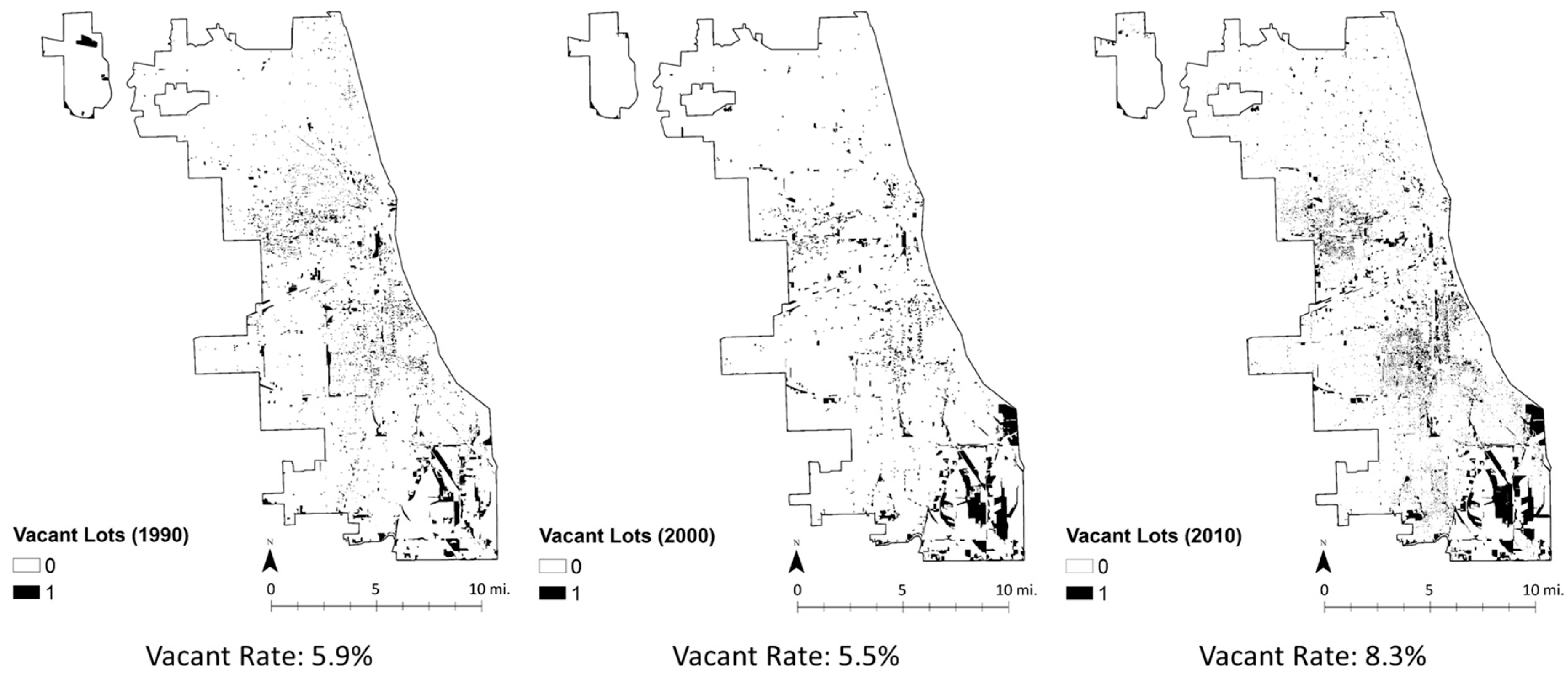
Figure 1 shows vacant land patterns and ratios of vacant land in Chicago between 1990 and 2010 in 10-year increments based on the definition of vacant land by CMAP. As shown in the figure, as the population of the city became more stable by the 1990s and early 2000s, the total amount of vacant land in Chicago dropped by 0.4%, to about 5.5%. However, Chicago increased in vacant land by 2.8% from 2000 to 2010, with a large majority of current vacant parcels residing in the city’s core and manufacturing/industrial neighborhoods in the southeast. Like many older industrial cities in the USA, Chicago has also suffered from a growing number of vacant and abandoned lots. This condition was more recently exacerbated due to the national foreclosure crisis in 2008 and other depopulation trends characterizing its surrounding region. The city lost over 200,000 people from 2000 to 2010; this negative population growth contributed to increases in vacant land. Chicago had 33,902 vacant homes in 2013, an increase of 22% from 2010. Regionally, suburban Cook County had 21,479 vacant homes, up 79% from 2010, and a vacancy rate over 17% in some census tracts in South Side neighborhoods, according to [45].
4.2. Variable Selection
Because spatial prediction outcomes are greatly affected by variable selection, identifying which factors determine vacant land formation/accumulation is critical to output accuracy. Several studies have identified principal causal mechanisms contributing to vacant urban land, but studies that quantify the exact influence on vacant land accretion are difficult to find [20]. The primary causes of vacant land can be categorized by four different, yet overlapping, classifications: (1) deindustrialization or shifts from an industrial to service economy [40,46,47,48], (2) weak market conditions and downturns [49,50,51], (3) decreasing personal wealth [52,53,54], and (4) odd physical characteristics/bad location [40,53,55]. Due to these factors, losses in residential, commercial, and business activities due to an oversupply of vacant land can, in many cases, result in a decrease in land prices, property values, and tax revenues [7,56]. With this in mind, 18 appropriate input factors that contribute to vacant land were selected as drivers to predict urban decline, based on evidence derived from the literature. Depending on the data capability from each time frame assessed, these models used 16 to 18 input factors. Table 2 shows each input factor by the year it was examined, a description, and the previous research that utilized it as a causal driver for vacant land formation. Socioeconomic variables such as poverty, educational attainment, and unemployment rate were collected from the U.S. Census Bureau at the census block group and parcel levels (parcel size); transportation data (proximity to highways and railroads) were provided by the City of Chicago’s Geographic Information System. Then, vacant land inventories and factor data were rasterized at a resolution of 100 × 100 ft.
Employment trends such as unemployment rate and secondary industry quotient are typically noted as primary causes of vacant land [42,57,58]. Since 2000, more than five million manufacturing jobs have disappeared in the USA. While about 24% of American workers were employed in manufacturing in 1960, only about 8% of American workers have a job in the sector today [59]. The devastation of most American manufacturing cities, particularly in the Midwest, is a testament to this decline. Fee and Hartley [56] found that declining Metropolitan Statistical Areas (MSAs) had a large concentration of employment in manufacturing industry, an average of 30%, while the manufacturing industry rate in other MSA was less than 20% in the 1980s. As such, MSAs with the heaviest historic concentration of manufacturing jobs have a much higher rate of depopulation and economic decline than the average MSA; simultaneously, the growth of service industries tends to attract people to cities [58]. Thus, it was assumed that higher unemployment rates and secondary industry rates would increase vacant land.
Factors associated with individual personal wealth and socioeconomic status such as poverty rate, income level, and level of educational attainment are also highly associated with urban shrinkage and increases in vacant land. Mallach & Brachman [60] found that the poverty level of eight shrinking cities in Ohio was about twice as high as the national average (of 13.2%). Unstable financial situations due to weakened industrial competitiveness and long-term unemployment destabilized many communities. Furthermore, some research revealed that the percentage of adults who hold a bachelor’s degree or higher is the most critical tool in measuring a city’s social and economic wellbeing, and that a higher level of education is a critical growth engine for population and income growth in cities [61,62].
Racial segregation has also been found to be associated with an increase in vacant properties. Over time, widespread racial discrimination, seen in hiring and housing market trends, has systematically limited relocation options for many minority populations [63,64]. When a neighborhood loses jobs, minorities have fewer housing choices, further increasing the minority concentration in these areas [65]. Fee and Hartley [58] investigated demographic changes within 36 MSAs experiencing depopulation between 1980 and 2010 and found that, in spite of drops in total population density during the time, the fraction of minority residents increased mostly within 10 miles of the CBD [58].
Housing quality and homeownership are also clearly defined as factors contributing to an increase in vacant and abandoned properties. The national residential housing vacancies and homeownership report by the Census Bureau [66] found that the rental housing vacancy rate (6.9%) in the fourth quarter of 2016 was about four times higher than that of homeowner housing (1.8%). As Hollander [65] indicated, analysis of occupied housing unit density is an important measure of the physical changes in a city. Since neglected properties might be a sign to communities that there is a lack of neighborhood support, high vacancy rates and lower housing values in a neighborhood can increase the vacancy rates in an entire city. Moreover, when rental properties do not produce enough income to cover taxes and other related costs, it forces landlords to disinvest in aging properties and their ability to attract new tenants decreases.
Parcel size is also a proven factor that can contribute to increases in vacant land. Small/irregularly shaped parcels are sometimes unable to be developed and referred to as leftover/remnant properties [20,67]. Since it can be difficult to sustain functional use in these lots due to physical constraints, this model assumed that smaller parcel size would contribute to increases in vacant land. Parcels less than 5000 ft2 were selected as remnant parcels that contribute to vacant land accumulation.
The massive highway and road construction characterizing the mid-20th century drastically enlarged the size of the geographical area in which people could both live and work [68]. A growing number of people who have left urban areas now commute suburb-to-suburb rather than into the city. Since healthy transportation systems can improve the amenity value of a site by establishing the efficient movement of goods and providing options for people to get to various activities, the accessibility to urban services affects development patterns. Thus, it was assumed that sites nearer to existing major transportation lines would result in decreased vacant land.
4.3. Methodology
4.3.1. LTM
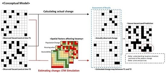
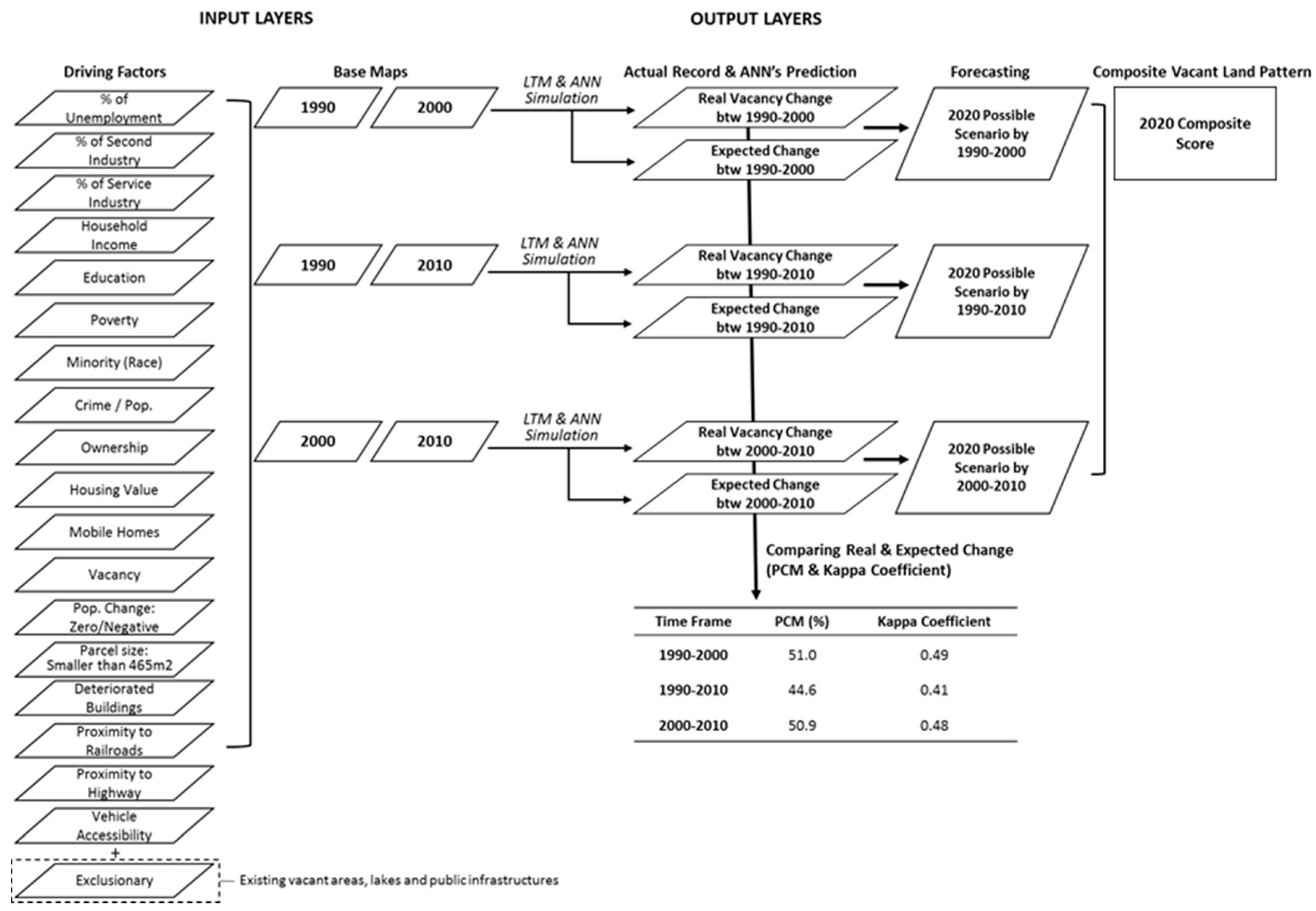
Two different types of input drivers were used to forecast vacant land by 2020 using the LTM: raster-based causal variables linked to a spatial location including socioeconomic data (referred to as input factors) and raster-based historical vacant land use inventories for two different time frames (referred to as input patterns) [20]. Between 16 and 18 different causal variables were chosen as input factors, each of which has been shown to increase vacant land. Then, five different types of land use were omitted from the analysis (referred to as exclusionary layers) due to their specialized functionality (e.g., military bases, airports, public facilities, parks and open space, and existing vacant areas). Using the rasterized input drivers and exclusionary layers, the LTM forecasted three possible vacant land pattern scenarios: Scenario A, based on 1990–2000; Scenario B, based on 1990–2010; and Scenario C, based on 2000–2010 vacant land data. Figure 2 shows the sequential order of our LTM process: (1) analyzing historical vacant land pattern transformation between three different time frames (1990, 2000, and 2010); (2) producing expected vacant pattern changes using 10-year input patterns and 16 to 19 input factors; (3) measuring prediction accuracy by output statistics between actual vacancy transition and predicted transitions using Kappa, PCM, overall agreement and AUC; and (4) predicting future (2020) vacant land patterns.
4.3.2. Accuracy and Reliability
Although LUCC models have risen in popularity, they can be criticized for not always being able to provide highly reliable accuracy outputs due to the ineffective use of upfront calibration methods [36]. Due to this issue, the models can have difficulty in adapting to local circumstances and communities [37]. In order to have an acceptable model and improve the model’s reliability, it is critical to use proven assessment methods for improving model accuracy. For model calibration, four different sets of metrics are used in this research to verify the goodness of fit of the neural network-based model: Kappa coefficients, percent correct metric (PCM), agreement/disagreement measures, and the relative operating characteristic.
Spatially explicit LUCC models typically begin with a digital map of an initial time and then simulate transitions in order to produce a prediction map for a subsequent time [69]. To stabilize the error level to a minimum value, the ANN is required to be trained over 4000 cycles. For the best output, over 250,000 cycles of training are recommended; for this research, each training session was run for 250,000 cycles. Among the multiple types of ANNs, a multi-layer perceptron (MLP) neural net was used in this research. MLPs consist of three different types of layers: input, hidden, and output. Depending on the different time frames examined, 16 to 18 nodes were assigned to both the input and hidden layers, while one node was made for the output layer. Input layers are a series of processing units connected by neurons, which are responsible for passing information throughout the network and characterized by weights based on positive or negative influence on a predictor variable [70]. They are driven by the logic of the modeler and consist of the variables built into the model, which drive the connecting neurons. These connections work out solutions between inputs (i.e., drivers of change) and outputs (e.g., locations of change occurring between two time periods) using non-linear functions and weights [71].
As a result of the neural network training, the LTM produces two automated statistics, Kappa values and percent correct metric (PCM), every 1000 cycles. The cycle with the highest match rate of a pair of maps from categorical land use datasets (actual change and simulated model) was selected for future prediction purposes and assessment [20,22,23]. Generally, the Kappa statistic is a standard component in the conduction of accuracy assessment for a long period [72]. However, the use of only Kappa can be somewhat limited because the Kappa score is a one-dimensional index that fails to accurately evaluate both quantity and location accuracy in grid cells between the utilized maps [73]. Pontius and Millones [74] recommend using much simpler parameters: disagreement and allocation disagreement. Thus, this study utilizes both Kappa coefficient, PCM and disagreement measures. Moreover, we utilized another quantitative measurement tool, ROC (or AUC) analysis, which compares actual and probable transition maps through sensitivity (true positive rate) and specificity (true negative rate).
By juxtaposing actual and predicted maps, four different values are obtained: 0 = no actual and no predicted transition (true negative), 1 = actual but no predicted (false positive), 2 = no actual but predicted (false negative) and 3 = both real and predicted (true positive). Based on the scores, the four accuracy assessment processes will be briefly explained with an example of a nine-pixel-based map (Figure 3). As noted, the LTM provided two automated statistics, Kappa values and PCM evaluating prediction performance by comparing with actual transition expected transition between time frames. The formulas below show the processes.
Based on the formulas, the Kappa coefficient of the example is 0.1, and PCM is 50%. Generally, a Kappa value between 0.01 and 0.20 indicates slight agreement, and PCM results from 40% to 60% are interpreted as acceptable models [23,25,71,75]. Thus, while the Kappa value indicates that agreement would be too poor to accept, if this was an actual model, this example model might be acceptable when considering the PCM. As shown in the example, the use of only an accuracy assessment process can be somewhat limited. For these reasons, quantity disagreement and allocation disagreement for general map comparison can also sometimes provide additional insight [20,74]:
Quantity disagreement indicates the amount of difference between the actual transition map (A) and the predicted transition map (P). Allocation disagreement describes the amount of spatial difference between the two maps. In this example, since the two maps have the same number of changed and non-changed pixels, there is zero quantity disagreement. In terms of allocation disagreement, the five gray pixels indicate the spatial agreement of A and P, meaning that the A and P maps have the same values in the same location, while four white pixels do not share the same values. Thus, the allocation disagreement is 45% (=). Based on the quantitative disagreement and allocation disagreement, overall agreement is calculated as follows; since more than 85% overall agreement is generally used as a baseline for accuracy to be considered good, the fictitious model provided would not be considered acceptable [74].
Overall Agreement (%) = 100 – (Quantitative Disagreement + Allocation Disagreement) = 100 – (0 + 45) = 55%.
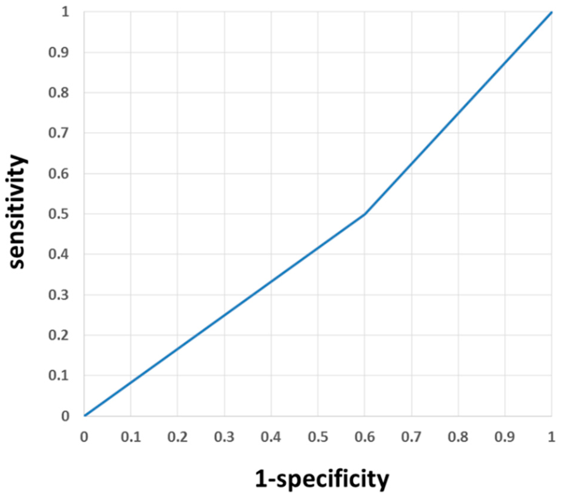
Finally, the receiver operating characteristic (ROC) curve analysis is a quantitative measurement tool to validate the goodness of fit of an LUCC model [20,76,77,78]. Sensitivity (true positive rate) and specificity (true negative rate) are calculated using the formula below, based on the overall agreement cell score outputs. Then, the ROC curve graphs sensitivity on the x on the y-axis against 1-specificity –axis, and the area under the ROC curve (AUC) graphically displays the overall accuracy, as shown in Figure 4. The resulting AUC value for the provided fictitious model is 0.45, meaning that the example model would fail to be acceptable. Typically, values between 0.70 and 0.79 indicate a fair model, 0.80–0.89 substantial, and 0.90–0.99 excellent (1.0 is perfect) [79,80].
5. Results
5.1. LTM Output Statistics
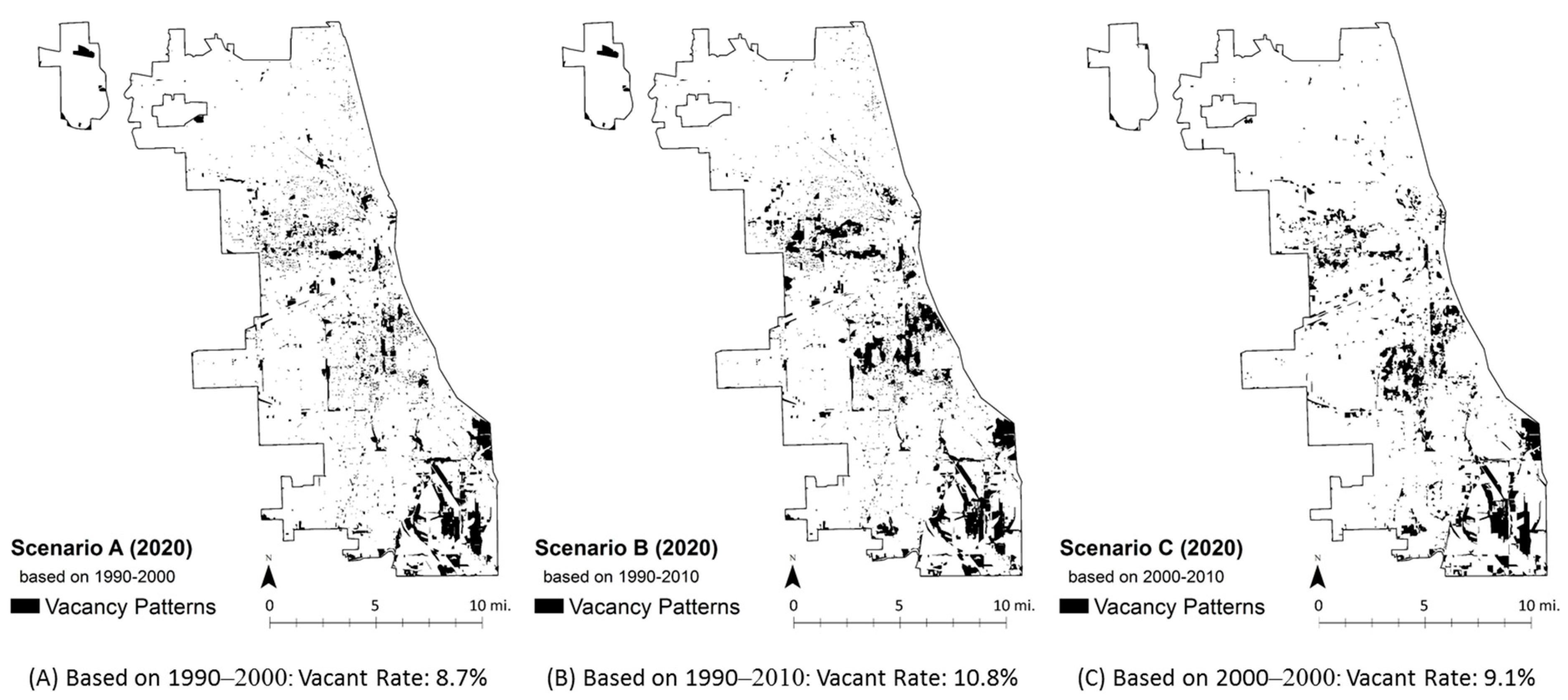
While the above section explains LTM calibration methods using a made-up example, this section reports the output statistics from the Chicago LTM models. In order to forecast future vacant land patterns, spatial patterns and population change between each time period were assessed. For example, the population change between 1990 and 2000 increased by 112,290 (+4.0%), and the number of vacant cells (100 × 100 ft) that transitioned during that time was +2821 (−0.4%). Since the projected population in 2020 is 2,700,000 (decreasing by 196,016 from 2000), cell change was estimated to change at the same rate. Figure 5 shows three different possible scenarios of vacant land in 2020 based on the historical vacant land transformation in three different time frames and 2020 population projections: Scenario A (input patterns from 1990 to 2000), Scenario B (input patterns from 1990 to 2010), and Scenario C (input patterns from 2000 to 2010). As shown in Figure 5, the three scenarios represent similar prediction outputs because vacancy dynamics in the city were fairly stable between 1990 and 2010. The results suggest that most of the vacant land will accumulate in the downtown area and the manufacturing/industrial neighborhoods in the southeast by 2020.
Table 3 shows the output statistics for all models and scenarios trained with the actual population change, number of input factors, the highest probability of each training cycle, and four statistical outputs: Kappa, overall agreement, PCM, and AUC. Overall results from the data produced from LTM show that all scenarios had high enough statistical reliability to merit acceptability of prediction when examining all four methods of accuracy assessment.
Using each prediction map for 2020, a composite score map of all three scenarios was created to find the probability of future vacancy/abandonment. Since each 2020 scenario was given a score of 1 (vacancy) or 0 (non-vacancy), areas where all three scenarios overlapped had a total score of 3. A score of 2 was calculated where two scenarios overlapped, and a score of 1 where only one scenario predicted future vacancy for the parcel (Figure 6). The composite score shows that LTM predicted that 4.2% of the city’s total land area would become vacant in 2020 by all three scenarios, suggesting a high probability of future vacancy/abandonment in these areas. This indicates that all three scenarios shared 29.2% of the predicted vacant area. There was 32.6% (or 4.7% of total land area) overlap for any two scenarios, meaning relatively high probability of future vacancies in these lots, while 38.2% of the predicted vacant land (or 5.5% of total area) was predicted by only one of the given scenarios, suggesting a moderate threat of future vacancy. The composite score output also indicates that the southeast and surrounding downtown areas would have a high risk of vacancy in the future.
5.2. Statistical Vacant Land Clustering: Pattern Density and Hot Spot Analysis
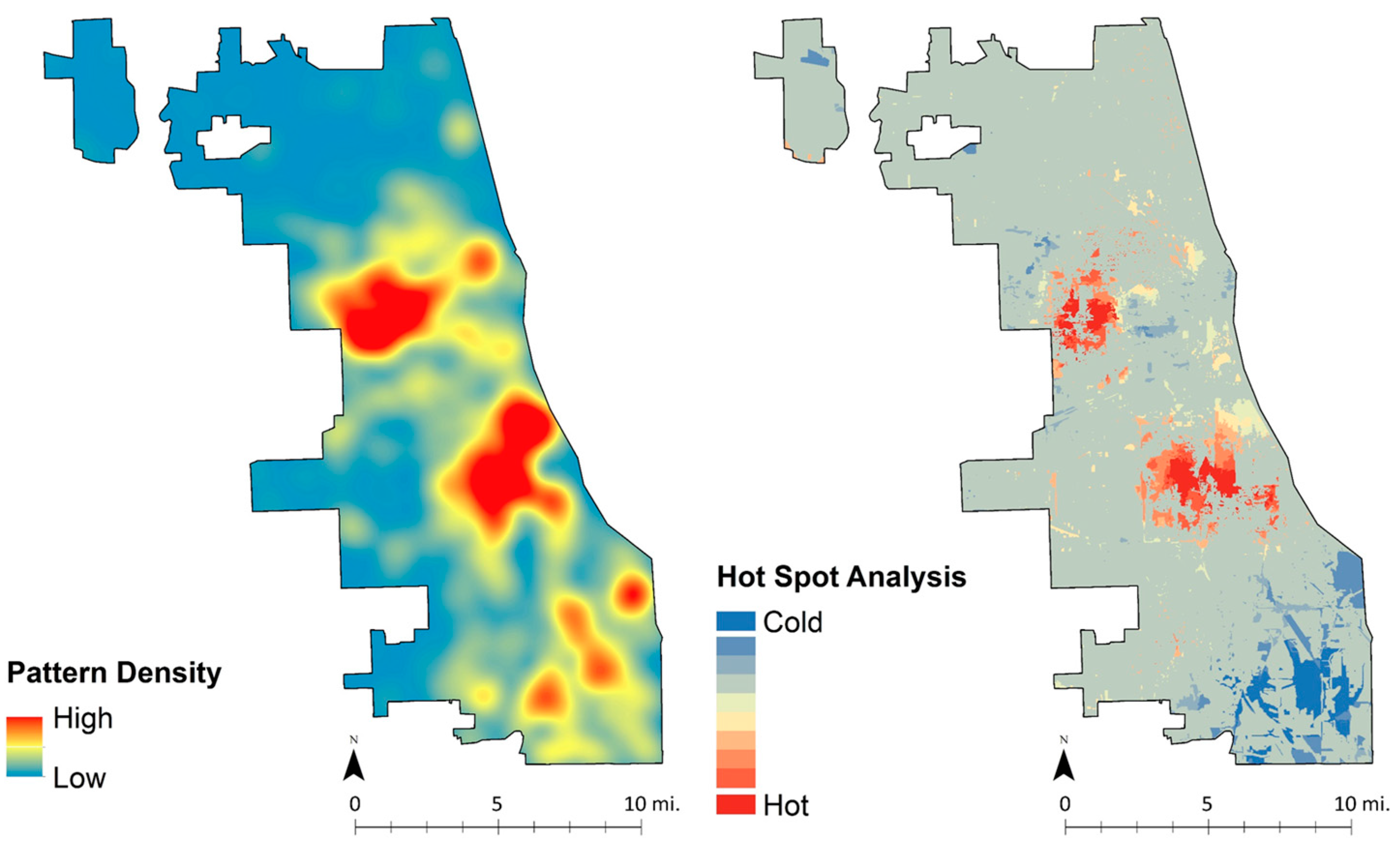
To analyze the statistical clustering of vacant land within the composite score map, pattern density and hot spot analyses were run. Pattern density analysis shows where higher vacant land uses concentrate spatially [20]. The hot-spot analysis tool in GIS is useful to assess statistically significant spatial clusters of high values (hot spots) and low values (cold spots) based on a z-score and p-value—measures of statistical significance indicating whether the observed spatial clustering is more pronounced than one would expect in a random distribution—for each feature examined [81]. The output from these two analyses shows that vacant land will concentrate near the city center and Southeast, while the periphery of the North area has a relatively lower probability of vacancy by 2020 (Figure 7).
6. Conclusions and Discussion
The primary purpose of this research was to test the reliability of the LTM in predicting urban decline in a shrinking city, using vacant land as a proxy. Current conditions require a much better understanding of urban vacancy patterns and methods of assessing the urban condition in shrinking cities [82,83]. Many studies on urban shrinkage have been conducted over the last 20 years. Since the 1980s, GIS has facilitated faster and easier manipulation of spatial datasets, and consequently models are available to predict both temporal and spatial change in land use. However, existing land use change models are criticized due for a lack of objective and scientific frameworks to measure their accuracy. Thus, the research model utilized in this study is designed to establish a more accurate and plausible GIS-based land use change model targeting vacant land use patterns on a local, municipal scale.
Through the spatial accuracy tests of all three scenarios, the LTM proved to be able to assist in targeting sites at high risk of vacancy in the near future. Of course, this is only possible if a clear inventory of vacant land conditions and contributing variables are available. Each model had acceptable Kappa values and PCMs, and there were high enough accuracy outputs of overall agreement and AUC. Policy makers can also modify the driving factors of vacancy to fit the circumstances, and can interpret the simulation results with not only statistical outputs but also intuitive maps and diagrams. Therefore, the ability to generate road maps for local policy makers, developers, and residents who are not familiar with economic theories and statistics makes it much easier to manage possible future urban decline, vacant land, and abandonment.
Land use change models are not perfect due to non-linearity and the realistic complexity of diverse physical, social, and environmental interactions. However, based on qualified theories and relevant data sources, we have shown how vacant land patterns in shrinking cities are likely to change. Thus, we can make more relevant decisions for cities suffering severe depopulation and economic crisis by constructing a rational prediction model. The analysis of causes and consequences of land pattern changes is extremely useful to construct, support, and promote new land use planning policies. Hence, prediction models will play a role as “a key analytical bridge between envisioning alternative urban development patterns and evaluating their impacts” (p. 127, [37]).
This study also has some limitations that should be addressed. First, LTM models must be trained over 250,000 cycles to stabilize the error level for the best output, meaning the process is extremely time-consuming. Longer training times are required for better and more reliable outputs and proper calibration methods to test reliability are even more time-consuming. While cloud-based services such as Geo Planner can, perhaps, speed up this process, model training can be an extreme time constraint. Second, like most LUCC models, the LTM can be influenced by data capability and the classification of land use. Since the definitions and measurements of vacant land differ by city, comparative studies of the amount or transformation of vacant land may be difficult across different cities, and models performed on multiple cities can be plagued by these inconsistent classifications of vacant land. Moreover, since it is impossible to separate the vacant land inventory by different classification types based on the data available, the output may overlook the positive characteristics of certain vacant land types. Lastly, since LTM modeling is a complicated GIS- and ANN-based tool, it may be difficult for those who are not familiar with the tools and extension to apply it to the professional planning field.
Acknowledgments
This research received no specific grant from any funding agency in the public, commercial, or not-for-profit sectors.
Author Contributions
Jaekyung Lee conducted the analysis, pre-processed the data, and wrote the manuscript. Galen Newman substantially contributed to the design of the study, made key suggestions for improving the methods, and edited the manuscript.
Conflicts of Interest
The authors declare no conflict of interest.
References
- Department Economic United Nations. World Population Prospects: the 2012 Revision; Population Division of the Department of Economic and Social Affairs of the United Nations Secretariat: New York, NY, USA, 2013. [Google Scholar]
- Grimm, N.B.; Faeth, S.H.; Golubiewski, N.E.; Redman, C.L.; Wu, J.; Bai, X.; Briggs, J.M. Global change and the ecology of cities. Science 2008, 319, 756–760. [Google Scholar] [CrossRef] [PubMed]
- Grekousis, G.; Mountrakis, G. Sustainable development under population pressure: Lessons from developed land consumption in the conterminous US. PLoS ONE 2015, 10, e0119675. [Google Scholar] [CrossRef] [PubMed]
- Downs, A. Some realities about sprawl and urban decline. Hous. Pol. Debate 1999, 10, 955–974. [Google Scholar]
- Pallagst, K. Shrinking Cities Planning Challenges from an International Perspective Clevelant; Kent State University and Cleveland Urban Design Collaborative: Kent, OH, USA, 2008. [Google Scholar]
- Reckien, D.; Martinez-Fernandez, C. Why do cities shrink? Eur. Plan. Stud. 2011, 19, 1375–1397. [Google Scholar] [CrossRef]
- Schilling, J.; Logan, J. Greening the rust belt: A green infrastructure model for right sizing America’s shrinking cities. J. Am. Plan. Assoc. 2008, 74, 451–466. [Google Scholar] [CrossRef]
- Accordino, J.; Johnson, G.T. Addressing the vacant and abandoned property problem. J. Urban Aff. 2000, 22, 301–315. [Google Scholar] [CrossRef]
- Hollander, J.B.; Pallagst, K.; Schwarz, T.; Popper, F. Planning shrinking cities. Prog. Plan. 2009, 72, 223–232. [Google Scholar]
- Pagano, M.; Bowman, A. Vacant Land as Opportunity and Challenge. In Recycling the City: The Use and Reuse of Urban Land; Lincoln Institute: Cambridge, MA, USA, 2004; pp. 15–32. [Google Scholar]
- Bowman, A.O.M.; Pagano, M.A. Transforming America’s cities: Policies and conditions of vacant land. Urban Aff. Rev. 2000, 35, 559–581. [Google Scholar] [CrossRef]
- Bass, M.; Chen, D.; Leonard, J.; Leonard, J.; Mueller, L.; Cheryl, L.; McCann, B.; Moravec, A.; Schilling, J.; Snyder, K. Vacant Properties: The True Costs to Communities; National Vacant Properties Campaign: Washington, DC, USA, 2005. [Google Scholar]
- Pagano, M.A.; Bowman, A.O.M. Vacant Land in Cities: An Urban Resource; Brookings Institution Center on Urban and Metropolitan Policy: Washington, DC, USA, 2000. [Google Scholar]
- Goldstein, J.; Jensen, M.; Reiskin, E. Urban Vacant Land Redevelopment: Challenges and Progress; Citeseer: Cambridge, MA, USA, 2001. [Google Scholar]
- Immergluck, D.; Smith, G. The impact of single-family mortgage foreclosures on neighborhood crime. Hous. Stud. 2006, 21, 851–866. [Google Scholar] [CrossRef]
- Sternlieb, G.; Burchell, R.W.; Hughes, J.W.; James, F.J. Housing abandonment in the urban core. J. Am. Inst. Plan. 1974, 40, 321–332. [Google Scholar] [CrossRef]
- Cui, L.; Walsh, R. Foreclosure, vacancy and crime. J. Urban Econ. 2015, 87, 72–84. [Google Scholar] [CrossRef]
- Han, H.S. The impact of abandoned properties on nearby property values. Hous. Pol. Debate 2014, 24, 311–334. [Google Scholar] [CrossRef]
- Spelman, W. Abandoned buildings: Magnets for crime? J. Crim. Justice 1993, 21, 481–495. [Google Scholar] [CrossRef]
- Newman, G.; Lee, J.; Berke, P. Using the land transformation model to forecast vacant land. J. Land Use Sci. 2016, 11, 450–475. [Google Scholar] [CrossRef]
- Pijanowski, B.; Shellito, B.; Bauer, M.; Sawaya, K. Using GIS Artificial Neural Networks and Remote Sensing to Model Urban Change in the Minneapolis–St. Paul and Detroit Metropolitan area. Proceedings of American Society of Photogrammetry and Remote Sensing Annual Conference, St. Louis, MO, USA, 23–27 April 2001. [Google Scholar]
- Pijanowski, B.C.; Tayyebi, A.; Doucette, J.; Pekin, B.K.; Braun, D.; Plourde, J. A big data urban growth simulation at a national scale: configuring the GIS and neural network based land transformation model to run in a high performance computing (HPC) environment. Environ. Model. Softw. 2014, 51, 250–268. [Google Scholar] [CrossRef]
- Pijanowski, B.C.; Brown, D.G.; Shellito, B.A.; Manik, G.A. Using neural networks and GIS to forecast land use changes: a land transformation model. Comput. Environ. Urban Syst. 2002, 26, 553–575. [Google Scholar] [CrossRef]
- Tayyebi, A.; Perry, P.C.; Tayyebi, A.H. Predicting the expansion of an urban boundary using spatial logistic regression and hybrid raster–vector routines with remote sensing and GIS. Int. J. Geogr. Inf. Sci. 2014, 28, 639–659. [Google Scholar] [CrossRef]
- Almeida, C.; Gleriani, J.; Castejon, E.F.; Soares-Filho, B. Using neural networks and cellular automata for modelling intra-urban land-use dynamics. Int. J. Geogr. Inf. Sci. 2008, 22, 943–963. [Google Scholar] [CrossRef]
- Brown, D.G.; Pijanowski, B.C.; Duh, J. Modeling the relationships between land use and land cover on private lands in the Upper Midwest, USA. J. Environ. Manag. 2000, 59, 247–263. [Google Scholar] [CrossRef]
- Tang, Z.; Engel, B.; Pijanowski, B.; Lim, K. Forecasting land use change and its environmental impact at a watershed scale. J. Environ. Manag. 2005, 76, 35–45. [Google Scholar] [CrossRef] [PubMed]
- Ray, D.K.; Pijanowski, B.C. A backcast land use change model to generate past land use maps: Application and validation at the Muskegon River watershed of Michigan, USA. J. Land Use Sci. 2010, 5, 1–29. [Google Scholar] [CrossRef]
- Drake, L.; Lawson, L.J. Validating verdancy or vacancy? The relationship of community gardens and vacant lands in the US. Cities 2014, 40, 133–142. [Google Scholar] [CrossRef]
- Park, I.K.; Von Rabenau, B. Tax delinquency and abandonment: An expanded model with application to industrial and commercial properties. Urban Stud. 2015, 52, 857–875. [Google Scholar] [CrossRef]
- Agarwal, C.; Green, G.M.; Grove, J.M.; Evans, T.P.; Schweik, C.M. A Review and Assessment of Land-Use Change Models: Dynamics of Space, Time, and Human Choice; Gen. Tech. Rep. NE-297; U.S. Department of Agriculture, Forest Service, Northeastern Research Station: Newton Square, PA, USA, 2002; 61p.
- Brown, D.G.; Duh, J.D. Spatial simulation for translating from land use to land cover. Int. J. Geogr. Inf. Sci. 2004, 18, 35–60. [Google Scholar] [CrossRef]
- Verburg, P.H.; Schot, P.P.; Dijst, M.J.; Veldkamp, A. Land use change modelling: current practice and research priorities. GeoJournal 2004, 61, 309–324. [Google Scholar] [CrossRef]
- Basse, R.M.; Omrani, H.; Charif, O.; Gerber, P.; Bódis, K. Land use changes modelling using advanced methods: cellular automata and artificial neural networks. The spatial and explicit representation of land cover dynamics at the cross-border region scale. Appl. Geogr. 2014, 53, 160–171. [Google Scholar] [CrossRef]
- Grekousis, G.; Manetos, P.; Photis, Y.N. Modeling urban evolution using neural networks, fuzzy logic and GIS: The case of the Athens metropolitan area. Cities 2013, 30, 193–203. [Google Scholar] [CrossRef]
- Conway, T. The impact of class resolution in land use change models. Comput. Environ. Urban Syst. 2009, 33, 269–277. [Google Scholar] [CrossRef]
- Landis, J.D. Urban growth models: State of the art and prospects. In Global Urbanization; University of Pennsylvania Press: Philadelphia, PA, USA, 2011; pp. 126–150. [Google Scholar]
- Bowman, A.O.M. Terra Incognita: Vacant Land and Urban Strategies; Georgetown University Press: Washington, DC, USA, 2004. [Google Scholar]
- Glaeser, E.L.; Gyourko, J.; Saks, R.E. Urban growth and housing supply. J. Econ. Geogr. 2006, 6, 71–89. [Google Scholar] [CrossRef]
- Németh, J.; Langhorst, J. Rethinking urban transformation: Temporary uses for vacant land. Cities 2014, 40, 143–150. [Google Scholar] [CrossRef]
- Chicago Metropolitan Agency for Planning. 2010 Land Use Inventory: Classification Scheme. Available online: https://datahub.cmap.illinois.gov/dataset/land-use/resource/4102165e-e327-412b-bde2-ebd4a8295f6d (accessed on 27 May 2016).
- Squires, G.D.; Bennett, L.; McCourt, K. Chicago: Race, Class, and the Response to Urban Decline; Temple University Press: Philadelphia, PA, USA, 1989. [Google Scholar]
- Cox, W. The Evolving Urban Form: Chicago. 2011. Available online: http://www.newgeography.com/content/002346-the-evolving-urban-form-chicago (accessed on 2 June 2016).
- U.S. Census Bureau. Chicago City QuickFacts. Available online: https://www.census.gov/quickfacts/map/IPE120213/1714000/accessible (accessed on 21 May 2016).
- Will The Foreclosure Crisis Kill Chicago? Available online: http://www.chicagobusiness.com/article/20131109/ISSUE01/311099980/will-the-foreclosure-crisis-kill-chicago (accessed on 21 February 2016).
- Buhnik, S. From shrinking cities to Toshi no Shukushō: Identifying patterns of urban shrinkage in the Osaka metropolitan area. Berkeley Plan. J. 2010, 23, 132–155. [Google Scholar]
- Lindsey, C. Smart decline. In Panorama: What’s New in Planning; University of Pennsylvania Press: Philadelphia, PA, USA, 2007. [Google Scholar]
- Rieniets, T. Shrinking cities: Causes and effects of urban population losses in the twentieth century. Nat. Cult. 2009, 4, 231–254. [Google Scholar] [CrossRef]
- Bontje, M. Facing the challenge of shrinking cities in East Germany: The case of Leipzig. GeoJournal 2005, 61, 13–21. [Google Scholar] [CrossRef]
- Johnson, M.P.; Hollander, J.; Hallulli, A. Maintain, demolish, re-purpose: Policy design for vacant land management using decision models. Cities 2014, 40, 151–162. [Google Scholar] [CrossRef]
- Ryan, B.D. Design after Decline: How America Rebuilds Shrinking Cities; University of Pennsylvania Press: Philadelphia, PA, USA, 2012. [Google Scholar]
- Audirac, I. Urban Shrinkage Amid Fast Metropolitan Growth (Two Faces of Contemporary Urbanism). 2007. Available online: http://metrostudies.berkeley.edu/pubs/proceedings/Shrinking/10Audirac_PA_final.pdf (accessed on 2 December 2015).
- Cunningham-Sabot, E.; Fol, S. Shrinking cities in France and Great Britain: A silent process. In The Future of Shrinking Cities: Problems, Patterns and Strategies of Urban Transformation in a Global Context; Center for Global Metroplitan Studies: Berkeley, CA, USA, 2009; pp. 17–28. [Google Scholar]
- Rybczynski, W.; Linneman, P.D. How to save our shrinking cities. Public Interest 1999, 135, 30–44. [Google Scholar]
- Henry, M.S.; Schmitt, B.; Piguet, V. Spatial econometric models for simultaneous systems: Application to rural community growth in France. Int. Reg. Sci. Rev. 2001, 24, 171–193. [Google Scholar] [CrossRef]
- Hollander, J.B.; Németh, J. The bounds of smart decline: A foundational theory for planning shrinking cities. Hous. Pol. Debate 2011, 21, 349–367. [Google Scholar] [CrossRef]
- Clark, K.; Drinkwater, S. Enclaves, neighbourhood effects and employment outcomes: Ethnic minorities in England and Wales. J. Popul. Econ. 2002, 15, 5–29. [Google Scholar] [CrossRef]
- Fee, K.; Hartley, D. Economic Trends: Growing Cities, Shrinking Cities. Available online: http://www.clevelandfed.org/newsroom-and-events/publications/economic-trends/2011-economic-trends/et-20110414-growing-cities-shrinking-cities.aspx (accessed on 2 June 2016).
- Long, H.U.S. Has Lost 5 Million Manufacturing Jobs Since 2000. Available online: http://money.cnn.com/2016/03/29/news/economy/us-manufacturing-jobs/ (accessed on 21 January 2016).
- Mallach, A.; Brachman, L. Shaping Federal Policies Toward Cities in Transition: A Policy Brief; Greater Ohio Policy Center: Columbus, OH, USA, 2010. [Google Scholar]
- Glaeser, E.L. A Nation of Gamblers: Real Estate Speculation and American History (Feb. 2013). Am. Econ. Rev. 2013, 103, 1–42. [Google Scholar] [CrossRef]
- Mallach, A. Depopulation, market collapse and property abandonment: Surplus land and buildings in legacy cities. In Rebuilding America’s Legacy Cities: New Directions for the Industrial Heartland; American Assembly, Columbia University: New York, NY, USA, 2012; pp. 85–110. [Google Scholar]
- Massey, D.S.; Denton, N.A. American Apartheid: Segregation and the Making of the Underclass; Harvard University Press: Cambridge, MA, USA, 1993. [Google Scholar]
- Sugrue, T.J. The origins of the urban crisis: Race and Inequality in Postwar Detroit; Princeton University Press: Princeton, NJ, USA, 2014. [Google Scholar]
- Hollander, J.B. Moving toward a shrinking cities metric: Analyzing land use changes associated with depopulation in Flint, Michigan. Cityscape 2010, 12, 133–151. [Google Scholar] [CrossRef]
- U.S. Census Bureau. Quarterly Residential Vacancies and Homeownership, Fourth Quarter 2016. Available online: https://www.census.gov/housing/hvs/files/currenthvspress.pdf (accessed on 12 February 2017).
- Lester, T.W.; Kaza, N.; Kirk, S. Making room for manufacturing: Understanding industrial land conversion in cities. J. Am. Plan. Assoc. 2013, 79, 295–313. [Google Scholar] [CrossRef]
- Rappaport, J. US urban decline and growth, 1950 to 2000. Econ. Rev.-Fed. Reserve Bank Kans. City 2003, 88, 15. [Google Scholar]
- Pontius, R.G.; Boersma, W.; Castella, J.C.; Clarke, K.; de Nijs, T.; Dietzel, C.; Duan, Z.; Fotsing, E.; Goldstein, N.; Kok, K. Comparing the input, output, and validation maps for several models of land change. Ann. Reg. Sci. 2008, 42, 11–37. [Google Scholar] [CrossRef]
- Bishop, C.M. Neural Networks for Pattern Recognition; Clarendon Press: Oxford, UK, 1995. [Google Scholar]
- Pijanowski, B.; Alexandridis, K.; Mueller, D. Modelling urbanization patterns in two diverse regions of the world. J. Land Use Sci. 2006, 1, 83–108. [Google Scholar] [CrossRef]
- Congalton, R.; Mead, R.A. A quantitative method to test for consistency and correctness in photointerpretation. Photogramm. Eng. Remote Sens. 1983, 49, 69–74. [Google Scholar]
- Pontius, R.G. Quantification error versus location error in comparison of categorical maps. Photogramm. Eng. Remote Sens. 2000, 66, 1011–1016. [Google Scholar]
- Pontius, R.G., Jr.; Millones, M. Death to Kappa: birth of quantity disagreement and allocation disagreement for accuracy assessment. Int. J. Remote Sen. 2011, 32, 4407–4429. [Google Scholar] [CrossRef]
- Tayyebi, A.; Pekin, B.K.; Pijanowski, B.C.; Plourde, J.D.; Doucette, J.S.; Braun, D. Hierarchical modeling of urban growth across the conterminous USA: developing meso-scale quantity drivers for the Land Transformation Model. J. Land Use Sci. 2013, 8, 422–442. [Google Scholar] [CrossRef]
- Pontius, R.G., Jr.; Batchu, K. Using the relative operating characteristic to quantify certainty in prediction of location of land cover change in India. Trans. GIS 2003, 7, 467–484. [Google Scholar] [CrossRef]
- Pontius, R.G., Jr.; Si, K. The total operating characteristic to measure diagnostic ability for multiple thresholds. Int. J. Geogr. Inf. Sci. 2014, 28, 570–583. [Google Scholar] [CrossRef]
- Pontius, R.G.; Schneider, L.C. Land-cover change model validation by an ROC method for the Ipswich watershed, Massachusetts, USA. Agric. Ecosyst. Environ. 2001, 85, 239–248. [Google Scholar] [CrossRef]
- Osborne, P.E.; Alonso, J.; Bryant, R. Modelling landscape-scale habitat use using GIS and remote sensing: A case study with great bustards. J. Appl. Ecol. 2001, 38, 458–471. [Google Scholar] [CrossRef]
- Rutherford, G.N.; Bebi, P.; Edwards, P.J.; Zimmermann, N.E. Assessing land-use statistics to model land cover change in a mountainous landscape in the European Alps. Ecol. Model. 2008, 212, 460–471. [Google Scholar] [CrossRef]
- Grubesic, T.H.; Murray, A.T. Detecting Hot Spots Using Cluster Analysis and GIS. In Proceedings of the Fifth Annual International Crime Mapping Research Conference, Dallas, TX, USA, 1–4 December 2001. [Google Scholar]
- Berger, A. Drosscape: Wasting Land Urban America; Princeton Architectural Press: Princeton, NJ, USA, 2007. [Google Scholar]
- Brophy, P.C.; Vey, J.S. Seizing City Assets: Ten Steps to Urban Land Reform. Available online: http://citeseerx.ist.psu.edu/viewdoc/download?doi=10.1.1.148.1390&rep=rep1&type=pdf (accessed on 27 March 2016).
Figure 1.
Historic pattern and ratios of vacant land in Chicago, IL, from 1990 to 2010 in 10-year intervals.
Figure 1.
Historic pattern and ratios of vacant land in Chicago, IL, from 1990 to 2010 in 10-year intervals.

Figure 2.
LTM process diagram showing input factors, input patterns, and output comparison map.

Figure 3.
Diagram showing actual transition, predicted transition, and composite score.
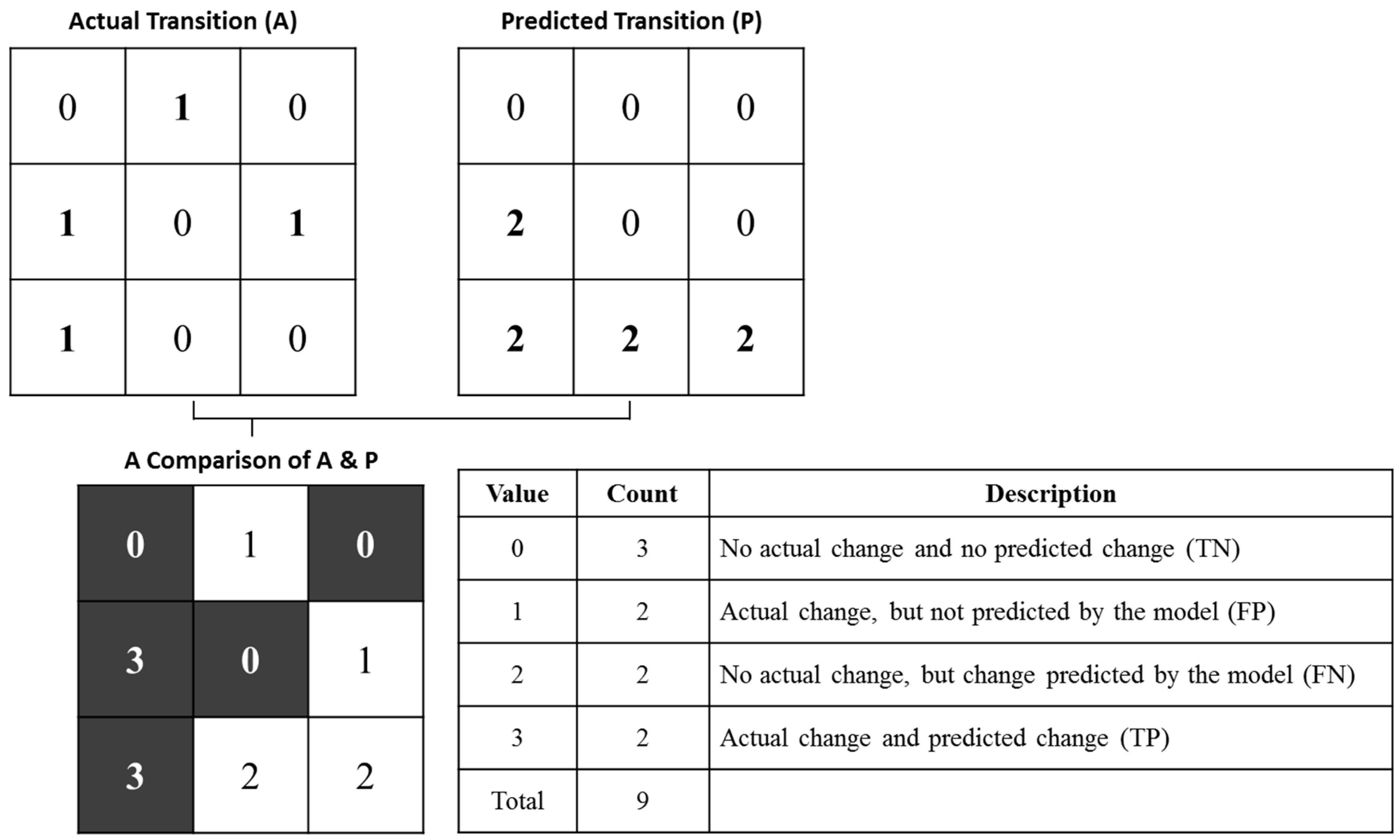
Figure 4.
The AUC output of the example model.

Figure 5.
Possible scenarios of vacancy by 2020 based on (A) 1990–2000, (B) 1990–2010 and (C) 2000–2010.
Figure 5.
Possible scenarios of vacancy by 2020 based on (A) 1990–2000, (B) 1990–2010 and (C) 2000–2010.

Figure 6.
Overlap of all three scenarios for 2020 vacant land predictions in Chicago, IL.
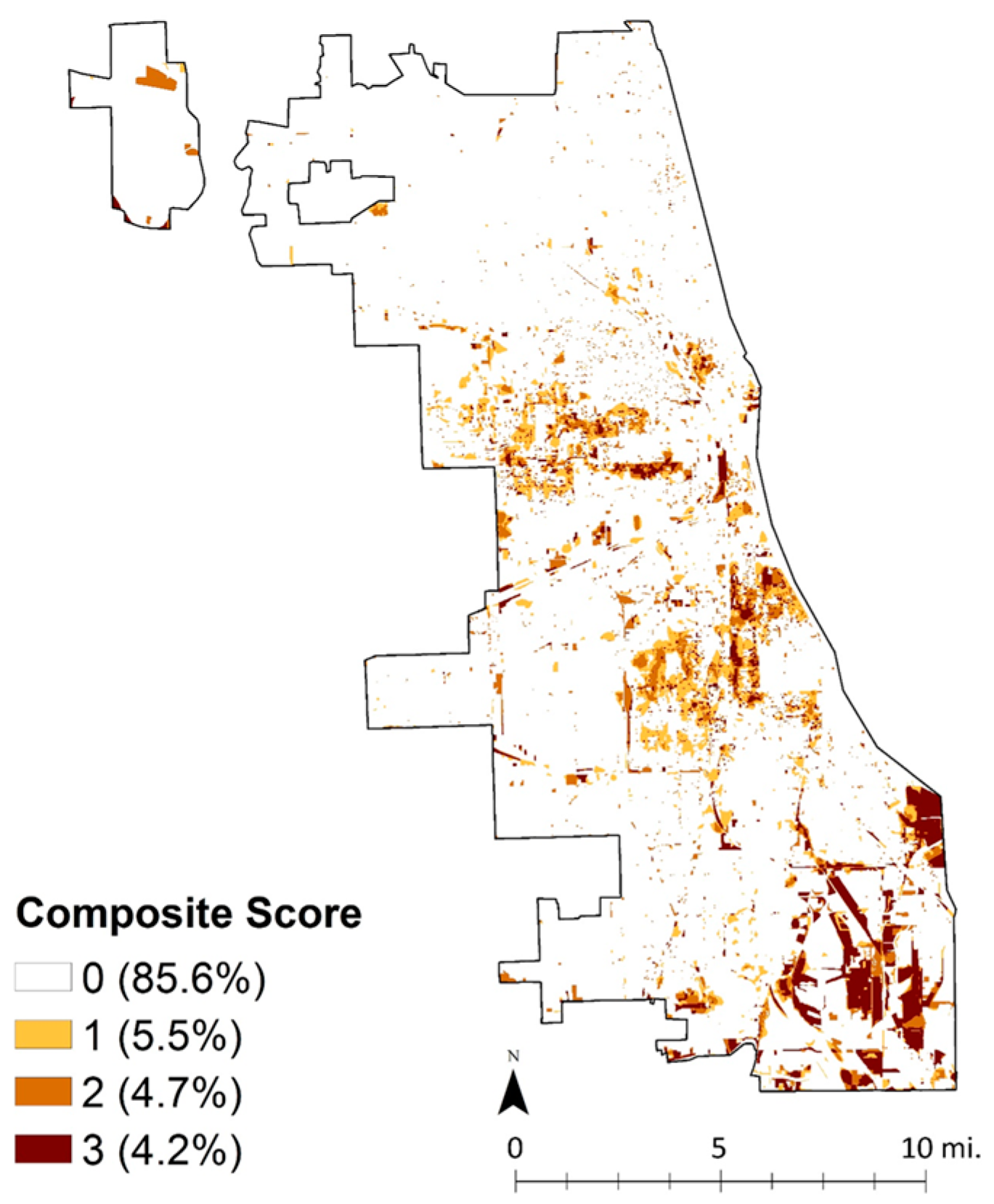
Figure 7.
Vacant land pattern density map (left) and hot-spot analysis showing statistically significant clusters of vacant land (right) in Chicago, IL.
Figure 7.
Vacant land pattern density map (left) and hot-spot analysis showing statistically significant clusters of vacant land (right) in Chicago, IL.


Table 1.
The fastest- and slowest-growing cities by population growth between 2000 and 2010.
| City (State) | Population Change | Population Change (%) | |
|---|---|---|---|
| Top 5 Fastest Growing Cities | Fort Worth (TX) | 206,612 | 39% |
| Charlotte (NC) | 190,596 | 35% | |
| San Antonio (TX) | 182,761 | 16% | |
| New York (NY) | 166,855 | 2% | |
| Houston (TX) | 145,820 | 7% | |
| Top 5 Most Depopulating Cities | Cincinnati (OH) | −34,342 | −10% |
| Cleveland (OH) | −81,588 | −17% | |
| New Orleans (LA) * | −140,845 | −29% | |
| Chicago (IL) | −200,418 | −7% | |
| Detroit (MI) | −237,493 | −25% |
* Since about 29% of the New Orleans population was lost after Hurricane Katrina, the demographic trends of the city may be different from those of cities with a population over 250,000.
Table 2.
Years examined, description, and previous research on input factors utilized as drivers for vacant land prediction.
Table 2.
Years examined, description, and previous research on input factors utilized as drivers for vacant land prediction.
| Input Factors | Input Patterns | U.S. Census Definition | References for Input Factors | ||
|---|---|---|---|---|---|
| 90–00 | 90–10 | 00–10 | |||
| Unemployment Rate | O | O | O | Unemployment rate for civilian population in labor force 16 years and over | Fee & Hartley (2011), Mallach (2012), Aryeetey-Attoh et al. (2015) |
| Service Industry | O | O | O | Proportion of service industry to all industries | Fee & Hartley (2011), Glaeser (2013), Mallach (2012), Lester et al (2013), Glaeser & Kahn (2004), Cochrane et al (2013) |
| Secondary Industry | O | O | O | Proportion of secondary industry to all industries | Fee & Hartley (2011), Mallach (2012), Glaeser (2013), Glaeser & Kahn (2004), Wegener (1982), Dong (2013), Cochrane et al (2013) |
| Household Income | O | O | O | Median household income (Inflation adjusted dollars) | Ryan (2012), Fee & Hartley (2011), Glaeser (2013), Aryeetey-Attoh et al. (2015) |
| Education | O | O | O | Percent of persons 25 years of age and older, with less than or equal to high school graduate (includes equivalency) | Fee & Hartley (2011), Glaeser (2013), Mallach (2012), Parka & Cioricib (2015) |
| Poverty | O | O | O | Individual Poverty Rate: Individuals below poverty=”under 0.50” +“0.50 to 0.74” + “0.75 to 0.99.”) | Ryan (2012), Fee & Hartley (2011), Mallach & Brachman (2010) Glaeser (2013), Parka & Cioricib (2015) |
| Ethnicity | O | O | O | Non-white Population rate to total population | Ryan (2012), Fee & Hartley (2011), Massey and Denton (1993), Sugrue (1996), Hollander (2010) |
| Crime | O | Incidents of crime that occurred in the city | Cui & Walsh (2015). Spelman (1993), Kuo & Sulivan (2001), Jones & Pridemore (2013) | ||
| Home Ownership | O | O | O | Proportion of owner occupied housing units to all occupied housing units | Bradfort (1979), Pond & Yeates (2013), Aryeetey-Attoh et al. (2015), Parka & Cioricib (2015), Hoyt (1993), Temkin & Rohe (1996) |
| Housing Value | O | O | O | Median house value for all owner-occupied housing units | Glaeser & Gyourko (2001), Capozza & Helsley (1989), Dong (2013), Aryeetey-Attoh et al. (2015), Hollander (2010) |
| Mobile Homes | O | O | O | Mobile home rates to all housing units | Glaeser & Gyourko (2001), Hollander (2010), Capozza & Helsley (1989), Dong (2013), Aryeetey-Attoh et al. (2015) |
| Vacancy | O | O | O | Vacancy Rate to all housing units (Occupancy Status) | Mallach (2012), Dong (2013) |
| Population Change | O | O | O | Zero or negative population change between each period | Wegener (1982), Pond & Yeates (2013), Dong (2013) |
| Parcel Size | O | Parcel size smaller than 5000 square foot | Lester et al (2014), Colwell & Munneke (1997), Carrion-Flores & Irwin (2004), Pond & Yeates (2013) | ||
| Age of Buildings | O | O | O | Built before 1950 (except buildings in historical preservation districts) | Wegener (1982) |
| Railroad | O | O | O | Proximity to railroads | Lester et al (2014), Rappaport (2003), Bourne (1996) |
| Highway | O | O | O | Proximity to highways | Lester et al (2014), Rappaport (2003), Bourne (1996), Dong (2013) |
| Accessibility | O | O | O | Proportion of no vehicle available housing units to all occupied housing units | Lester et al (2014), Rappaport (2003), Bourne (1996), Dong (2013) |
| Number of Variables | 16 | 16 | 18 | --- | --- |
Table 3.
LTM statistical output for all models and scenarios trained.
| Input Patterns | Pop. Change | No. of Input Factors | Highest Training Probability | PCM * (%) | Kappa ** | QD (%) | AD (%) | OA *** (%) | AUC **** |
|---|---|---|---|---|---|---|---|---|---|
| 1990–2000 | +112,290 | 16 | 15,000th | 51.0 | 0.49 | 0.0 | 3.7 | 96.3 | 0.70 |
| 1990–2010 | −88,128 | 16 | 100,000th | 44.6 | 0.41 | 0.0 | 6.2 | 93.8 | 0.70 |
| 2000–2010 | −200,418 | 18 | 40,000th | 50.9 | 0.48 | 0.0 | 3.7 | 96.3 | 0.75 |
* PCM: 40–60% is acceptable, ** Kappa: 0.41–0.60 is moderate; *** OA (Overall agreement): more than 85% is considered good. **** AUC: 0.70–0.80 is fair.
© 2017 by the authors. Licensee MDPI, Basel, Switzerland. This article is an open access article distributed under the terms and conditions of the Creative Commons Attribution (CC BY) license (http://creativecommons.org/licenses/by/4.0/).
Share and Cite
MDPI and ACS Style
Lee, J.; Newman, G. Forecasting Urban Vacancy Dynamics in a Shrinking City: A Land Transformation Model. ISPRS Int. J. Geo-Inf. 2017, 6, 124. https://doi.org/10.3390/ijgi6040124
AMA Style
Lee J, Newman G. Forecasting Urban Vacancy Dynamics in a Shrinking City: A Land Transformation Model. ISPRS International Journal of Geo-Information. 2017; 6(4):124. https://doi.org/10.3390/ijgi6040124
Chicago/Turabian StyleLee, Jaekyung, and Galen Newman. 2017. "Forecasting Urban Vacancy Dynamics in a Shrinking City: A Land Transformation Model" ISPRS International Journal of Geo-Information 6, no. 4: 124. https://doi.org/10.3390/ijgi6040124
Note that from the first issue of 2016, this journal uses article numbers instead of page numbers. See further details here.