
A Sparse Manifold Classification Method Based on a Multi-Dimensional Descriptive Primitive of Polarimetric SAR Image Time Series


Abstract
:1. Introduction
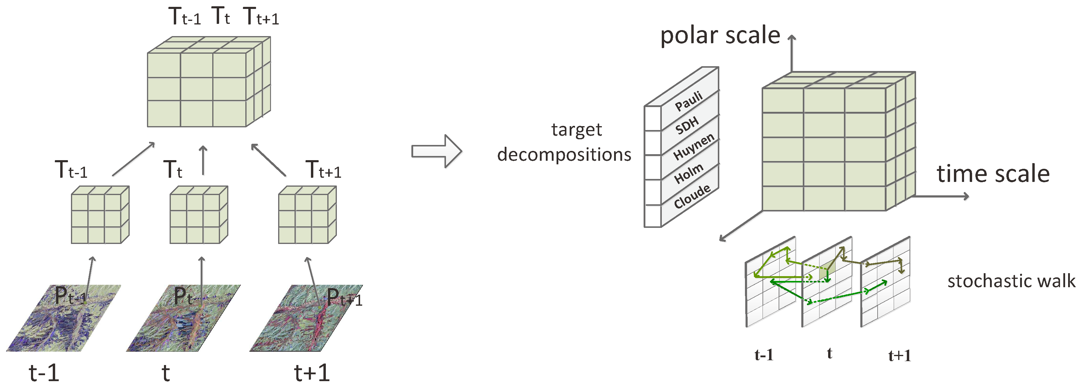
2. The Multi-Dimensional Descriptive Primitive
2.1. Incoherent Feature in the Polarization Scale
2.2. Coherent Feature in the Time Scale
2.3. Multi-Dimensional Descriptive Primitive
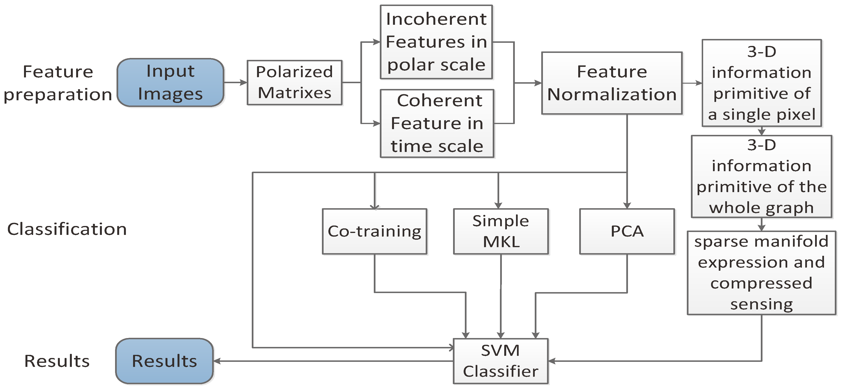
3. The Sparse Manifold Classification Model
3.1. Sparse Manifold Expression
3.2. Compressed Sensing
3.3. Framework
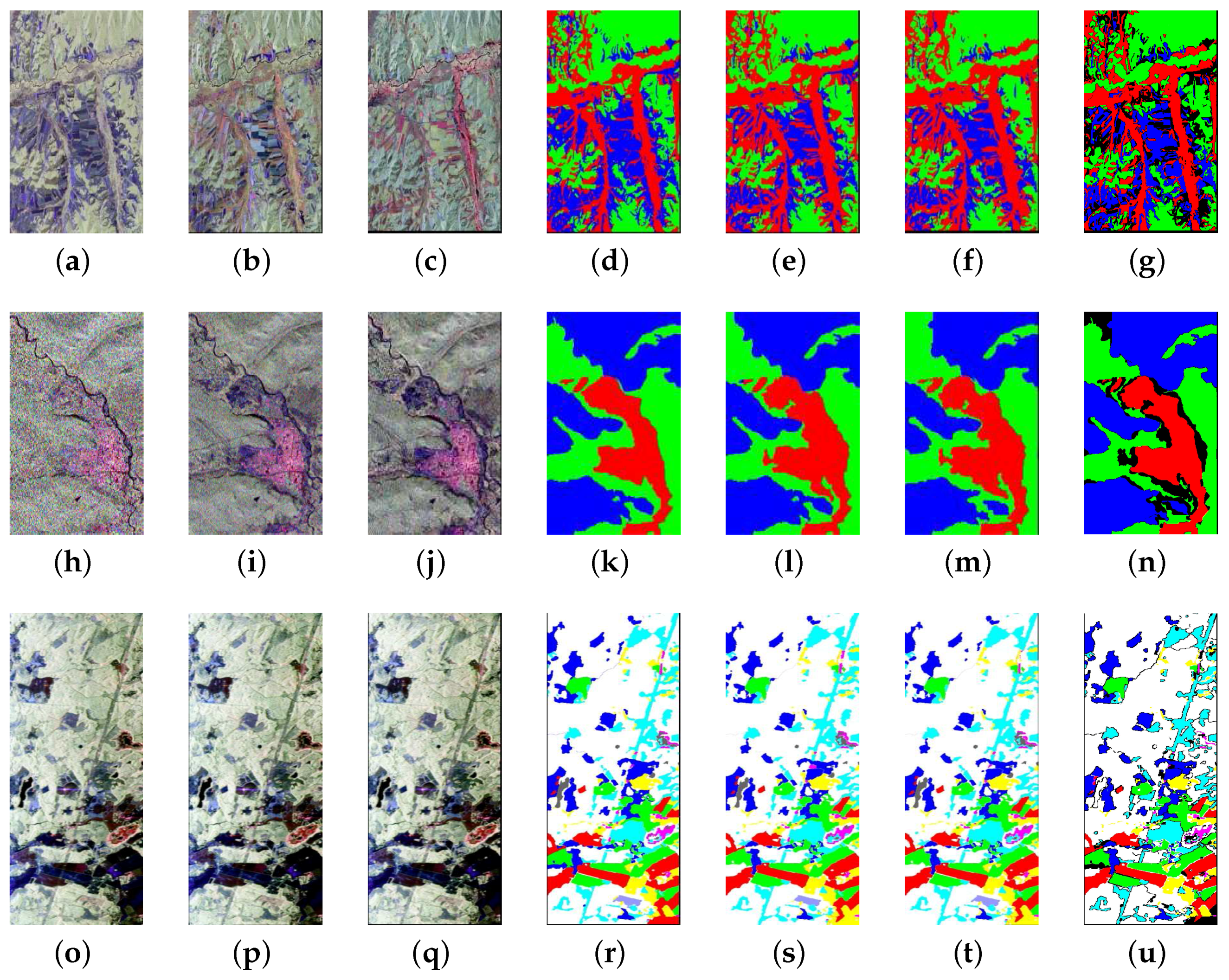
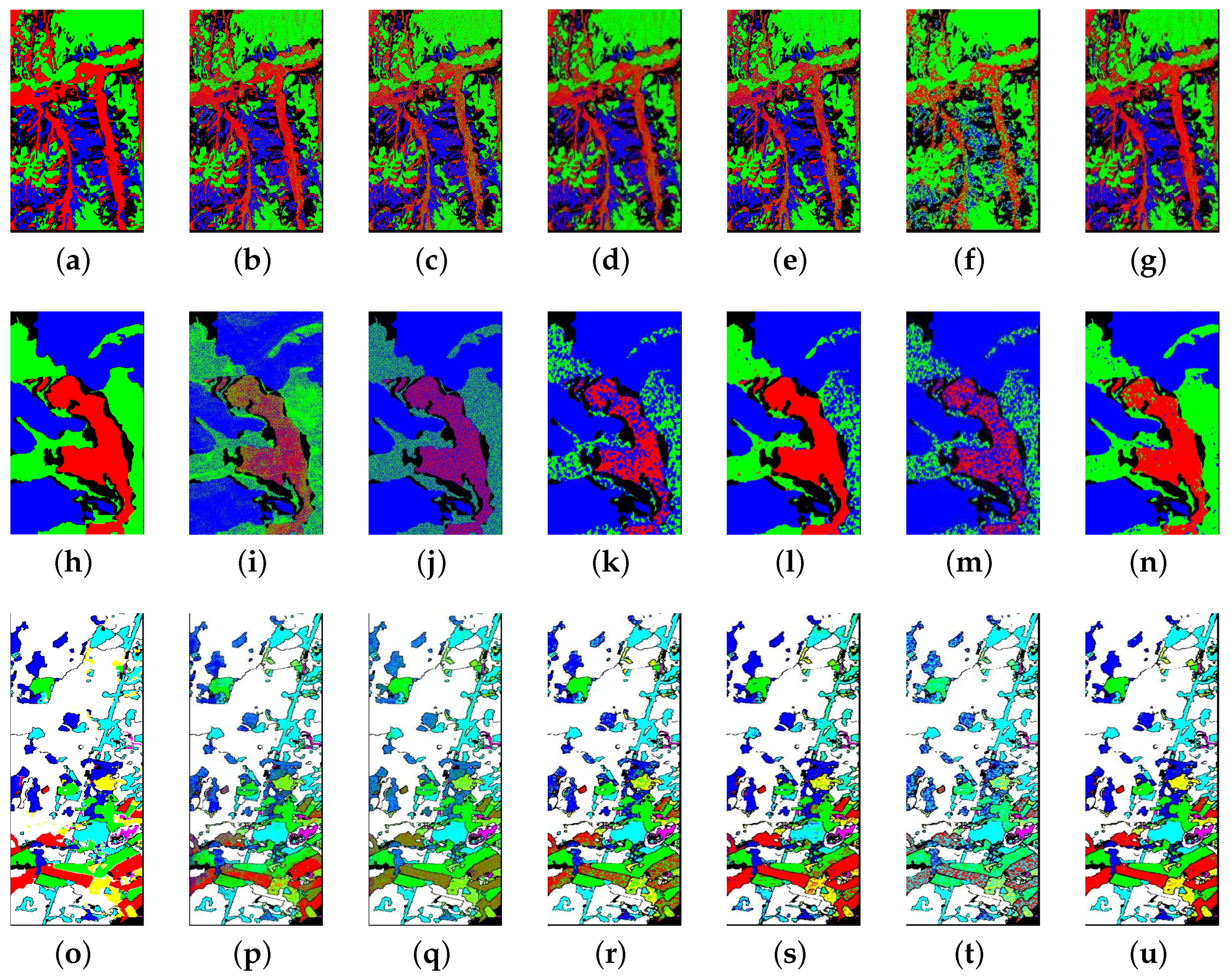
4. Experiments and Discussion
4.1. Data Sets
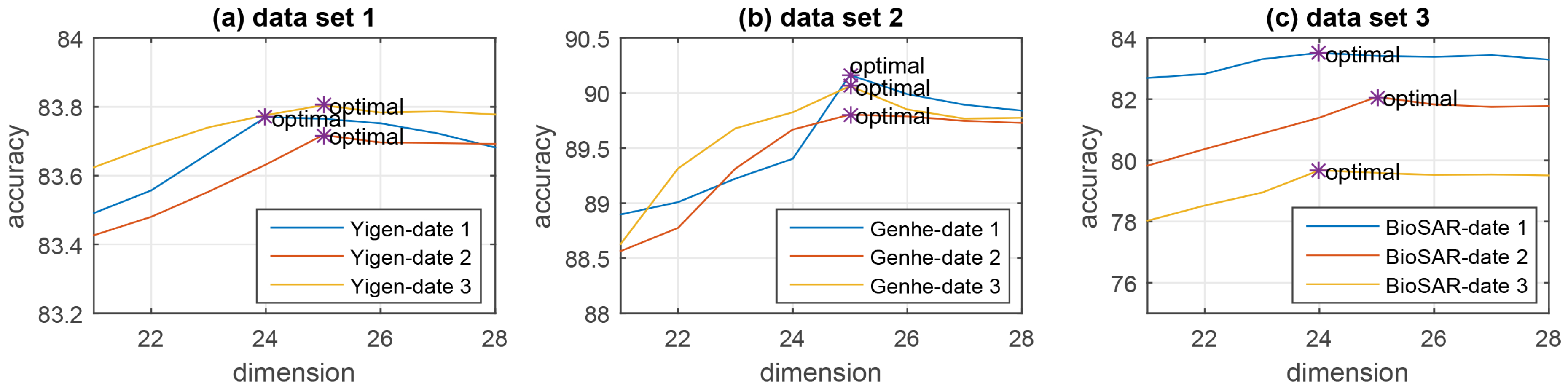
4.1.1. Data Set 1
4.1.2. Data Set 2
4.1.3. Data Set 3
4.2. Experiments and Results Discussion
5. Conclusions
Acknowledgments
Author Contributions
Conflicts of Interest
Abbreviations
| SAR | Synthetic Aperture Radar |
| SVM | Support Vector Machine |
| TD | Target Decomposition |
| MKL | Multiple Kernel Learning |
| PCA | Principle Components Analysis |
| InSAR | Interferometric Synthetic Aperture Radar |
| LLC | Locality-constrained Linear Coding |
| LLE | Locally Linear Embedding |
| PolSAR | Polarimetric Synthetic Aperture Radar |
References
- Jain, A.K.; Duin, R.P.W.; Mao, J. Statistical pattern recognition: A review. IEEE Trans. Pattern Anal. Mach. Intell. 2000, 22, 4–37. [Google Scholar] [CrossRef]
- Richard, H.J. Phenomenological theory of radar targets. Ph.D. Dissertation, Technical University, Delft, The Netherlands, 1970. [Google Scholar]
- Chandrasekhar, S. Radiative Transfer; Clarendon Press: Oxford, UK, 1950. [Google Scholar]
- Robert, C.S.; Eric, P. A review of target decomposition theorems in radar polarimetry. IEEE Trans. Geosci. Remote Sens. 1996, 34, 498–518. [Google Scholar]
- Osmanoglu, B.; Sunar, F.; Wdowinski, S.; Cabral-Cano, E. Time series analysis of InSAR data: Methods and trends. ISPRS J. Photogramm. Remote Sens. 2016, 115, 90–102. [Google Scholar] [CrossRef]
- Zhang, Q.; Wu, Y.; Zhao, W.; Wang, F.; Fan, J.; Li, M. Multiple-Scale Salient-Region Detection of SAR Image Based on Gamma Distribution and Local Intensity Variation. IEEE Geosci. Remote Sens. Lett. 2014, 11, 1370–1374. [Google Scholar] [CrossRef]
- He, C.; Li, S.; Liao, Z.; Liao, M. Texture Classification of PolSAR Data Based on Sparse Coding of Wavelet Polarization Textons. IEEE Trans. Geosci. Remote Sens. 2013, 51, 4576–4590. [Google Scholar] [CrossRef]
- Zhang, L.; Xia, G.S.; Wu, T.; Lin, L.; Tai, X.C. Deep Learning for Remote Sensing Image Understanding. J. Sens. 2015, 501. [Google Scholar] [CrossRef]
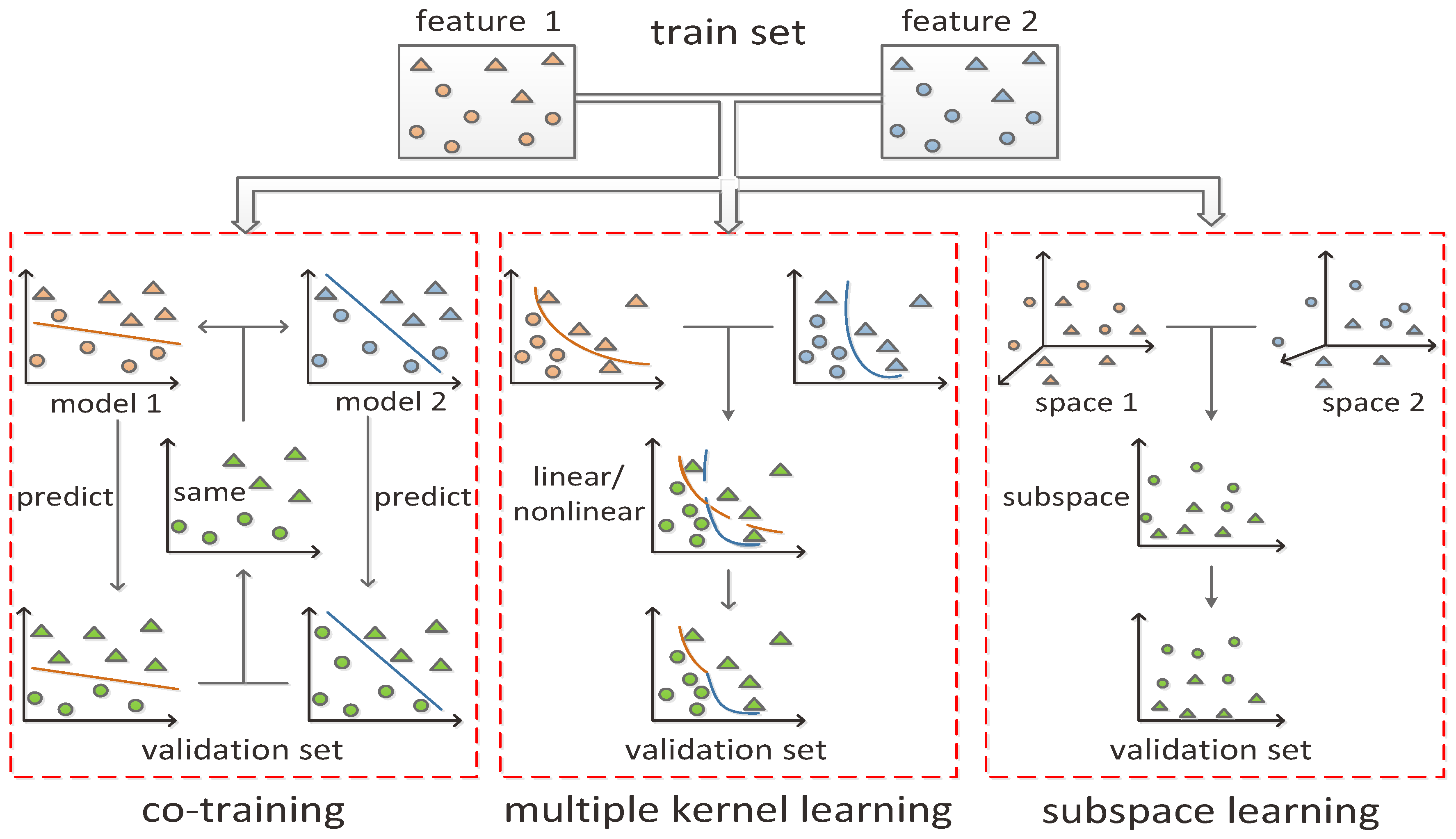
- Xu, C.; Tao, D.; Xu, C. A Survey on Multi-view Learning. Comput. Sci. 2013. [Google Scholar]
- Nigam, K.; Ghani, R. Analyzing the Effectiveness and Applicability of Co-Training. In Proceedings of the Ninth International Conference on Information and Knowledge Management, McLean, VA, USA, 6–11 November 2000; pp. 86–93. [Google Scholar]
- Gonen, M.; Alpaydin, E. Multiple Kernel Learning Algorithms. J. Mach. Learn. Res. 2011, 12, 2211–2268. [Google Scholar]
- Lu, H.; Plataniotis, K.N.; Venetsanopoulos, A. Multilinear Subspace Learning: Dimensionality Reduction of Multidimensional Data; Chapman & Hall/CRC: Boca Raton, FL, USA, 2013. [Google Scholar]
- Blum, A.; Mitchell, T. Combining Labeled and Unlabeled Data with Co-Training. In Proceedings of the Workshop on Computational Learning Theory, COLT, Madison, WI, USA, 24–26 July 1998; Morgan Kaufmann Publishers: Burlington, MA, USA, 1998; pp. 92–100. [Google Scholar]
- Rakotomamonjy, A.; Bach, F.; Canu, S.; Grandvalet, Y. SimpleMKL. J. Mach. Learn. Res. 2008, 9, 2491–2521. [Google Scholar]
- Jolliffe, I. Pincipal Component Analysis, 2nd ed.; Springer Series in Statistics; Springer: New York, NY, USA, 2002. [Google Scholar]
- Estrada, F.J.; Fleet, D.J.; Jepson, A.D. Stochastic Image Denoising. In Proceedings of the British Machine Vision Conference, BMVC 2009, London, UK, 7–10 September 2009. [Google Scholar]
- Wang, J.; Yang, J.; Lv, F.; Huang, T.; Gong, Y. Locality-Constrained Linear Coding for Image Classification. In Proceedings of the IEEE Conference on Computer Vision and Pattern Recognition, San Francisco, CA, USA, 13–18 June 2010; Volume 119, pp. 3360–3367. [Google Scholar]
- Roweis, S.T.; Saul, L.K. Nonlinear Dimensionality Reduction by Locally Linear Embedding. Science 2000, 290, 2323–2326. [Google Scholar] [CrossRef] [PubMed]
- Donoho, D.L. Compressed sensing. IEEE Trans. Inf. Theory 2006, 52, 1289–1306. [Google Scholar] [CrossRef]
- Luis Vergara and Antonio Soriano and Gonzalo Safont and Addisson Salazar. On the fusion of non-independent detectors. Digit. Signal Process. 2016, 50, 24–33. [Google Scholar]


| Type | Coherent Feature | Incoherent Feature | Fusing Feature | |||
|---|---|---|---|---|---|---|
| Co-training | Simple MKL | PCA | Proposed Method | |||
| Accuracy on Data Set 1 | 73.2777 | 65.3550 | 69.4196 | 73.0301 | 64.7154 | 83.7703 |
| 54.0009 | 63.8058 | 70.9354 | 57.9711 | 83.7181 | ||
| 48.0356 | 60.5309 | 71.1018 | 61.2217 | 83.8048 | ||
| Accuracy on Data Set 2 | 57.0702 | 46.5187 | 67.3346 | 83.5341 | 66.2782 | 90.1641 |
| 46.2600 | 66.8268 | 83.7032 | 66.3161 | 89.8039 | ||
| 47.0494 | 73.4284 | 83.4196 | 66.4479 | 90.0633 | ||
| Accuracy on Data Set 3 | 53.8057 | 44.6433 | 71.5634 | 73.6971 | 52.6820 | 83.5168 |
| 33.7141 | 67.1748 | 73.6069 | 61.7849 | 82.0731 | ||
| 47.0471 | 73.8655 | 74.6321 | 59.0582 | 79.6735 | ||
| Type | Coherent Feature | Incoherent Feature | Fusing Feature | |||
|---|---|---|---|---|---|---|
| Co-training | Simple MKL | PCA | Proposed Method | |||
| Time Cost of Data Set 1 (m:s) | 12:46 | 12:13 | 41:23 | 30:35 | 28:26 | 19:17 |
| 13:33 | 43:07 | 26:12 | 27:40 | 18:13 | ||
| 12:29 | 43:18 | 36:04 | 33:37 | 17:34 | ||
| Time Cost of Data Set 2 (m:s) | 11:32 | 11:15 | 39:46 | 26:17 | 22:14 | 15:11 |
| 12:01 | 36:34 | 25:40 | 23:31 | 14:12 | ||
| 11:41 | 43:22 | 24:16 | 25:05 | 13:06 | ||
| Time Cost of Data Set 3 (m:s) | 16:07 | 16:20 | 53:56 | 34:09 | 32:17 | 22:04 |
| 15:41 | 58:26 | 33:50 | 30:11 | 23:07 | ||
| 15:07 | 53:05 | 34:21 | 32:27 | 21:16 | ||
| Data Set 1 | Bare Land (Red) | Forest (Green) | Farmland (Blue) |
| bare land | 91.2493 | 4.1328 | 4.6180 |
| forest | 2.6086 | 96.1337 | 1.2577 |
| farmland | 5.2665 | 3.8476 | 90.8860 |
| Data Set 2 | Building (Red) | Bare Land (Green) | Forest (Blue) |
| building | 87.5113 | 10.3495 | 2.1392 |
| bare land | 0.1025 | 90.3968 | 9.5007 |
| forest | 0.0955 | 2.1107 | 97.7938 |
| Data Set 3 | Farmland (Red) | Pine Trees (Green) | Spruces (Yellow) | Birches (Cyan) | Grassland (Blue) |
|---|---|---|---|---|---|
| farmland | 97.6495 | 1.9156 | 0.2967 | 0.0153 | 0.1228 |
| pine trees | 0.6353 | 98.8160 | 0.1959 | 0.0041 | 0.3486 |
| spruces | 0.2482 | 0.3911 | 97.3556 | 0.0134 | 1.9916 |
| birches | 1.5294 | 6.8386 | 0.1051 | 87.2796 | 4.2473 |
| grassland | 0.0099 | 0.1972 | 0.0657 | 0.0017 | 99.7117 |
© 2017 by the authors. Licensee MDPI, Basel, Switzerland. This article is an open access article distributed under the terms and conditions of the Creative Commons Attribution (CC BY) license (http://creativecommons.org/licenses/by/4.0/).
Share and Cite
He, C.; Han, G.; Feng, D.; Du, J.; Liao, M. A Sparse Manifold Classification Method Based on a Multi-Dimensional Descriptive Primitive of Polarimetric SAR Image Time Series. ISPRS Int. J. Geo-Inf. 2017, 6, 97. https://doi.org/10.3390/ijgi6040097
He C, Han G, Feng D, Du J, Liao M. A Sparse Manifold Classification Method Based on a Multi-Dimensional Descriptive Primitive of Polarimetric SAR Image Time Series. ISPRS International Journal of Geo-Information. 2017; 6(4):97. https://doi.org/10.3390/ijgi6040097
Chicago/Turabian StyleHe, Chu, Gong Han, Di Feng, Juan Du, and Mingsheng Liao. 2017. "A Sparse Manifold Classification Method Based on a Multi-Dimensional Descriptive Primitive of Polarimetric SAR Image Time Series" ISPRS International Journal of Geo-Information 6, no. 4: 97. https://doi.org/10.3390/ijgi6040097