Impact of High-Resolution Topographic Mapping on Beach Morphological Analyses Based on Terrestrial LiDAR and Object-Oriented Beach Evolution

Abstract

This research applied terrestrial LiDAR for laboratory beach evolution experiments to quantify the impact of resolution on topographic mapping and change analyses. The multi-site registration and multi-temporal scanning processes produced high accuracy (−0.002 ± 0.003 m) topographic models in a wave tank environment. Morphological analyses based on surface change and profiles showed that models of all resolutions were capable of capturing major sediment changes in relatively smooth areas. However, higher resolution models were necessary in areas with rough surfaces and sudden elevation changes, while coarser resolution models smoothed the roughness and underestimated feature height (e.g., peaks and troughs). Decreasing resolutions from 1 to 10 cm resulted in a 2% underestimation of erosional volumes with a linear regression of y = −0.0964x + 0.4185 (R² = 0.9651) and 3.5% overestimation of depositional volumes with a linear regression of y = 0.0664x + 0.3308 (R² = 0.3645). However, its impact on erosion and deposition volume assessment based on object-oriented beach evolution analysis is less significant, except when fragment objects dominate the sediment changes. For Coastal Morphology Analyst (CMA), the impact of resolution is more observable through 2D object mapping in terms of object size, number, and spatial distribution. Finally, wave modeling experiments proved that resolutions caused significant changes on the behavior of the maximum wave height, the shape of the wave fronts and magnitudes of the currents.

1. Introduction

Topographic mapping is an important subject in riverine, estuarine and coastal environments, related to a wide range of issues such as land loss, bank erosion, wetland degradation, barrier island protection, and wildlife conservation [1,2]. In areas with low gradient topography like coastal wetlands, small elevation changes in a few centimeters can sometimes cause flood in some areas, significantly alter salinity, and hence transform the distribution of vegetation species [3,4]. As an ancillary data resource, topographic models can be further fused with other data to assist classifications of land cover/use types, vegetation species, mineral types, wildlife habitats, and estimation of carbon stocks [4,5]. All these important applications rely heavily on accurate topographic mapping.

Methods for monitoring sediment topographic changes include measurement of elevation profiles, video imagery, and laser profiling. Cross section elevation profiling at discrete sample locations is a method commonly used in both wave tank experiments and in the field [6,7,8]. Coops, Geilen, Verheij, Boeters and van der Velde [6] used recording poles to determine elevation profiles and volume change in an outdoor wave tank experiment, a simple yet effective method to monitor sediment variations and estimate the volume of erosion and/or deposition. However, considering the spatial heterogeneity of beaches, analysis based on a limited number of profiles may be insufficient for accurate calculation of morphological changes over the entire area [9] and may overlook areas with severe sediment change due to the need to predetermine profile locations for periodical surveys and the difficulty in predicting locations of severely eroded areas. Higher accuracy often requires a larger array of sensors or more measurements [10], which can be challenging and costly in both laboratory and field environments using these discrete measurement methods. Therefore, methods with non-intrusive and continuous surface mapping are preferred for many applications.

As a non-intrusive method, video imagery has been used in many experiments for sediment erosion and deposition analysis [11,12,13], dune evolution [14], wave morphology [10,15], and swash flow [16]. One application of video imagery is two-dimensional profile analysis and classification. Foote and Horn [15] and Erikson and Hanson ([10]) used video imagery to measure wave and sediment morphological dynamics using cameras mounted on tripods placed along the side of a glass tank. For 3D morphological mapping, Palmsten and Holman ([9]) used video imagery to construct high-resolution (10 cm) morphological models and extracted 16 elevation profiles every 15 min for 20 h. The results showed an average root-mean-square error (RMSE) of 0.05 m with a range between 0.03 to 0.08 m in reference to the manual measurements. Stationary video imagery and stereo photogrammetric mapping has demonstrated advantages including non-intrusive survey [9], high-spatial and multi-temporal resolution mapping [10], 3D morphological modeling and volume estimation [9]. However, it has limitations in large-area mapping due to the need of significantly increased station numbers and the short distance requirement between stations for acquiring stereo images. Also, the complicated processes necessary for dealing with image distortion and rectification can be challenging to some users [9]. Mounting the cameras on UAV (unmanned aerial vehicle) can expand their usefulness in large-area field surveys [17].

Known as a high-precision and high-resolution mapping tool, terrestrial LiDAR has become more reliable, accessible and popular in various field applications [18,19,20]. The LiDAR sensors can be mounted on aircraft, UAV, mobile vehicles, and stationary tripods [18,21]. A LiDAR sensor mounted on a tripod is called a terrestrial LiDAR system or terrestrial laser scanner and is suitable for in situ data collection in both laboratory and field environments. Terrestrial LiDAR requires much simpler post processing than photogrammetric stereo mapping methods and has no need for distortion correction yet produces high point density and highly accurate measurements. This type of laser survey is non-intrusive to the sediment surface and produces color-coded data with accurate three-dimensional coordinates with intensity information. These natural color (RGB) 3D coordinates and intensity information are applicable to differentiate sediment types, vegetation cover, soil moisture and surface roughness [18,20,21,22].

In recent years, terrestrial LiDAR and UAV have demonstrated great advantages for quick, accurate, and dense 3D topographic mapping and are more commonly used as in situ high-resolution mapping tools to integrate with other field data for interdisciplinary studies. However, the availability of topographic models with different resolutions and their impacts on physical process modeling and topographic change analysis have not been fully explored. Especially, terrestrial LiDAR has not been used for object oriented beach evolution analysis in a wave tank environment, and resolution impact has not been assessed for CMA method. In addition, although different topographic models have been used for wave modeling on various scales, the impact of resolution on wave modeling has not been discussed [23,24]. Moreover, with increasing popularity of high-resolution mapping based on terrestrial LiDAR and UAV, many users face a practical question regarding the choice of resolution to interpolate various topographic products. A common procedure is to determine resolution based on the average point density. However, problems arise when the point density is uneven or gaps with no points exist due to limited laser light penetration in dense vegetation and block of light from limited viewpoints. UAV users encounter similar gaps due to areas with low contrast, smooth texture, or wind impact on tall vegetation. With the presents of gaps, users may adjust to larger resolution values and will need to know the impact of resolution changes on topographic products and applications.

This research aims to quantify the effect of resolution on various topographic mapping, sediment change analysis, wave-induced beach change and beach evolution using terrestrial LiDAR data from wave tank experiments. The experiments discussed below examine the use of different resolutions for morphological feature mapping, 3D and profile-based sediment change analyses, volume assessments, wave modeling, and object-based beach evolution analysis.

2. Methods

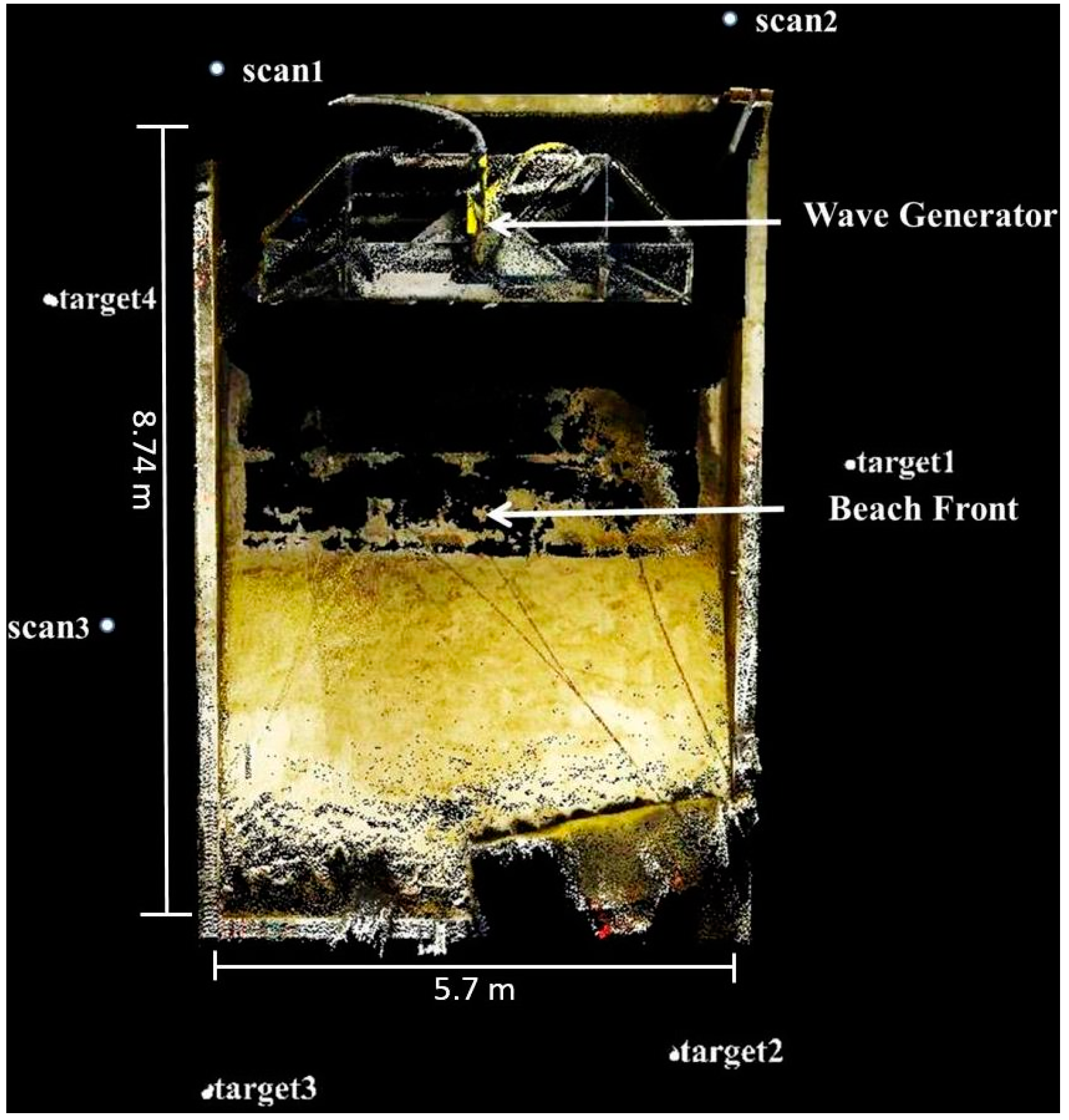
2.1. Laboratory Experiment Setup and Data Collection

The experiment was conducted in an indoor wave tank at Louisiana State University as illustrated in Figure 1. This wave tank is 8.74 m long, 5.7 m wide, and 0.30 m deep and equipped with a wave generator with a LDT (Linear Displacement Transducer) position-sensing system made by MTS Systems Corporation. The distance from the front surface of the wave maker to the end of the wave tank is 6.83 m. The sand is well sorted with a sorting coefficient of 0.48 and has a slight coarse skew with a skewness value of 0.11. The sand has a mean grain size of 0.34 mm and density of 2.65 g/cm³. Figure 2 illustrates the initial beach created at the end of the wave tank with a slope of 15° and five beach profiles with an approximate cross-profile distance of 0.93 m for elevation change analysis. The distance from the beach front to the wave maker front is approximately 3 m. To use these laboratories generated waves to demonstrate the application of terrestrial LiDAR for sediment change mapping, the wave generator was programmed to produce continuous waves with a 0.499 Hz (2 s period) sine waves for three 10-min applications and used terrestrial LiDAR to map the beach morphology before and after each wave application. Three pressure sensors for wave height measurement were evenly placed around 1.7 m in front of the wave maker front, and the measured wave height is 0.06 m.

2.2. High-Resolution Topographical Mapping Based on Terrestrial LiDAR and Wave Tank Experiment

The system used in this research was a Riegl VZ-1000 V-Line 3D Terrestrial Laser Scanner using near infrared wavelength with a range measurement precision of 5 mm and an accuracy of 8 mm for a 100 m range. The Riegl VZ-1000 produces high density mapping with a high rate of sampling: 29,000 to 122,000 measurements/second and is capable of long-range coverage of up to 1400 m. With a horizontal scanning angle of 360° and a vertical scanning angle of 100° (+60° to −40°), the system can produce a 3D panoramic scan of surrounding environments. In addition to the color-coded data with 3D coordinates, each point contains additional intensity information that reflects the strength of wavelength returns from different objects, information that is often used to classify landscape types. When applied in indoor laboratory environments, it can map sediment morphology from multiple positions. The instrument produces 3D color-coded data with high point density and intensity values. These data can be used to reconstruct high-resolution topographic models.

One important analysis of beach dynamics is the change of sand in the swash zone [10]. The swash zone is an area where water waves cover sandbed periodically and where significant sediment erosion and deposition occur [14]. For wave modeling and beach change analysis, it is important to obtain the severely changed swash zone. However, water has a high absorption rate of the near-infrared wavelength used in this LiDAR system. Therefore, this research used wave tank experiment to simulate three periods of wave applications and mapped full beach morphology through the following design. After each wave application, the beach topography is measured at still water, and the water is then slowly drained from the tank, after which another beach topography mapping is done. The tank is slowly refilled with water and the experiment is repeated.

The terrestrial LiDAR system scanned the beach with a 0.002° resolution and a scanning range of 500 m (the minimum scanning distance with a setting of 300 kHz laser pulse repetition rate and 122,000 measurements/second). To capture the entire beach, this experiment conducted multi-site scans at two locations near the end of the wave tank for each survey and added a third location at the side of the beach during the last survey to capture a deeply eroded area that might have been blocked from the other two locations. Four highly reflective cylindrical targets provided by the LiDAR system were evenly distributed around the tank (Figure 1) before and after each 10-min wave application to ensure consistent registration from multi-site and multi-temporal scanning. The LiDAR operation system RiSCAN PRO software used a multi-site registration function and the four targets to accurately register all data from 17 panorama scans through one time of registration process. As a result, a total of four topographic models acquired under no water condition were used in the following beach analysis. Noises from images of nearby walls, frames and beaches reflected by the residual water and with elevations below the wave tank floor were manually removed during the preprocessing stage.

2.3. Wave Modeling Based on High-Resolution Morphological Models

Two different numerical models have been applied in order to reproduce the wave and currents induced by waves with different resolution topographic models: The WAPO [25] and COCO models [24] that have been successfully used and validated in previous studies as described in Silva, Baquerizo, Losada and Mendoza [24]. The numerical model set up has a grid size of 551 × 431 and a friction coefficient of 0.001 with open boundary conditions. The experiment is an off-line coupling. Using the velocity potential (output of WAPO), the instantaneous free surface elevation and the velocities are calculated. With these parameters the components of the radiation stress tensor are evaluated (The radiation stress tensor is the input for the COCO). The wave propagation WAPO model solves a second-order approximation of the modified version of the mild-slope, which is capable of representing open, partially reflected and fully transmitting conditions for both incoming and outgoing waves was developed. This linear WAPO can solve implicitly refraction, reflection, and diffraction. The model is robust and can be used in complex geometries and has fewer restrictions associated with wave obliqueness at boundaries than traditional models based on the mild-slope equation. Using the output of WAPO model, radiation stresses and wave driven currents are calculated by means of the COCO model.

2.4. Analysis of Resolution Impact on Beach Topographic Mapping and Beach Evolution Analysis

The goal of this section is to use the high-density beach data derived from terrestrial LiDAR to evaluate and quantify the impact of resolution choices on common topographic analyses. Considering the fact that terrestrial LiDAR and UAV are often used for high-resolution mapping within 10 cm [26,27], this research generated a set of topographic models ranging from 1 cm to 10 cm resolution at 1 cm increments for the following analyses through a resampling processing by overlaying a grid on top of the point clouds and assigning the minimum elevation to the elevation value of a cell.

The total volume of eroded and/or deposited sediment can be calculated from the elevation-change map. This research used the initial and last beach topographies at 10 different resolutions in calculating the amount of volume changes as a result of erosion and deposition thereby assessing the effect of the increasing of resolution. To examine the impact of different resolutions on beach profile analysis, this research analyzed the five beach elevation profiles as illustrated in Figure 2 based on the last beach model with resolutions of 1, 5, and 10 cm. The beach profiles from the initial beach model with 1 cm resolution were added as a reference for sediment changes. Additionally, this research used the four 1-cm resolution and multi-temporal beach models to illustrate the usefulness of high-resolution models for profile-based beach evolution analysis especially for morphological features with smaller sizes.

2.5. Application of an Object-Based CMA Method for Beach Evolution Analysis Based on High-Resolution Beach Models

Beach evolution analysis examines the gradual sediment changes over time. When 3D topographic models are available, users often use a pixel-based elevation change map for sediment change analysis. In recent years, a simple effective object-oriented tool, Coastal Morphology Analyst (CMA), has been developed for coastal morphological change analysis by Liu et al. [28]. This tool provides a way to examine sediment change patterns and has a great potential in applications such as beach nourishment.

Given two topographic models, the elevation change is represented by subtracting an earlier model from the next in the time sequence. Based on a predefined threshold of elevation change value, each pixel is then classified as erosional, depositional, or area of no significant change. Users can define this threshold based on their need or preferences in certain applications. The remaining pixels with elevation change within the threshold are classified as areas with no significant change. Based on maps of these elevation changes and classified labels, the CMA method then forms object boundaries by grouping neighboring pixels with the same erosional or depositional labels. In order to eliminate salt-and-pepper noises from small and random pixels, CMA applies the minimum pixel number of an object to determine the minimal object size.

3. Results

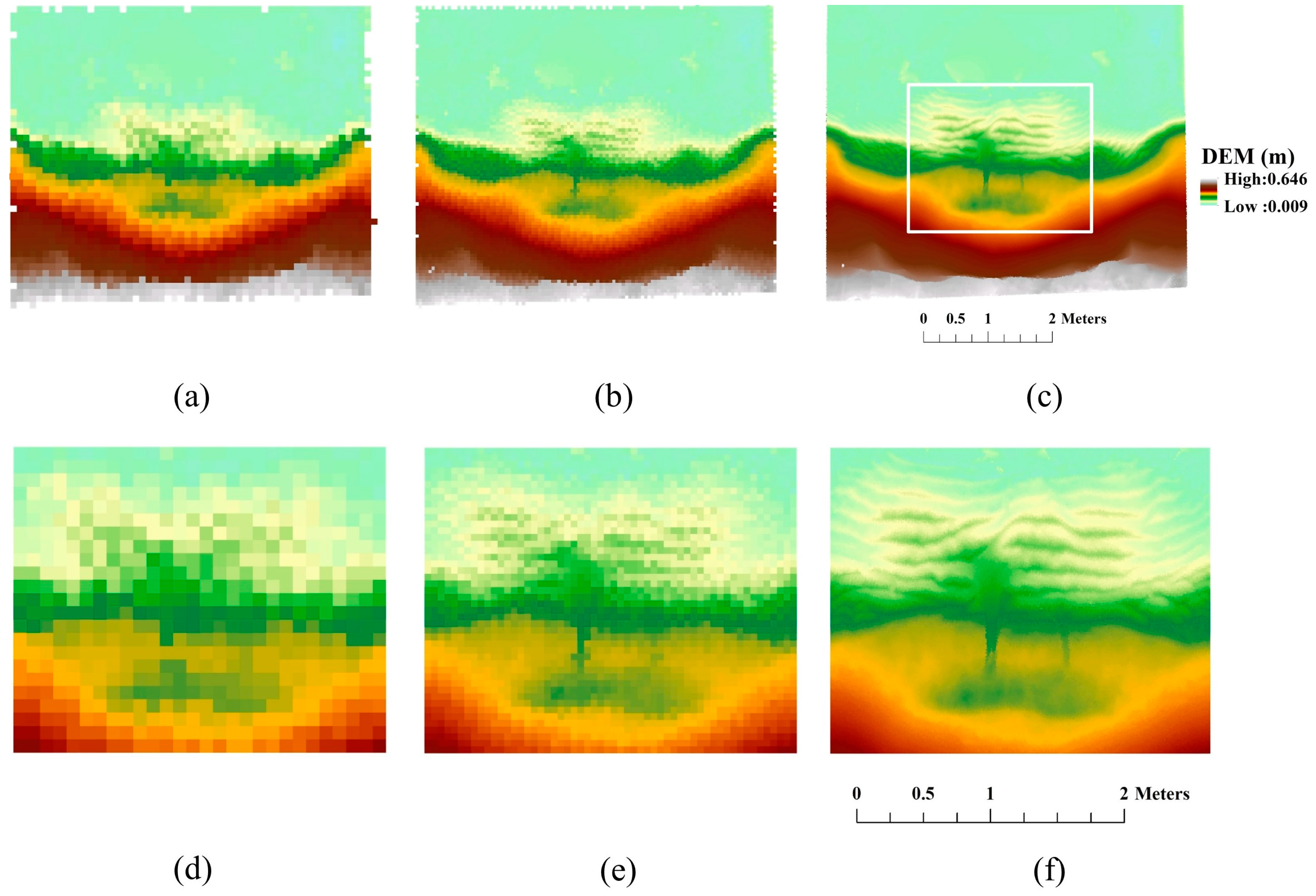
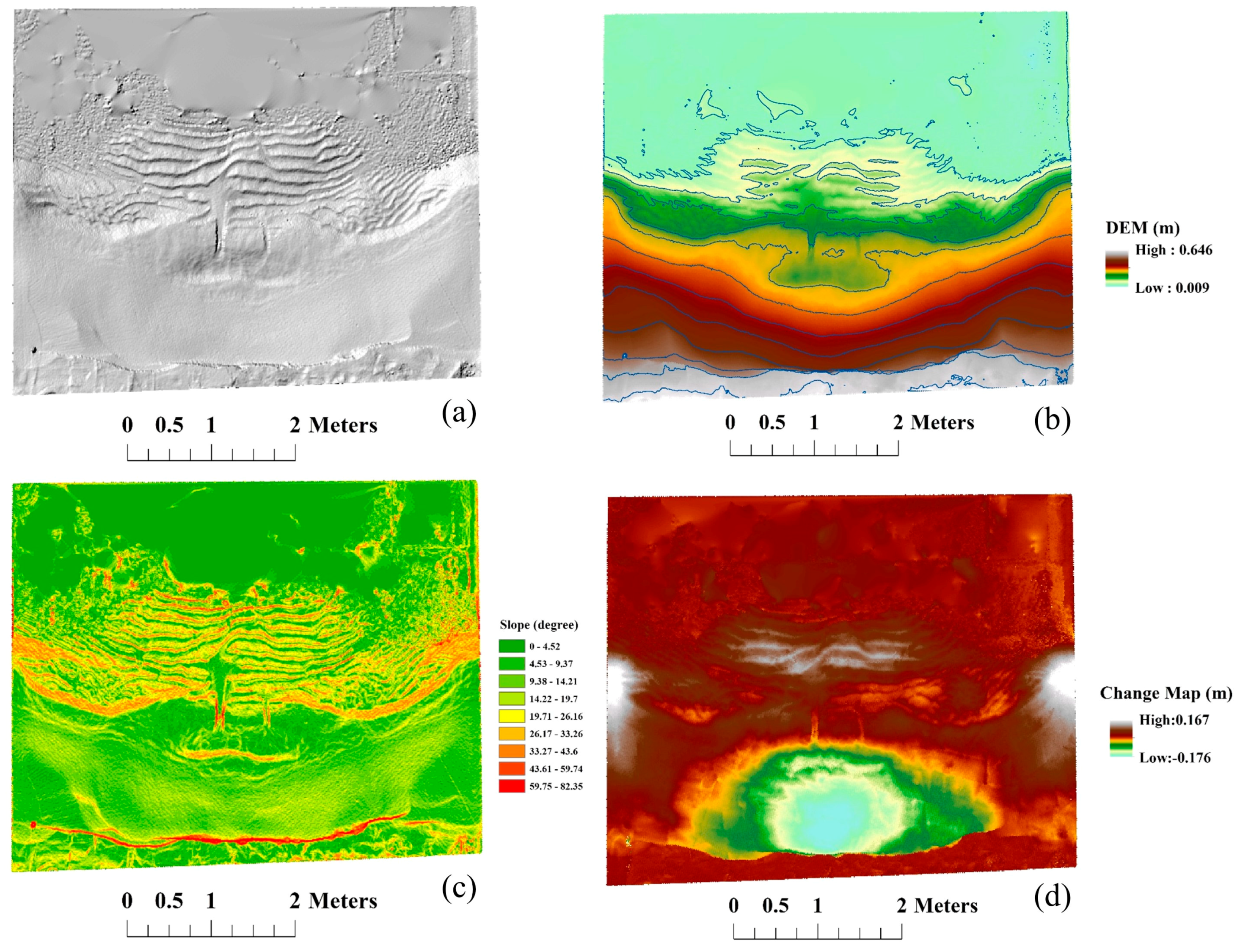
3.1. High-Resolution Laboratory Beach Topographic Mapping Based on Terrestrial LiDAR

The LiDAR survey data for the four beach statuses without water were used for the following analysis. The derived data have an average point density of 4 points/cm² for two scan positions and 11 points/cm² for three scan positions. The data for each beach mapping were then resampled into beach models through minimum values. The registration process produced a standard deviation of 0.009 m. To assess the potential errors introduced by the multi-site and multi-temporal scanning and registration process, this experiment used thirty randomly distributed points in the undisturbed beach at the end of the wave tank based on the first and last beach models with 1 cm resolution. The results showed an accuracy of −0.002 ± 0.003 m, indicating no significant errors introduced.

To examine the impact of resolutions on beach topographic analysis and applications, the same resampling method was used to resample the data with resolutions from 1 to 10 cm. Figure 3 demonstrates the high-resolution (1 cm) topographic products including topographic model, slope map, aspect, and hill-shaded relief map. Figure 3a shows the hill-shaded relief map of the laboratory beach morphology with an enhanced 3D perception, which is especially useful for the analysis of low-relief areas such as ripple patterns. Figure 3b shows a contour map with 5-cm intervals overlaid on top of the 1 cm resolution topographic model. Comparing to the hill-shaded relief map, the contour map generalizes the topography into a few zones of equal elevation ranges and provides effective assistance in recognizing elevation trends and patterns. The slope map in Figure 3c highlights areas with steep slopes in red; this can be used as a tool to enhance ripple patterns as well as to locate areas of significant sediment erosion. Figure 3d is the commonly used elevation change map.

Overall, Figure 3 showed that Sediment in the middle and upper areas of the swash zone was washed downslope and deposited at the beach front. The most significant sediment erosion occurred at the middle area of the beach, forming a pond. In addition, these results demonstrate the advantage of high-resolution mapping to detect morphological features with smaller sizes. The smallest morphological feature detected in this 1 cm resolution model is the 3 cm wide ripples at the beach front. The ripples on the floor were mainly distributed at the center half of the tank due to the proximity to the most severely eroded upper areas and the interference of side walls with water waves. The pixel-based map of elevation changes in Figure 3d shows that the elevation changes range from −0.176 m to 0.167 m. The most significantly eroded area locates at the center at the back of the beach with gradual decline to both sides. The most significantly deposited areas include the lower elevation area right next to the significantly eroded area and the areas next to the walls on both sides. For the impact of resolution on topographic feature mapping, all three beach topographic models with different resolutions (1 cm, 5 cm, and 10 cm) in Figure 4 detect similar major erosional and depositional areas and patterns. The erosion contour demonstrated a nearly symmetrical pattern from the center line at L3 (Figure 2) with gradual decay approaching the walls of the wave tank. However, with the improvement of resolution, beach models with higher resolutions can capture more detailed morphological features. For example, the thin layers of sediment deposit with ripple patterns seen at the front center are well captured by the topographic model with 1 cm and 5 cm resolutions but are obscure in the 10 cm resolution model. Similarly, the smaller ripple patterns following the edge of beach front were well captured in the 1 cm model but not recognizable in the 5 cm model. These small scale features are useful for certain applications as indicators for dominant water flow directions or prevailing wind directions.

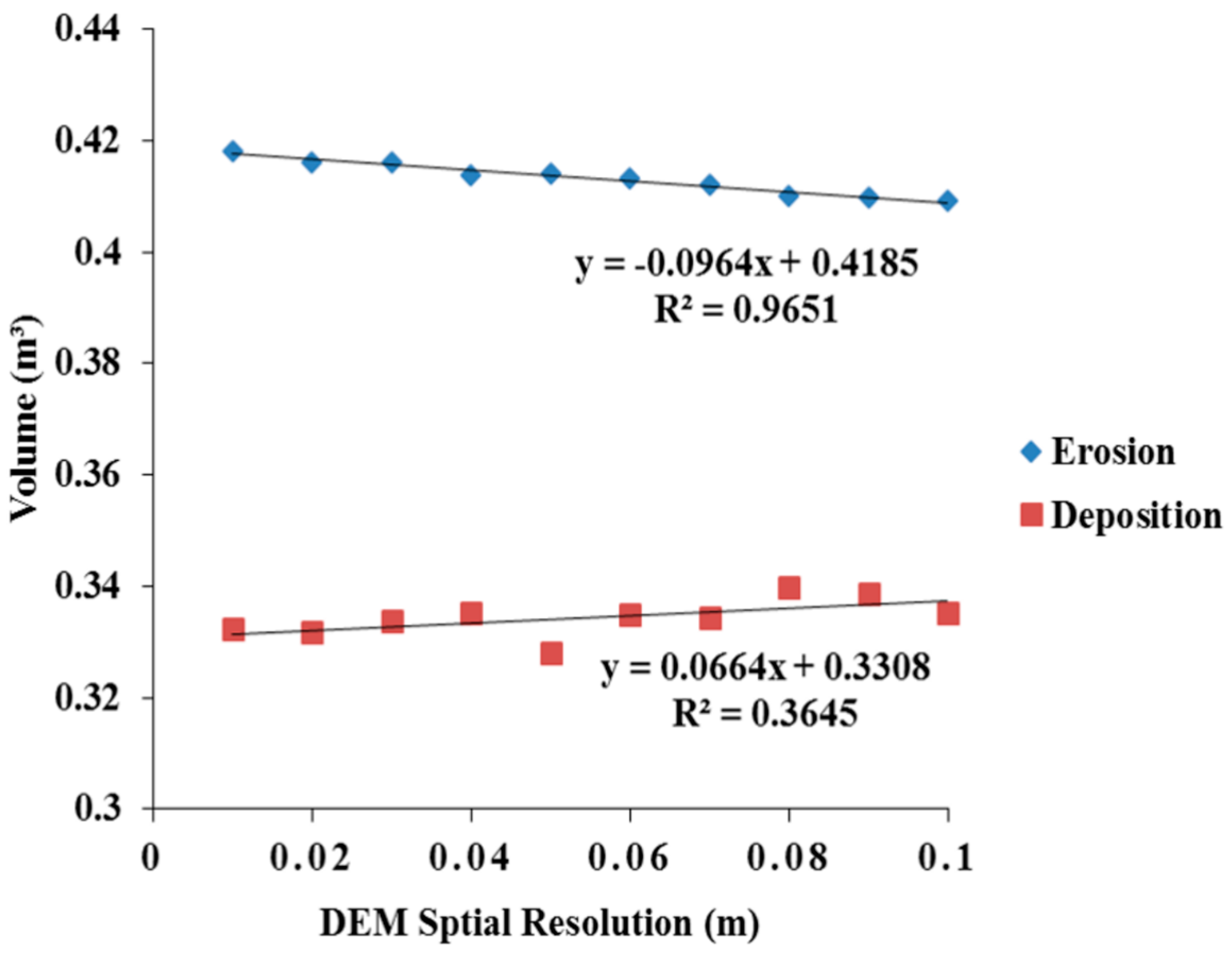
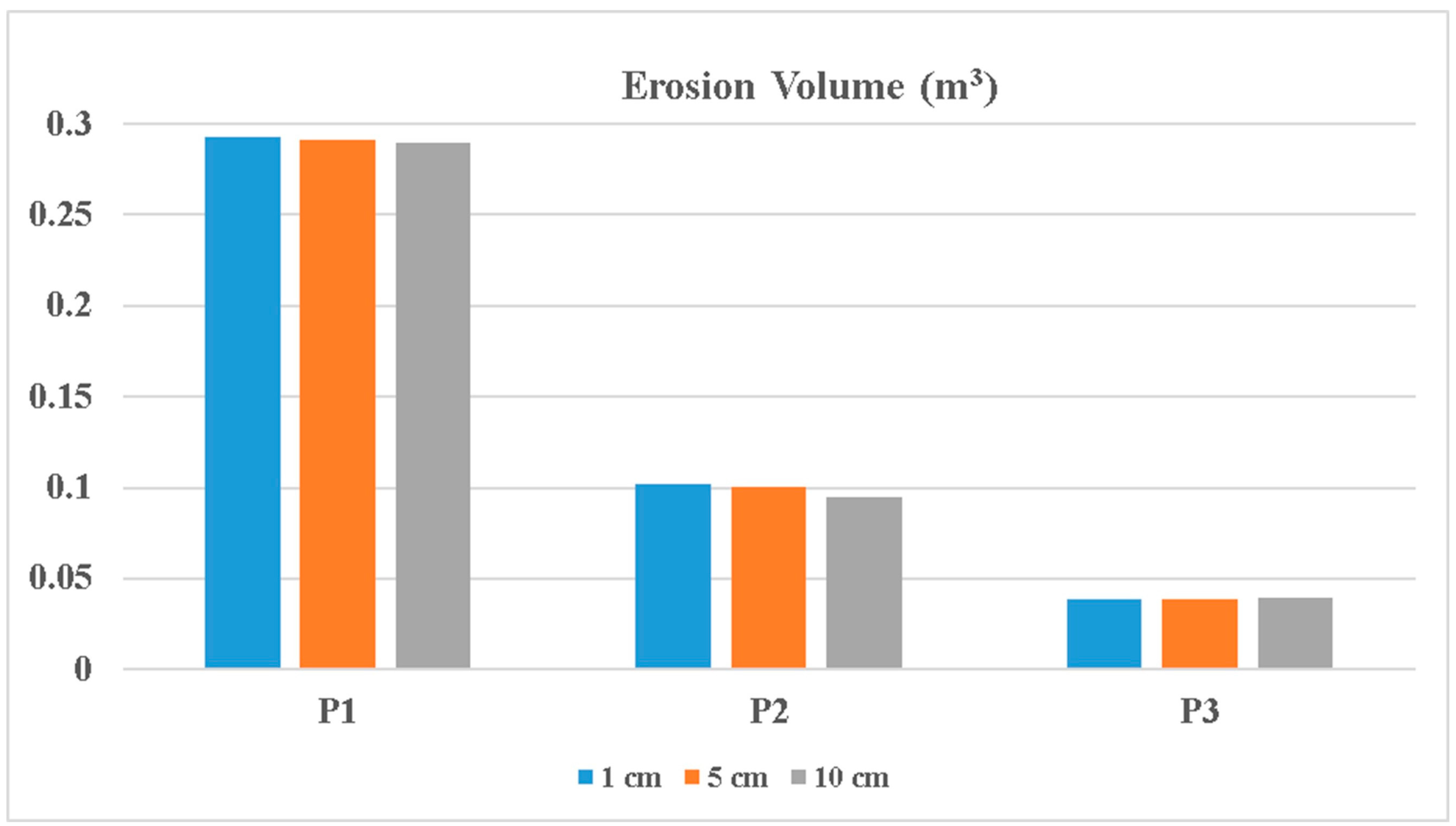
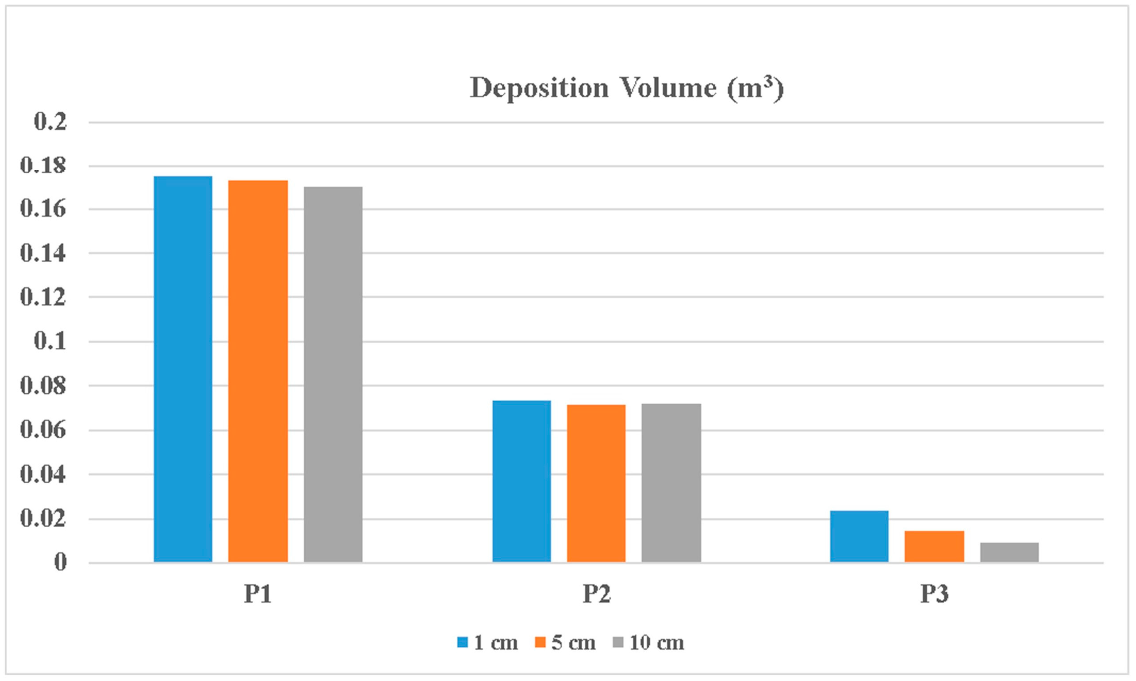
3.2. Impact of Resolution on Volume Change Assessment

The changes in beach volume between the initial and final beach models of the entire study site were calculated. Pixels with negative values were classified as erosional areas while pixels with positive values were classified as depositional areas. Depositional volume, erosional volume, and net change were extracted from models with resolutions ranging at 1 cm increments from 1 cm to 10 cm. Figure 5 summarizes the relationship between spatial resolutions and derived erosional and depositional areas. As the spatial resolution changed from 1 cm to 10 cm, erosional volume decreased from 0.41799 m³ to 0.40925 m³ with a total underestimation of 2%. There is a strong linear regression of y = −0.0964x + 0.4185 with an R² of 0.9651. With the increase of cell size, depositional volume increased from 0.32815 m³ to 0.33986 m³ with a total overestimation of 3.5%. There is a linear regression of y = 0.0664x + 0.3308 with an R² of 0.3645. Overall, the results indicated that interpolating morphological models with coarser resolutions leads to underestimations of erosional volume and overestimation of depositional volume.

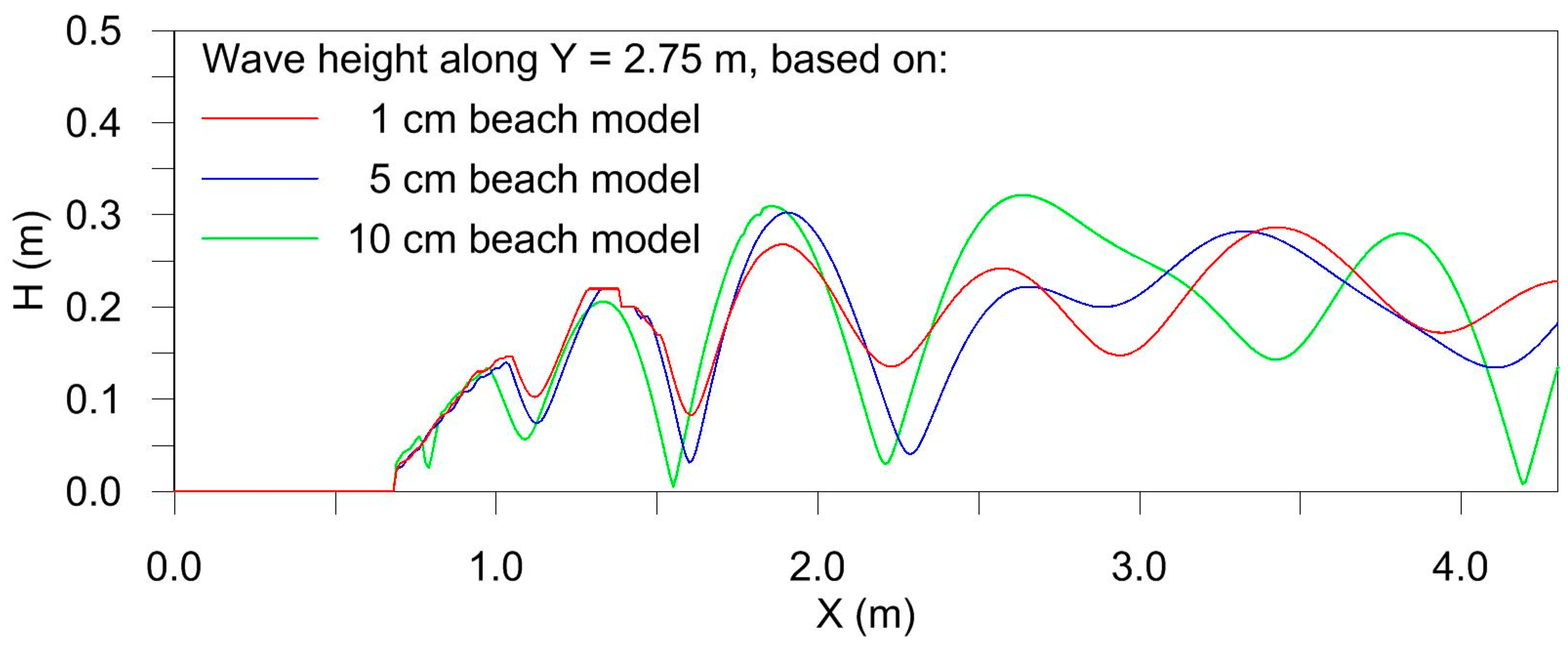
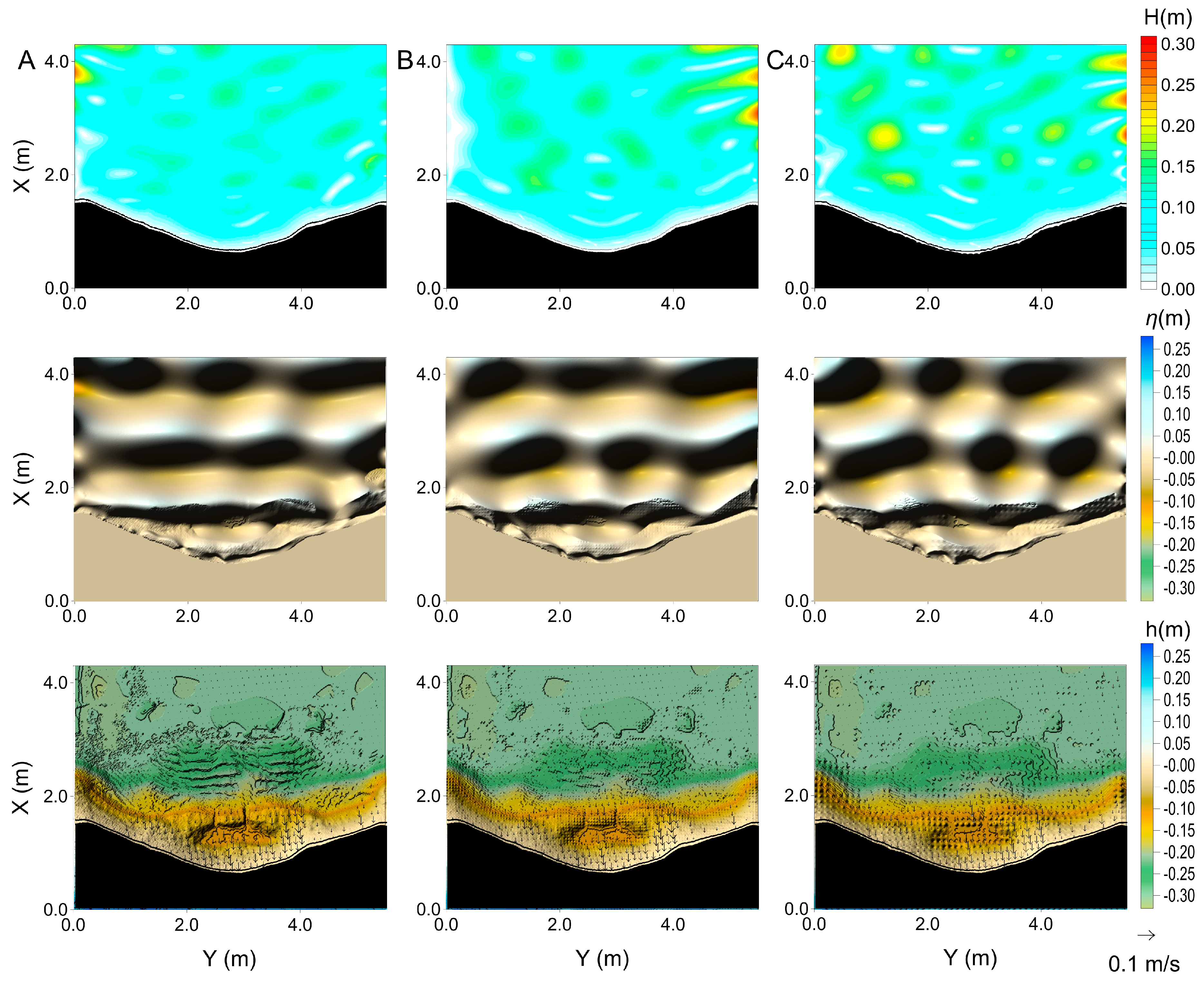
3.3. Wave Modeling Based on High-Resolution Topographic Models

Three different beach models were used employing the data collected, with a spatial resolution of 1, 5 and 10 cm, called A, B and C, respectively. Figure 6 shows the results obtained with the beach models A, B and C, left to right. The same figure shows, from the top to the bottom, the local wave height, the instantaneous free surface and the wave induced currents superimposed on the beach models employed. When all the cases were run with the same conditions except beach models with different resolutions, there is substantial dependence on the hydrodynamic results obtained, phase and magnitude of the wave height and wave driven currents. All cases showed that as the wave propagates from landward, the wave height increases in the central part of the shore and decreases in the lateral sections, where the wave front delays, and a current pattern is generated, modifying the forcing mechanisms of the current velocity field and the bed contours. However, there are significant changes in the behavior of the maximum wave height, the shape of the wave fronts and magnitudes of the currents. Figure 7 plots the wave height profiles along the longitudinal Y = 2.75 m for the modeling results derived based on (a) 1 cm, (b) 5 cm and (c) 10 cm beach models. The relative difference between (a) and (b) and (a) and (c) are 16% and 36%, respectively. These results illustrate the importance of the quality of the topographic data for the hydrodynamic evaluation and their potential consequences in topographic modeling.

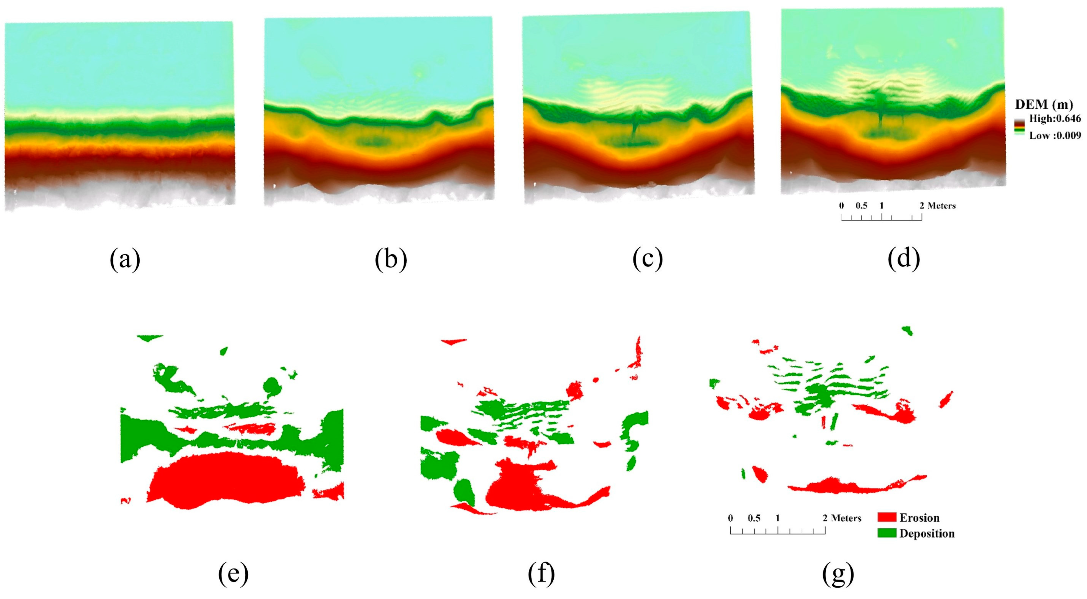
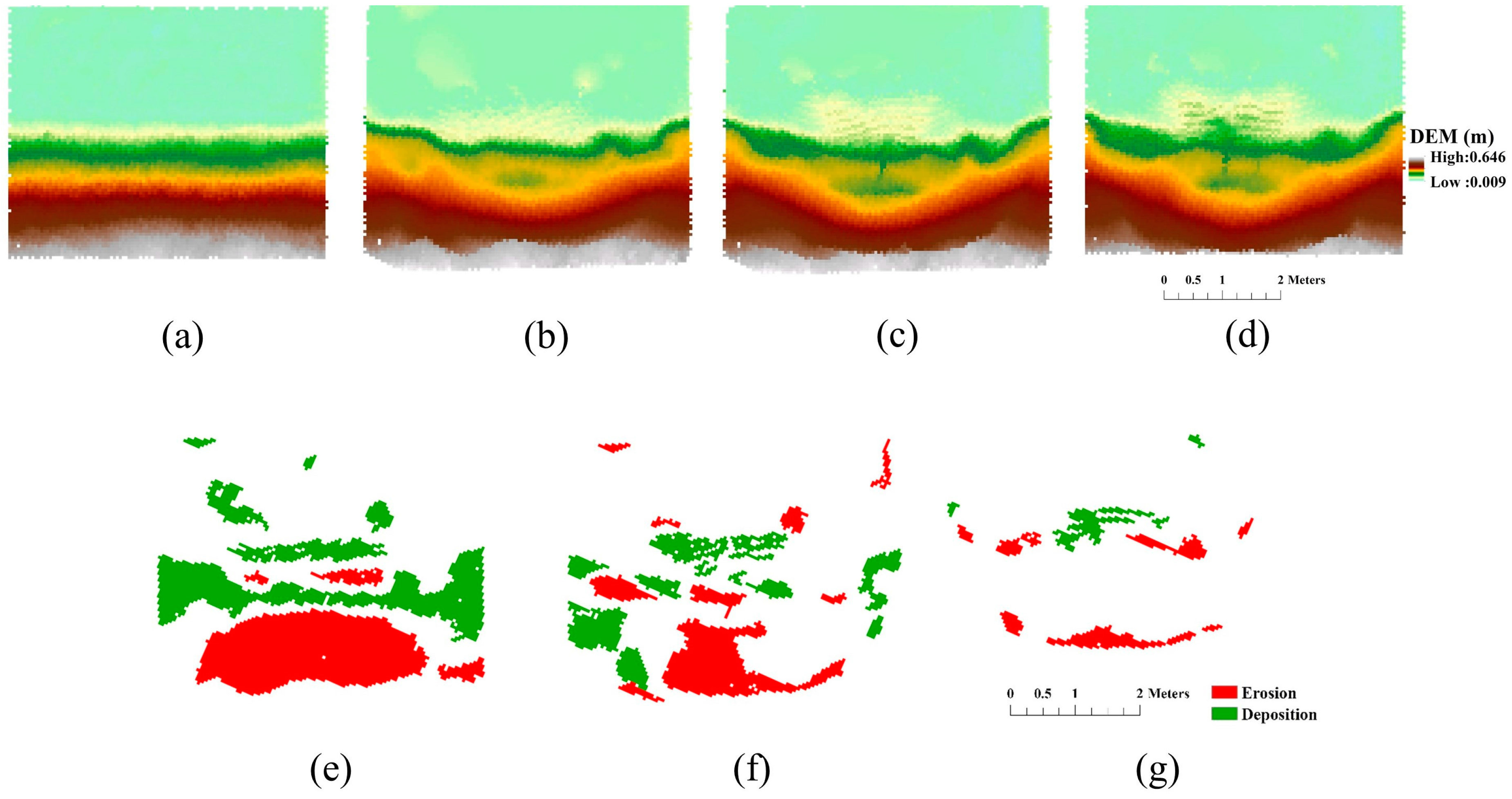
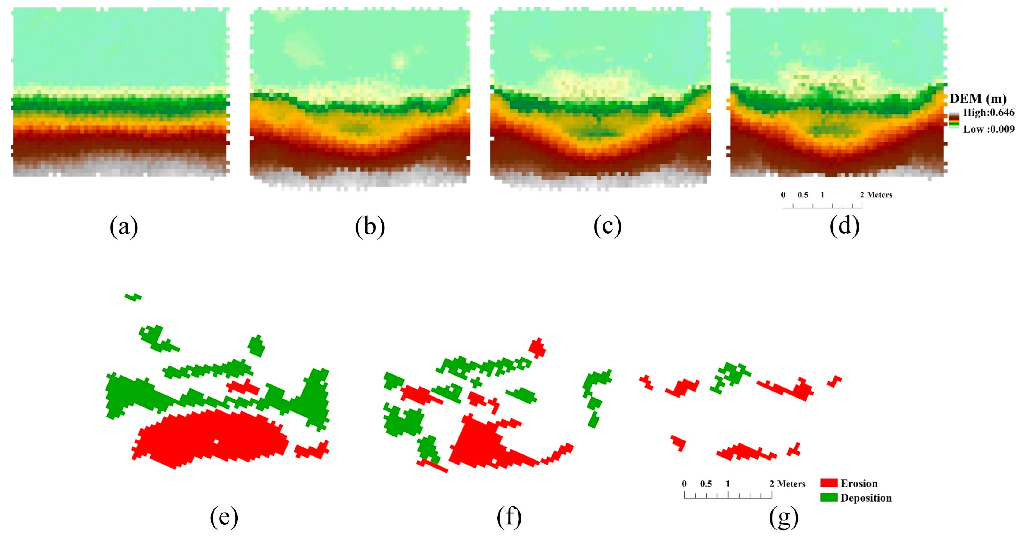
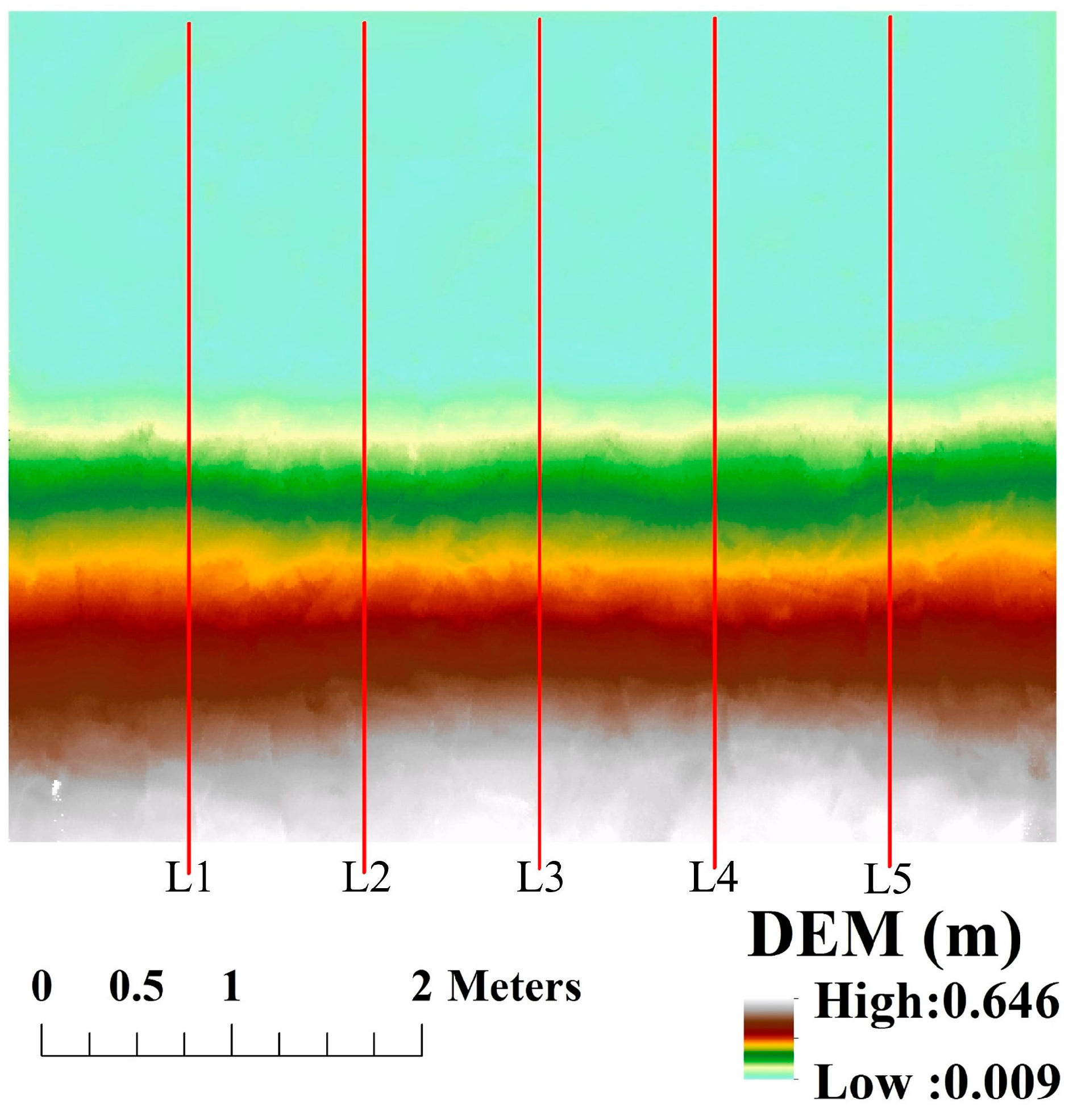
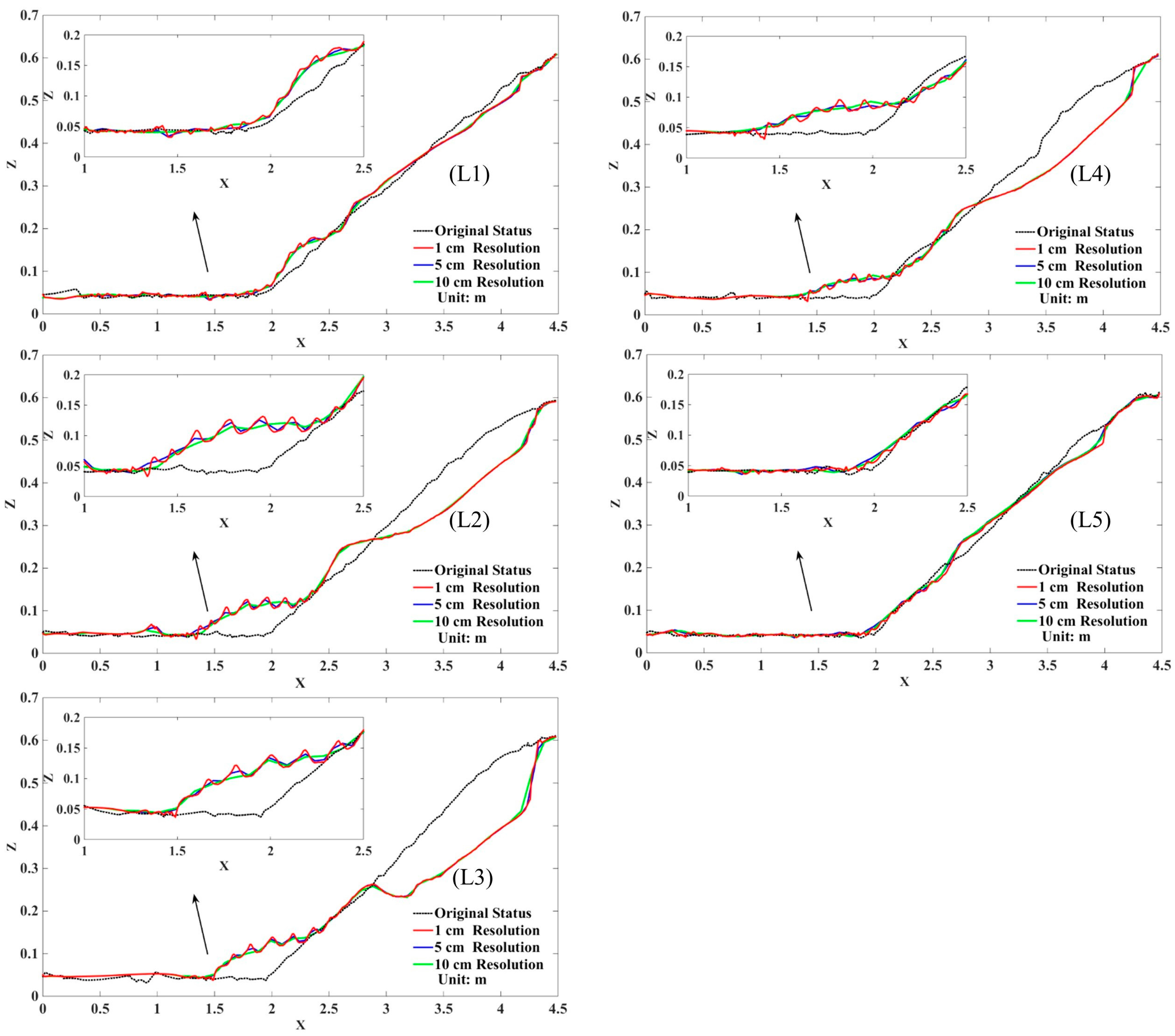
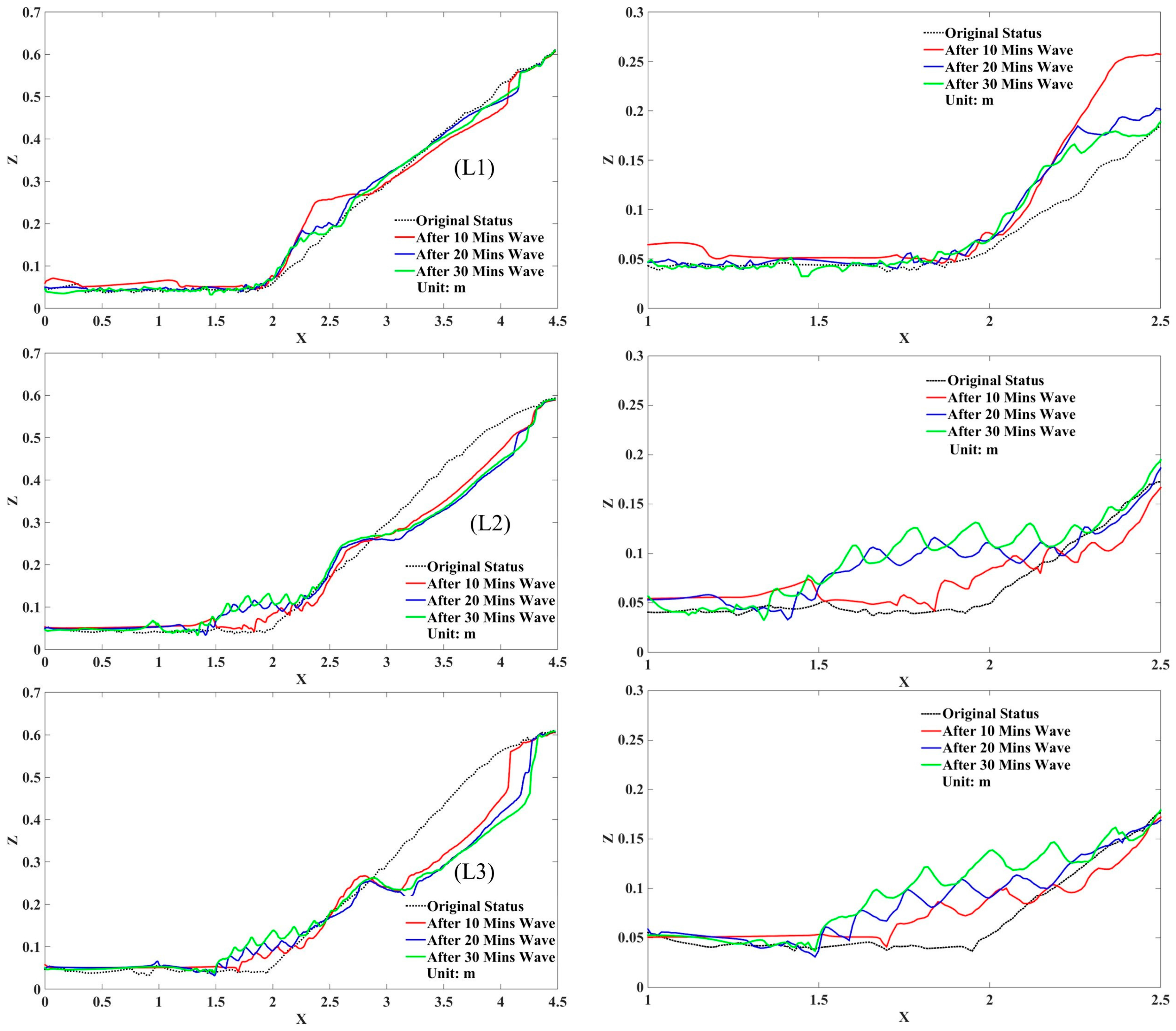
3.4. Assessment of Resolution Impact on Beach Profile Based on Sediment Change Analysis

Using beach models with 1, 5 and 10 cm resolutions, the impact of resolution on beach profile analysis can be examined in Figure 8. Profiles L1 and L5 lie close to the left and right edges of the wave tank, where relatively slight sediment changes occurred comparing to L2 to L4. Side effects can be observed further towards the wall through Figure 3d due to border effects. More distinguishable patterns were obtained at profiles L2, L3 and L4. Areas with relatively smooth surfaces resulted in less differences among profiles with different resolutions as demonstrated in the distance from around 2.5 to 4.2 m in L2, L3, and L4. However, those topographic features with peaks and troughs, smaller width, or abrupt slope changes could only be identified and accurately measured from the profiles derived from higher resolution models as shown in the areas with ripples (1.4–2.5 m) in L2, L3, and L4 and around 4.3 m in L4 and 3.9 m in L5.

To illustrate the application of fine-scale topographic mapping on beach evolution analysis, Figure 9 illustrates sediment change based on the beach model with the 1 cm resolution and profiles 1, 2, and 3 because of the symmetrical beach erosion patterns. The right column in Figure 9 demonstrates the capability of 1 cm resolution to detect subtle beach evolution patterns in sediment ripples. Major sediment erosion occurred at L2 and L3 between 3 and 5 m locations along the X axis, with most of this erosion occurring during the first 10-min wave application. Most of the sediment eroded in the upper areas was then deposited at immediately lower neighboring areas, between 1.5 and 3 m locations, forming obvious ripple patterns. Relatively fewer changes occurred at profiles L1, which was positioned along the edges of the wave tank.

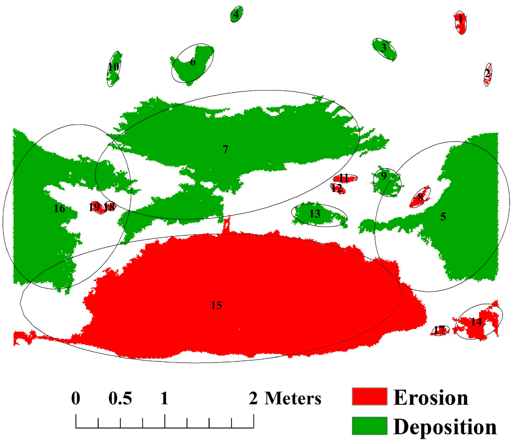
3.5. CMA Analysis for Sediment Change and Beach Evolution Assessment

Based on the elevation change map with 1 cm resolution in Figure 3, CMA identified a total of nineteen objects (ten erosional and nine depositional) outlined by fitted ellipses illustrated in Figure 10 with a focus on significantly changed areas over 2 cm in elevation and over a minimum of 50 pixels. Attributes of each object including location, area, volume, and object type are listed in

Table 1. Attributes of Objects Identified from CMA Sorted by Object Type and Volume.

Object ID	Object Type	Location-X (m)	Location-Y (m)	Area (m2)	Volume (m3)
15	Erosion	3.5	4.61	4.3522	0.393447
14	Erosion	6.36	3.62	0.0964	0.002408
1	Erosion	4.8	0.63	0.0214	0.000513
8	Erosion	5.19	2.61	0.0207	0.000495
11	Erosion	4.33	2.76	0.0142	0.000337
19	Erosion	1.92	4.2	0.0132	0.000334
17	Erosion	6.01	3.89	0.0111	0.000262
12	Erosion	4.3	2.9	0.0095	0.000224
18	Erosion	2.04	4.12	0.0076	0.000185
2	Erosion	5.32	1.04	0.0063	0.000137
7	Deposition	3.01	3.06	2.2086	0.09923
5	Deposition	5.5	2.71	1.1516	0.066502
16	Deposition	1.6	4.33	1.1699	0.057753
13	Deposition	4.23	3.26	0.099	0.002804
6	Deposition	2.23	2.28	0.1084	0.002502
9	Deposition	4.78	2.61	0.0674	0.001759
3	Deposition	4.14	1.25	0.0362	0.000977
10	Deposition	1.45	2.7	0.032	0.000846
4	Deposition	2.46	1.57	0.0173	0.000429

, which is organized by object type and volume. The location of each object was represented by the center coordinate of the corresponding fitted ellipse.

Table 2. Area Statistics of Erosional and Depositional Objects.

Object Type	Object Quantity	Sum of Area (m2)	Minimal Area (m2)	Maximal Area (m2)	Std. Deviation of Area
Deposition	9	4.8904	0.0173	2.2086	0.7861
Erosion	10	4.5525	0.0063	4.3522	1.3695

and

Table 3. Volume Statistics of Erosional and Depositional Objects.

Object Type	Object Quantity	Sum of Volume (m3)	Minimal Volume (m3)	Maximal Volume (m3)	Std. Deviation of Volume
Deposition	9	0.232801	0.000429	0.09923	0.0381
Erosion	10	0.398341	0.000137	0.393447	0.1242

summarize the statistics of sum, minimum, maximum and standard deviation of area and volume for the identified objects. The total erosional and depositional areas were 4.5525 m² and 4.8904 m², respectively. The erosional objects have a minimum area of 0.0063 m² and a maximum area of 4.3522 m²; while depositional objects have a minimum area of 0.2 m² and maximal area of 0.0173 m². The standard deviation of erosional objects (1.3695 m²) is approximately twice as that of the depositional area (0.7861 m²), indicating that the size of erosional objects varies more than the size of depositional objects. Meanwhile, the total erosional and depositional volumes are 0.398341 m³ and 0.232801 m³, respectively, ranging from minimum volumes of 0.000137 m³ and 0.000429 m³ to maximum volumes of 0.393447 m³ and 0.09923 m³. Erosional objects also vary more than depositional objects in terms of the volume due to a larger standard deviation. The average thickness of objects was calculated as total volume divided by total object area. For this experiment, the average thickness of erosional and depositional objects was 0.087 m and 0.048 m, respectively. Thus, the average thickness of erosional objects was almost twice that of depositional objects. These object-oriented statistics and geometry are demonstration of potential information that can be used for beach nourishment.

The results in Figure 11, Figure 12, Figure 13, Figure 14 and Figure 15 demonstrate the beach evolution based on CMA and beach models with 1, 5, and 10 cm resolutions. Figure 11, Figure 12 and Figure 13 showed that majority of the erosion and deposition were formed after the first period of wave application (P1). During the following periods of wave application, P2 and P3, drastically reduced areas and volumes of sand were eroded and deposited, but more ripple patterns were formed at the beach front. Overall, the beach was moving towards an equilibrium profile for the forcing conditions. When decreasing resolutions from 1 to 10 cm, the impacts of resolution were obvious from area statistics, reduced number of objects, and fuzzy boundaries. For 3D volume assessment, Figure 14 and Figure 15 demonstrate that the impacts on CMA-derived deposition volumes are minor when deposition areas are dominated by large areas. However, when the depositional objects are fragmented (such as P3), the impact of resolutions are significant (P2 is 62.1% of P1 and P3 is 39.7% of P1). This unexpected change is likely due to two factors: the minimum number of pixels for objects and ignoring insignificantly changed areas of less than 2 cm vertical difference.

4. Discussion

The main findings of this research include the following aspects. As terrestrial LiDAR technology develops and the cost drops, more users can afford to purchase these systems and the expense of use after the initial purchase will be comparable to other surveying instruments such as GPS. The research community often faces a common question: what is the uncertainty or accuracy for pre-processing when users apply the systems to various applications? This question is related to short- or long-range mapping and the surveying modes. The use of terrestrial LiDAR systems typically includes two modes: registration based on targets and registration based on point cloud mapping without targets. Target-based registration provides more reliable accuracy. As a short-range mapping technique using target-based registration, this research reported an accurate multi-site point registration process with a standard deviation of 0.009 m. When applying the system to multi-temporal topographic mapping, the uncertainties introduced by the multi-site registration and multi-temporal scanning are insignificant (−0.002 m ± 0.003), proving that terrestrial LiDAR systems are highly reliable for close range sediment change monitoring. In addition, close-range surveys based on two or more scanning sites produce a very high point density (more than 4 points/cm² in this experiment).

Given the increasing accessibility of topographic products of various resolutions (i.e., GDEM data from ASTER with 30 m resolution, airborne LiDAR with 0.5–5 m resolution, and terrestrial LiDAR and UAV maps with centimeter resolutions), users need to be aware of the impact of the resolutions on various sediment change analysis. This research focuses on the range within 10 cm resolutions for users with access to high density mapping. Within the 10 cm resolution range, all beach topographic models are capable of capturing major patterns of sediment erosion and deposition and perform comparably in areas with small slopes and smooth texture. However, topographic models with higher resolutions provide further detail in areas with rough surfaces, such as ripples and area with large slopes; models with coarser resolutions generally result in smooth effects with underestimated feature height (e.g., peaks and troughs) at rough surfaces and areas with steep slopes. What does this information mean for users? In potential applications, these small features or rough surfaces may represent surface cracks, signs of land subsidence or minor landslides of sand berms, severely eroded surfaces with abrupt slope changes, etc. If detecting these features as warning signs are important risk indicators or maintenance needs for specific applications, acquiring high-resolution mapping instruments or products is worthy of consideration. For volume estimation of sediment changes, decreasing the resolutions leads to an underestimation of erosional volumes and an overestimation of depositional volumes. These trends agree with the report from Woolard and Colby [29] based on resolutions of 1, 2, 5, 10, 15 and 20 m from aggregated airborne LiDAR data for coastal dune sites. In addition, both studies show that it is possible to have occasional resolutions slightly fall off the major trends such as the 0.05 m location in Figure 5. Decreasing the resolution from 1 to 10 cm resulted in a 2% underestimation of erosional volumes with a linear regression of y = −0.0964x + 0.4185 (R² = 0.9651) and a 3.5% overestimation of depositional volumes with a linear regression of y = 0.0664x + 0.3308 (R² = 0.3645). These regression models may be useful for users to predict and estimate the impact of resolution choices on pixel-based erosion or deposition volume assessments.

One practical and common need in sediment change analysis is to locate severely eroded areas and estimate sediment volume for nourishment of beaches, berms and levees, which have wide applications in wetland restoration, barrier island protection and levee monitoring. Compared to the commonly used sediment change analyses based on elevation change map, the recently developed CMA tool provides an effective yet simple approach to identify areas with significant erosion and deposition along with statistics on object-based attributes such as shape, area, volume, and thickness. As an application example for sediment change, CMA provides an effective tool for identifying the top four erosional objects (with volumes close to or more than 0.0005 m³) and the top three depositional objects (with volume larger than 0.057 m³, Table 1). When applied to outdoor environment, this information can support planning of beach nourishment to identify locations needed nourishment and their area and volume for cost assessment. When applied to multi-temporal beach evolution, CMA can provide a new perspective for sediment evolution analysis that differs from traditional pixel- and profile-based approaches. Users can specify a threshold of elevation change level for areas with obvious or severe sediment erosion and deposition, which correspond to areas of concern. The evolution patterns presented by the CMA method are simple and straight forward, which reduce the uncertainties introduced by different interpretations from users. The resolution impacts of topographic models are observable from the 2D beach evolution mapping through area, number, and the spatial distribution of detected objects. For volume assessment, resolutions have little impact on deposition volume with large objects and erosion volume. However, deposition volumes drastically decrease with resolution when fragmented objects dominant the statistics due to the minimum object size limit and ignorance of those less than 2 cm vertical difference. In addition, wave modeling experiments proved that resolutions of topographic models had substantial impact on wave height, free surface, and wave-introduced currents.

The limitations of this study are the scaling and border effects, similar to other wave-tank-based studies, which cause symmetrical sediment change patterns with a peak change near the center, gradually fading towards the borders. More experiments with different setups such as wave frequency can be implemented to simulate real-world scenarios as much as possible. However, this research focuses on evaluating topographic mapping based on terrestrial LiDAR and the impacts of resolution on sediment change analyses. The applications of the methods and parameters are developed for lab experiments and need improvement and adaptation when applied to fieldwork for future studies.

5. Conclusions

This research investigated the impacts of resolution of topographic mapping on various sediment change analyses including beach profiles, sediment erosion and deposition assessments, wave modeling, and object-oriented beach evolution. A Riegl VZ-1000 terrestrial LiDAR system conducted multi-site and multi-temporal survey of the exposed beach after three periods of wave applications in a laboratory setting. The system acquired dense survey data with more than 4 points/cm² and produced four beach models with an accuracy of −0.002 m ± 0.003. A set of high-resolution (1 cm) topographic products (e.g., topographic models, contour, slope, elevation change, and hill-shaded relief maps) illustrated the capability of the rapid and non-intrusive terrestrial LiDAR surveys to depict beach morphological features of various sizes on a detailed scale.

To study how the resolution impacts beach profile analysis, five profiles were derived from each of the 1 cm, 5 cm, and 10 cm resolution beach models. Results indicated that all of these resolutions were capable of capturing the major areas of sediment erosion and deposition, performing comparably in relatively smooth areas. However, differences appeared in areas with sudden slope changes and higher roughness such as the 3 cm wide sediment ripples. Detect small morphological features through high-resolution mapping is critical for potential applications such as surface crack detection and maintenance, beach and sand berm nourishment, wetland restoration, and detection of minor signs of surface displacement. The impact of resolution on volume change assessment was also studied by comparing the erosion and deposition volumes derived from a set of 10 beach models with resolutions from 1 cm to 10 cm at 1-cm increments. Changing resolutions from 1 cm to 10 cm resulted underestimation of erosional volume and overestimation of depositional volume, which agrees with the previous study based on airborne LiDAR data with resolution from 1 to 20 m. Two regression models can be used to predict the impacts of selected resolutions on erosional or depositional volume estimates. In addition, resolutions of topographic models had substantial impact on wave height, free surface, and wave-introduced currents.

Based on terrestrial LiDAR products, the object-based coastal morphological analysis tool CMA was applied to detect significant erosional and depositional areas. Nineteen objects were identified with location, area and volume attributes to support the distribution analysis of erosional and depositional objects. In addition, CMA was used to analyze the beach evolution after multiple wave applications. How erosion and deposition impacted the beach after each of the three 10-min periods of wave application was identified based on CMA analysis results. As an object-based morphological analysis, the ArcGIS Spatial Analyst extension tool CMA can analyze morphological change in aggregated areas and determine geometry and statistical attributes for each object, which is useful for identifying significantly eroded and deposited areas. The integration of terrestrial LiDAR and object-based morphological analysis was examined in a laboratory wave tank beach environment and found to be a successful method for identifying and analyzing wave-induced erosion and deposition.

References

1. Coleman, J.M.; Roberts, H.H.; Stone, G.W. Mississippi river delta: An overview. J. Coast. Res. 1998, 14, 698–716. [Google Scholar]
2. Morton, R.A.; Bernier, J.C.; Barras, J.A. Evidence of regional subsidence and associated interior wetland loss induced by hydrocarbon production, gulf coast region, USA. Environ. Geol. 2006, 50, 261–274. [Google Scholar] [CrossRef]
3. Kulawardhana, R.W.; Feagin, R.A.; Popescu, S.C.; Boutton, T.W.; Yeager, K.M.; Bianchi, T.S. The role of elevation, relative sea-level history and vegetation transition in determining carbon distribution in spartina alterniflora dominated salt marshes. Estuar. Coast. Shelf Sci. 2015, 154, 48–57. [Google Scholar] [CrossRef]
4. Kulawardhana, R.W.; Popescu, S.C.; Feagin, R.A. Fusion of lidar and multispectral data to quantify salt marsh carbon stocks. Remote Sens. Environ. 2014, 154, 345–357. [Google Scholar] [CrossRef]
5. Zhang, C.; Xie, Z. Data fusion and classifier ensemble techniques for vegetation mapping in the coastal everglades. Geocarto Int. 2013, 29, 228–243. [Google Scholar] [CrossRef]
6. Coops, H.; Geilen, N.; Verheij, H.J.; Boeters, R.; van der Velde, G. Interactions between waves, bank erosion and emergent vegetation: An experimental study in a wave tank. Aquat. Bot. 1996, 53, 187–198. [Google Scholar] [CrossRef]
7. Yuan, R.; Wu, X.; Luo, T.; Liu, H.; Sun, J. A review of water tank modeling of the convective atmospheric boundary layer. J. Wind Eng. Ind. Aerodyn. 2011, 99, 1099–1114. [Google Scholar] [CrossRef]
8. Masselink, G.; Pattiaratchi, C.B. Seasonal changes in beach morphology along the sheltered coastline of perth, western australia. Mar. Geol. 2001, 172, 243–263. [Google Scholar] [CrossRef]
9. Palmsten, M.L.; Holman, R.A. Laboratory investigation of dune erosion using stereo video. Coast. Eng. 2012, 60, 123–135. [Google Scholar] [CrossRef]
10. Erikson, L.H.; Hanson, H. A method to extract wave tank data using video imagery and its comparison to conventional data collection techniques. Comput. Geosci. 2005, 31, 371–384. [Google Scholar] [CrossRef]
11. Lippman, T.C.; Holman, R.A. Quantification of sand bar morphology: A video technique based on wave dissipation. J. Geophys. Res. 1989, 94, 17. [Google Scholar] [CrossRef]
12. Lippmann, T.C.; Holman, R.A. The spatial and temporal variability of sand bar morphology. J. Geophys. Res.: Oceans 1990, 95, 11575–11590. [Google Scholar] [CrossRef]
13. Holman, R.A.; Sallenger, J.; Asbury, H.; Lippmann, T.C.; Haines, J.W. The application of video image processing to the study of nearshore processes. Oceanography 1993, 6, 8. [Google Scholar] [CrossRef]
14. Astruc, D.; Cazin, S.; Cid, E.; Eiff, O.; Lacaze, L.; Robin, P.; Toublanc, F.; Cáceres, I. A stereoscopic method for rapid monitoring of the spatio-temporal evolution of the sand-bed elevation in the swash zone. Coast. Eng. 2012, 60, 11–20. [Google Scholar] [CrossRef]
15. Foote, M.; Horn, D. Video measurement of swash zone hydrodynamics. Geomorphology 1999, 29, 59–76. [Google Scholar] [CrossRef]
16. Holland, K.T.; Puleo, J.A.; Kooney, T.N. Quantification of swash flows using video-based particle image velocimetry. Coast. Eng. 2001, 44, 65–77. [Google Scholar] [CrossRef]
17. Mancini, F.; Dubbini, M.; Gattelli, M.; Stecchi, F.; Fabbri, S.; Gabbianelli, G. Using unmanned aerial vehicles (uav) for high-resolution reconstruction of topography: The structure from motion approach on coastal environments. Remote Sens. 2013, 5, 6880–6898. [Google Scholar] [CrossRef]
18. Zhao, K.; García, M.; Liu, S.; Guo, Q.; Chen, G.; Zhang, X.; Zhou, Y.; Meng, X. Terrestrial lidar remote sensing of forests: Maximum likelihood estimates of canopy profile, leaf area index, and leaf angle distribution. Agric. For. Meteorol. 2015, 209–210, 100–113. [Google Scholar] [CrossRef]
19. Meng, X.L.; Wang, L.; Silvan-Cardenas, J.L.; Currit, N. A multi-directional ground filtering algorithm for airborne LIDAR. ISPRS J. Photogramm. Remote Sens. 2009, 64, 117–124. [Google Scholar] [CrossRef]
20. Meng, X.L.; Wang, L.; Currit, N. Morphology-based building detection from airborne LIDAR data. Photogramm. Eng. Remote Sens. 2009, 75, 437–442. [Google Scholar] [CrossRef]
21. Meng, X.L.; Currit, N.; Zhao, K.G. Ground filtering algorithms for airborne LIDAR data: A review of critical issues. Remote Sens. 2010, 2, 833–860. [Google Scholar] [CrossRef]
22. Fairley, I.; Thomas, T.; Phillips, M.; Reeve, D. Terrestrial laser scanner techniques for enhancement in understanding of coastal environments. In Seafloor Mapping Along Continental Shelves: Research and Techniques for Visualizing Benthic Environments; Finkl, C.W., Makowski, C., Eds.; Springer International Publishing: New York, NY, USA, 2016; pp. 273–289. [Google Scholar]
23. Siadatmousavi, S.M.; Allahdadi, M.N.; Chen, Q.; Jose, F.; Roberts, H.H. Simulation of wave damping during a cold front over the muddy atchafalaya shelf. Cont. Shelf Res. 2012, 47, 165–177. [Google Scholar] [CrossRef]
24. Silva, R.; Baquerizo, A.; Losada, M.Á.; Mendoza, E. Hydrodynamics of a headland-bay beach—Nearshore current circulation. Coast. Eng. 2010, 57, 160–175. [Google Scholar] [CrossRef]
25. Silva, R.; Borthwick, A.G.L.; Taylor, R.E. Numerical implementation of the harmonic modified mild-slope equation. Coast. Eng. 2005, 52, 391–407. [Google Scholar] [CrossRef]
26. Ku, N.W.; Popescu, S.C.; Ansley, R.J.; Perotto-Baldivieso, H.L.; Filippi, A.M. Assessment of available rangeland woody plant biomass with a terrestrial LIDAR system. Photogramm. Eng. Remote Sens. 2012, 78, 349–361. [Google Scholar] [CrossRef]
27. Klemas, V.V. Coastal and environmental remote sensing from unmanned aerial vehicles: An overview. J. Coast. Res. 2015, 1260–1267. [Google Scholar] [CrossRef]
28. Liu, H.; Wang, L.; Sherman, D.; Gao, Y.; Wu, Q. An object-based conceptual framework and computational method for representing and analyzing coastal morphological changes. Int. J. Geogr. Inf. Sci. 2010, 24, 1015–1041. [Google Scholar] [CrossRef]
29. Woolard, J.W.; Colby, J.D. Spatial characterization, resolution, and volumetric change of coastal dunes using airborne LIDAR: Cape Hatteras, Horth Carolina. Geomorphology 2002, 48, 269–287. [Google Scholar] [CrossRef]
Figure 1. Bird’s-eye view of the initial experimental setup from the 3D data obtained by terrestrial LiDAR.
Ijgi 06 00147 g001
Figure 2. The initial beach has a slope of approximately 15°. Five beach profiles are distributed evenly with a cross-profile distance of 0.93 m.
Ijgi 06 00147 g002
Figure 3. (a) Hill-shaded relief map, (b) contour map (5 cm intervals) overlaid on DEM, (c) slope map and (d) map of elevation change.
Ijgi 06 00147 g003
Figure 4. Beach morphological models having resolutions of 10 cm (a), 5 cm (b) and 1 cm (c) with corresponding highlighted areas of erosion and deposition (d), (e), and (f) showing clarity of the area with the most sediment dynamics.
Ijgi 06 00147 g004
Figure 5. The impact of spatial resolutions on erosional and depositional volume estimates.
Ijgi 06 00147 g005
Figure 6. The wave modeling results derived based on 1 cm (A), 5 cm (B) and 10 cm (C) beach models. From top to bottom row are the wave height, instantaneous free surface, and currents, respectively.
Ijgi 06 00147 g006
Figure 7. The wave height profile along Y = 2.75 m for the modeling results based on beach models with 1, 5, and 10 cm resolutions.
Ijgi 06 00147 g007
Figure 8. Beach profiles L1 through L5 derived from topographic models with resolutions of 1, 5, and 10 cm. X is the distance in meters from beach front to areas with taller elevations. Z is the elevation value in meters. The zoom-in windows in these figures shows more detailed information about the ripple patterns in corresponding figures and the arrows serve as a reference to illustrate the same distance of 1.5 m.
Ijgi 06 00147 g008
Figure 9. Beach evolution analysis based on beach profiles L1 through L3 (left column), with L3 in the middle of the wave tank. The column on the right includes the plots of corresponding areas (1–2.5 m) with subtle differences.
Ijgi 06 00147 g009
Figure 10. CMA identified nineteen significant erosional and depositional objects highlighted by fitted ellipses.
Ijgi 06 00147 g010
Figure 11. Beach evolution based on CMA analysis and beach models with 1 cm resolution. The upper figures are beach models showing the initial model (a) and models after one (b), two (c), and three (d) periods of wave application. (e,f) show the changing areas of sediment erosion and deposition between consecutive beach models that occurred after one (e), two (f), and three (g) periods of wave application. Each period of wave application lasted 10 min.
Ijgi 06 00147 g011
Figure 12. Beach evolution based on CMA analysis and beach models with 5 cm resolution. The upper figures are beach models showing initial model (a) and models after one (b), two (c), and three (d) periods of wave application. (e,f) show the changing areas of sediment erosion and deposition between consecutive beach models that occurred after one (e), two (f), and three (g) periods of wave application. Each period of wave application lasted 10 min.
Ijgi 06 00147 g012
Figure 13. Beach evolution based on CMA analysis and beach models with 10 cm resolution. The upper figures are beach models showing initial model (a) and models after one (b), two (c), and three (d) periods of wave application. (e,f) show the changing areas of sediment erosion and deposition between consecutive beach models that occurred after one (e), two (f), and three (g) periods of wave application. Each period of wave application lasted 10 min.
Ijgi 06 00147 g013
Figure 14. Total erosion volume change assessment based on CMA analysis after three wave application periods.
Ijgi 06 00147 g014
Figure 15. Total erosion volume change assessment based on CMA analysis after three wave application periods.
Ijgi 06 00147 g015