
An Improved Hybrid Method for Enhanced Road Feature Selection in Map Generalization


1
College of Resources Environment and Tourism, Capital Normal University, Beijing 100048, China
2
3D Information Collection and Application Key Lab of Education Ministry, Capital Normal University, Beijing 100048, China
3
Beijing State key Laboratory Incubation Base of Urban Environmental Processes and Digital Simulation, Capital Normal University, Beijing 100048, China
*
Author to whom correspondence should be addressed.
ISPRS Int. J. Geo-Inf. 2017, 6(7), 196; https://doi.org/10.3390/ijgi6070196
Submission received: 20 April 2017
/
Revised: 28 June 2017
/
Accepted: 28 June 2017
/
Published: 1 July 2017
Abstract
:Road selection is a critical component of road network generalization that directly affects its accuracy. However, most conventional selection methods are based solely on either a linear or an areal representation mode, often resulting in low selection accuracy and biased structural selection. In this paper we propose an improved hybrid method combining the linear and areal representation modes to increase the accuracy of road selection. The proposed method offers two primary advantages. First, it improves the stroke generation algorithm in a linear representation mode by using an ordinary least square (OLS) model to consider overall information for the roads to be connected. Second, by taking advantage of the areal representation mode, the proposed method partitions road networks and calculates road density based on weighted Voronoi diagrams. Roads were selected using stroke importance and a density threshold. Finally, experiments were conducted comparing the proposed technique with conventional single representation methods. Results demonstrate the increased stroke generation accuracy and improved road selection achieved by this method.
1. Introduction
Road networks are the primary geographical feature comprising map skeletons. As a result, road network generalization has become an active area of research in map generalization [1,2,3]. Furthermore, road selection is one of the most important steps in road network generalization and a prerequisite that affects its accuracy. Road selection methods can be categorized, according to the network representation mode, into linear methods [4,5,6,7,8,9,10,11] and areal [12,13,14,15] methods.
Roads in a network are regarded as “streets” in linear methods, which select road segments by integrating graphic constraints. They are considered “blocks” in areal methods, which delete road segments by aggregating these blocks. Thomson and Richardson employed perceptual grouping using ‘good continuity’ to conduct road selection, in which individual road segments were grouped into continuous ‘straight’ lines [5]. Xu, Liu and Zhang utilized a linear method, which did not rely on the use of semantic data, to select roads based on a hierarchical structure [8]. Chen et al. proposed an areal approach to road selection, based on mesh density, which considered the topological, geometric, and semantic properties of road networks [15]. Linear methods have several advantages. They can be easily combined with graph theory and do not rely heavily on road attribute information. However, they are difficult to integrate with global statistical information from a road network, which can potentially lead to large deviations in selection results from different regions. In contrast, areal methods make full use of statistical information but tend to generate disconnected selection results. Selection accuracy depends primarily on attribute integrity and reasonable partitioning of a road network. Most conventional techniques use either a linear or areal method alone. However, single representation methods often suffer from low accuracy and biased structural selection. Several previous studies have demonstrated that a combination of both linear and areal approaches may improve performance [16,17,18]. Li and Zhou described an integrated approach to building hierarchical structures for road networks with a continuous multi-scale representation, in which linear and areal patterns were combined [16]. Benz and Weibel developed an algorithm for automated road network selection from a large-scale to medium-scale database, based on an extended stroke-mesh combination algorithm [17]. Liu, Zhan and Ai introduced a novel algorithm for road network selection in map generalization, based on stroke and Voronoi diagrams [18]. However, the linear and areal methods used in these studies still have some limitations. Hybrid methods need to be explored further as different combination strategies may result in varying selection accuracy.
Linear methods can be divided primarily into graph-based [19,20] and stroke-based [8,9,10,11] methods. Stroke-based methods are superior to graph-based methods in maintaining geometric continuity and a longitudinal hierarchy. However, stroke-based methods suffer from two common problems. First, when two road segments are connected as a stroke, connection rules can typically be established only if the deflection angle is less than the threshold value. This connection rule considers local aspects of the road segments but does not consider road segments with global connection rules. In other words, it lacks a global connection rule to establish a relationship between subsequent road segments and the initial road segment. Consequently, incomplete connection rules cannot satisfy the requirement that stroke-generated results exhibit significant overall continuity. Secondly, stroke-based methods often cannot generate global optimal or unique stroke results simultaneously with different stroke generation strategies. As such, the every-best-fit strategy could generate unique results, but it tends to converge to local optimum results. The self-best-fit strategy can achieve good global results, but it depends on initial road segments that typically involve a significant amount of uncertainty. Consequently, this approach often requires multiple iterations to achieve a tangible and satisfactory outcome. Nonetheless, road selection is based on global and unique stroke results. Local and uncertain stroke may affect final road selection accuracy, thereby impeding the practical application of stroke-based methods to road network generalization.
The areal method primarily uses road density as a threshold to control road selection [12,15]. Road density calculation methods include the grid [21], fractal [22], and mesh [15] methods. However, these techniques have some limitations. Specifically, the grid method tends to split road segments; the fractal method is difficult to use for determining initial grid size; and the mesh method relies heavily on the road network topology forming polygons. Previous studies have proposed the use of Voronoi diagrams to partition road networks [23]. The proposed technique overcomes the limitations of previous calculation methods and maintains information concerning road density. However, it neglects road weight when partitioning road networks based on ordinary Voronoi diagrams, which can delete important roads.
This paper presents an improved road selection method developed by combining the linear and areal methods together, with the intent of maintaining local details and the overall structure of the road network. More precisely, the stroke generation algorithm was designed to improve upon the linear method. A weighted Voronoi diagram was used to partition a road network in the areal method, which constrains road selection based on a density threshold. The remainder of this paper is organized as follows. Section 2 describes an improved method for road selection. In Section 3, the detailed process of road selection based on stroke and Voronoi diagrams is introduced. A case study is then developed to validate the proposed method in Section 4. Finally, Section 5 offers conclusions and suggestions for further study.
2. An Improved Method of Road Selection
We propose a new selection technique combining the linear and areal methods to avoid the limitations of using a single representation pattern. This approach improves the traditional stroke generation algorithm and builds a set of stroke evaluation indicators to constrain road selection from a local viewpoint. It also uses a weighted Voronoi diagram to calculate road network density and control road selection from a global viewpoint.
2.1. An Improved Stroke Generation Method
Strokes are composed of a set of road segments based on the principle of optimal continuity from perceptual grouping [5]. Stroke-based road selection methods primarily include two steps: stroke generation and stroke order. An accurate stroke generation algorithm is a prerequisite for effective stroke-based selection. In previous stroke generation methods, the initial road segment (used to generate the first stroke) and the new initial road segment (produced after generating a new stroke) were randomly selected. This brings into question the self-fit method and the self-best-fit method, which generated uncertain stroke results for the same road network. The every-best-fit method considers a deflection angle for each pair of road segments at one node and selects the most suitable road segment to connect with. This protects the method from random selection of an initial road segment and helps to generate unique stroke results. However, this connection strategy tends to terminate road segment connections, which can be continued to generate a single stroke. This may reduce the accuracy of road selection results, thereby impeding the practical use of stroke-based methods. To overcome this limitation, an overall stroke connection rule and a connection strategy based on road segment importance were designed to improve traditional stroke generation algorithms.
2.1.1. Overall Stroke Connection Rules
Stroke generation algorithms include connection rules and connection strategies. Connection rules determine whether road segments can be connected, while connection strategies specify how to connect road segments. Connection rules include geometric rules, attribute rules, and a mixed rule regarding geometry and altitude [24]. In practical applications, it is difficult to collect complete road attributes, such as road rank and name, while geometric information can be obtained from road networks directly. As such, most studies use geometry as a connection rule to constrain stroke generation.
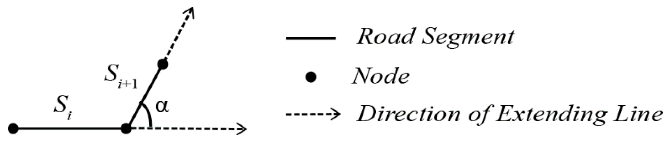
The “good continuity” principle proposed by Gestalt is often used as a guide to establish geometric connection rules [5]. Since the principle relies on human visual perception, it is difficult to quantify. Nevertheless, the deflection angle of road segments is often used only as an indicator to establish connection rules in most studies [8,9,10,11,25]. Based on the local indicator, two road segments can be connected on the condition that their deflection angle is less than a specified threshold. The deflection angle represents the degree of a deviation formed by two linked road segments, which ranges from 0° to 180°. This is depicted in Figure 1, where α is the deflection angle of road segment Si and Si+1.
However, the deflection angle only represents local road segment information and does not reflect their overall relationship. Not only is the deflection angle utilized, it must also consider the relationship between subsequent and initial road segments [26]. In other words, it is necessary to constrain the relationship between initial road segments and subsequent connections to minimize bias. An extension of the overall direction is a criterion for visual stroke generation. As such, the overall direction needs to be considered in the stroke generation process. Additionally, it is important to maintain overall spatial distribution characteristics with the original road network. In the proposed method, strokes were chosen as the basic unit of road selection. As such, stroke results directly affect road network selection accuracy. However, local stroke results cannot meet the requirements of maintaining overall road network characteristics, thereby reducing road selection accuracy.
Ordinary least squares (OLS) is a parameter estimation model that produces the line of best fit for a set of data by minimizing the square of the residuals. The declination rate for the fitting line represents the overall directional information for these scatter points. Similarly, based on road nodes, declination rates for road segments can be calculated using the OLS model, which provides overall directional information for road segments. The declination rate and deflection angle were chosen as indicators to design stroke connection rules. Particularly, the declination rate is an overall information indicator, representing deflection angle and local information for connected road segments. Essentially, a stroke is a continuous path composed of several road segments. The declination rate of a path was calculated using the OLS model with nodes present along a path. It can then characterize initial road segments with subsequent segments. After introduction of the OLS model, overall road segment information was considered and a comparison was made between the deflection angles within a threshold. This translated into a comparison with the declination rate. Hence, changes in computational efficiency led to negligible differences. Furthermore, stroke generation accuracy can be advanced without decreasing efficiency. Therefore, the declination rate can be used as a connection rule to control stroke generation.
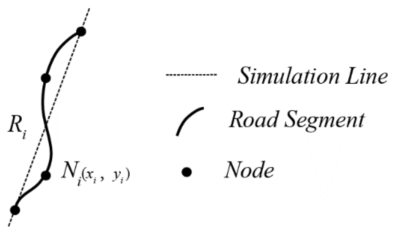
As can be seen in Figure 2, the path Ri is composed of Ni (i = 1,2,...,n) nodes and n − 1 road segments. The (xi, yi) terms represent the coordinates of nodes Ni, while the declination rate m of path Ri was calculated using the following equation:
where and represent the abscissa and ordinate averages for the n nodes, respectively.
This paper proposes a connection rule for stroke generation by combining local and global rules. Specifically, the connection rules are as follows: (1) from a local viewpoint, the deflection angle is less than the angle threshold value θ. As is known from previous studies, θ is typically less than 60° [10,25]. (2) From an overall viewpoint, the OLS model was used to calculate a declination rate and road segments featuring the minimum difference value with initial segments were chosen as connected road segments. This was done so the stroke could have good continuity as a whole.
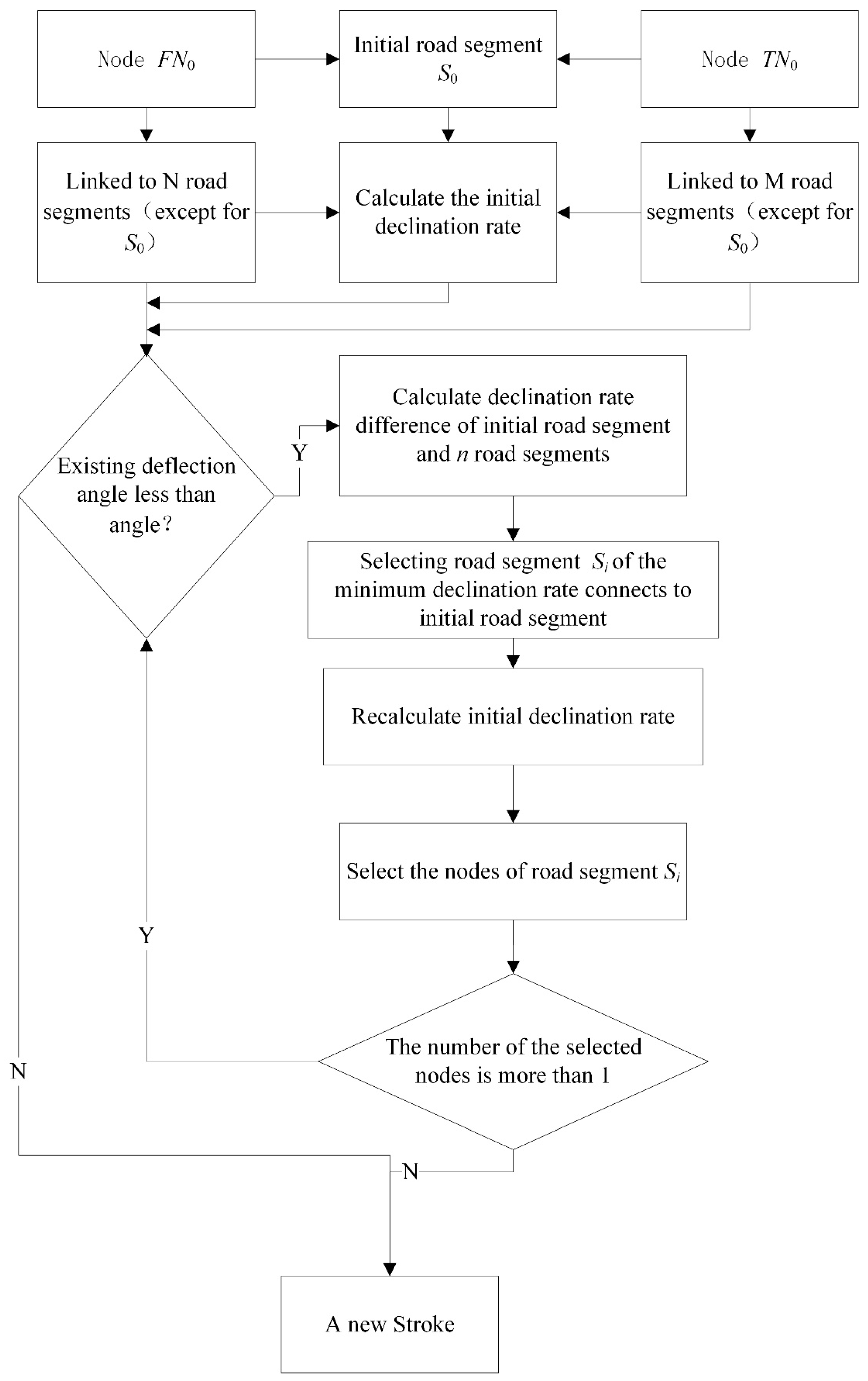
A connection rule flowchart is shown in Figure 3. Supposing that nodes FN0 and TN0 are nodes for the initial road segment S0, the number of road segments generated by the stroke from e node FN0 (which satisfy the first connection rule at node FN0) is n. The declination rate for an initial road segment S0 is m0, where mi (i = 1, 2, …, n) is the declination rate of paths formed by the n road segments linked to node FN0. If Δm = min |mi − m0|, the road segment Si corresponding to Δm is connected to the initial road segment S0. Before carrying out the next connection, new declination rates were set to the initial declination rate, namely m0 = mi. Road segments linked to the nodes at road segment Si continue being updated using connection rules (1) and (2) until there is no road segment satisfying the first connection rule. A new stroke is then generated using the same method, processing the other nodes TN0.
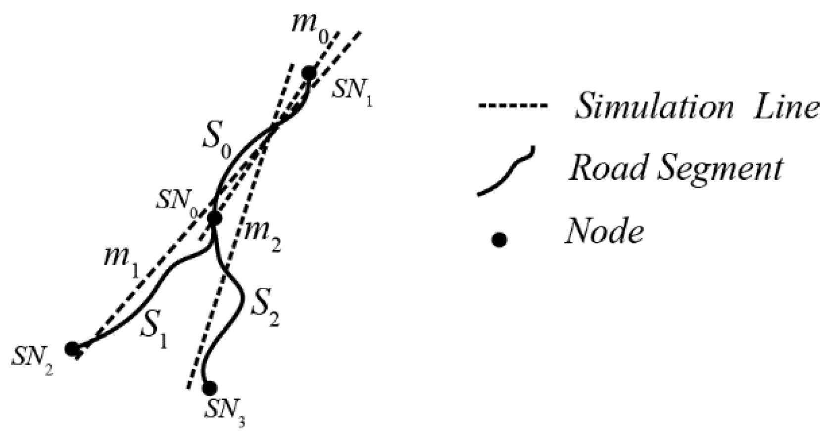
Figure 4 demonstrates the proposed algorithm. As shown in the figure, road segments S0, S1, and S2 are linked to node SN0. Supposing that a stroke was generated from road segment S0, the deflection angles S1, S2, with S0, were calculated, respectively. Declination rates for nodes (SN1, SN0), (SN1, SN0, SN2), and (SN1, SN0, SN3), were m0, m1 and m2, respectively. The following three situations could potentially occur when generating a stroke at node SN0: (1) if both of the deflection angles are less than θ, the absolute value of the difference of m1 with m0 and m2 with m0 was calculated, respectively. Without loss of generality, we assumed |m1 − m0| < |m2 − m0| and that road segment S1 was selected to connect with road segment S0. We then set m1 as the initial declination rate before connecting the road segments linked to node SN3; (2) if neither of the deflection angles are less than θ, the stroke generation algorithm is terminated at node SN0; (3) if only one road segment’s deflection angle is less than θ, the road segment can be directly connected with road segment S0.
Arc compression (i.e., the Douglas–Peucker algorithm) is a common processing method for curved road segments which obtains key points and calculates the overall curve direction before generating strokes. Ring road segments can be identified and pre-processed. First, ring patterns must be identified and the road segments removed. Reconnected road segments that were disconnected due to deletion of rings based on the road direction then form new road segments [17]. Finally, these road segments can be connected as strokes using the proposed stroke generation method.
2.1.2. A Connection Strategy Based on Road Importance
In many studies, the connection strategy is such that selection is randomized for initial and new road segments after stroke generation. The resulting strokes often include a significant amount of uncertainty for the same road network and require iterative stroke generation to improve results, which can decrease the efficiency of road selection. According to the reference [24], a connection strategy is set based on road importance to generate strokes. While this strategy can produce unique results, it primarily involves the use of local information and the indicators used to calculate road importance are overly complex, reducing stroke generation efficiency. Since connection rules have been designed by combining local and global road information (road importance is only used to sort road segments), the indicators of road segment importance can be simplified to improve the efficiency of stroke generation algorithms. As mentioned above, road rank and other road attributes are difficult to obtain in practice. Geometric road characteristics and other topological considerations (i.e., segment length and the number of roads linked with a segment) were chosen as indicators to calculate road segment importance. Longer road segments with a significant number of links were intuitively assigned greater importance. Calculation of this parameter was conducted as follows:
where and are the length of road segment i and the maximum length of all road segments, respectively; and are the number of road segments connected with road segment i and the maximum number of connected road segments; a and b represent the weight of length indicators and the connection number indicator, respectively.
2.2. Stroke Order Based on Stroke Importance
Calculating stroke order requires evaluating the importance of a stroke after it is generated. As this is critical to road selection, stroke order is a crucial step in stroke-based methods. The technique used to calculate stroke importance includes a regulation parameter generation, and weight-based method, which is a common approach to assigning indicator weights. Hence, constructing comprehensive and rational indicators is a precondition to evaluating stroke importance. From a combination of global and local viewpoints, stroke closeness and betweenness can be used as global indicators based on a dual graph. Stroke length and degree can be used as local indicators selected by integrating indicators used in previous studies. Specific calculation methods for evaluation indicators are shown in Table 2. These were weighted using the CRITIC method [27], which considers not only the nature of the indicator itself, but also considers the effects of interaction between different indicators. The equation for stroke importance is as follows:
In Equation (3), the weight p1, p2, p3 and p4 can be obtained using the CRITIC method; , , and are the maximum stroke length, degree, similarity, and closeness, respectively.
Objectively distinguishing the importance of stroke indicators is so difficult that it is necessary to calculate the weight of each stroke indicator based on the road network data itself. CRITIC is an objective weighting method that considers not only the internal differences of evaluation indicators themselves but also the relevance of various indicators. A primary contribution of the proposed technique is the determination of each indicator weight based on contrast intensity and conflicting indicator characteristics [24]. We first developed a standardization process for stroke evaluation indicators using the following equation:
where is the new value of the stroke evaluation indicator (which has been normalized); is the original value of the indicator; and represent the maximum and minimum of , respectively.
Secondly, we calculated the amount of information in each evaluation indicator:
where Cj is the amount of information in indicator j; is the standard deviation of indicator j; m is the number of stroke evaluation indicators, and represents the linear correlation coefficient of indicators j and k.
Finally, the weight of each stroke evaluation indicator was calculated based on the amount of information contained in the indicator using the following:
2.3. Road Density Based on a Weighted Voronoi Diagram
Although stroke-based methods consider the geometry and topology of a road network, they tend to ignore global density constraints, which increases the density difference in various spatial regions and leads to an unreasonable spatial structure in road selection results. In order to maintain correct spatial structure, road density must be calculated by partitioning the road network. This is a basic constraint commonly used in areal methods. As such, the chosen partition method greatly influences the resulting road selection. In light of the disadvantages of existing partition methods, an ordinary Voronoi diagram was introduced to partition road networks and calculate road density [23]. The proposed method could compensate for flaws in previous partition methods and maintain the overall spatial structure of a road network. However, ordinary Voronoi diagrams do not consider road importance when partitioning a road network. This could lead to the deletion of important roads under the constraints of the density threshold.
Figure 6 depicts the road partition density respectively using a weighted Voronoi diagram (Figure 6a) and an ordinary Voronoi diagram (Figure 6b). The darker the color, the higher the road density in the partition. Taking road segment RS as an example, its density is 35.2 (km/km2) and 23.1 (km/km2) based on an ordinary Voronoi diagram and a weighted Voronoi diagram, respectively. Under the control of the density threshold 25.5 (km/km2), road segment RS was deleted using an ordinary Voronoi diagram, while it was selected using the weighted Voronoi diagram. It can be seen from Figure 6 that the road segment RS in the road network plays a very important role in connectivity, and therefore it needs to be selected. In fact, weighted Voronoi diagrams take the road importance into account, as important roads occupy a larger area and thus result in lower road density. Therefore, an important road tends to be selected based on a weighted Voronoi diagram, which shows that a weighted Voronoi diagram is more reasonable than an ordinary Voronoi diagram in partitioning a road network.
Hence, it is necessary to generate a weighted Voronoi diagram to partition the road network according to the importance of a road segment. Road segment importance is calculated using Equation (2). The generation algorithm of a weighted Voronoi diagram was developed by [28]. Each segment partition area is obtained using a weighted Voronoi diagram because each road segment is used as a generation cell. However, stroke is considered to be a selected unit in this paper, so stroke density is defined as the ratio of total road segment length to total partition area for a given stroke. On the basis of partitioning a road network, stroke density is calculated as follows:
where represents stroke density; is the total partition area of stroke i; and is the length of stroke i.
As the most reasonable density threshold may vary with different cases, the empirical study method is often employed to determine density threshold by artificially analyzing the density distribution of the existing maps at different scales. However, the different scales of the road network data are difficult to obtain in actual applications, especially for non-basic scales. Li and Openshaw proposed the concept of Smallest Visible Object (SVO) based on ‘Natural Principle’ [29]. For maps at a certain scale, there must be a minimum road segment length for an area partition unit below which the road segment cannot be perceived any longer. Correspondingly, there must be a threshold of road density below which the road segment cannot be selected. Such a road density threshold is considered to be the largest permissible density.
A density threshold was employed to control the density distribution of a selected road network, based on that of the original road network. This density threshold was calculated as follows [15]:
where and are the scale factors of the target map and source map, respectively. The term represents the size of the smallest visible object (SVO) in terms of map distance.
Previous studies have recommended a value between 0.5 and 0.7 mm for Lm [29,30]. Müller also suggested a value of 0.4 mm as being appropriate [31]. Considering the scale of the target map (1:50,000) and source map (1:10,000), a value of 0.4 mm was chosen to calculate the road density threshold, which equals 25.0 (km/km2) based on Equation (8).
3. Road Selection Based on Stroke and Voronoi Diagrams
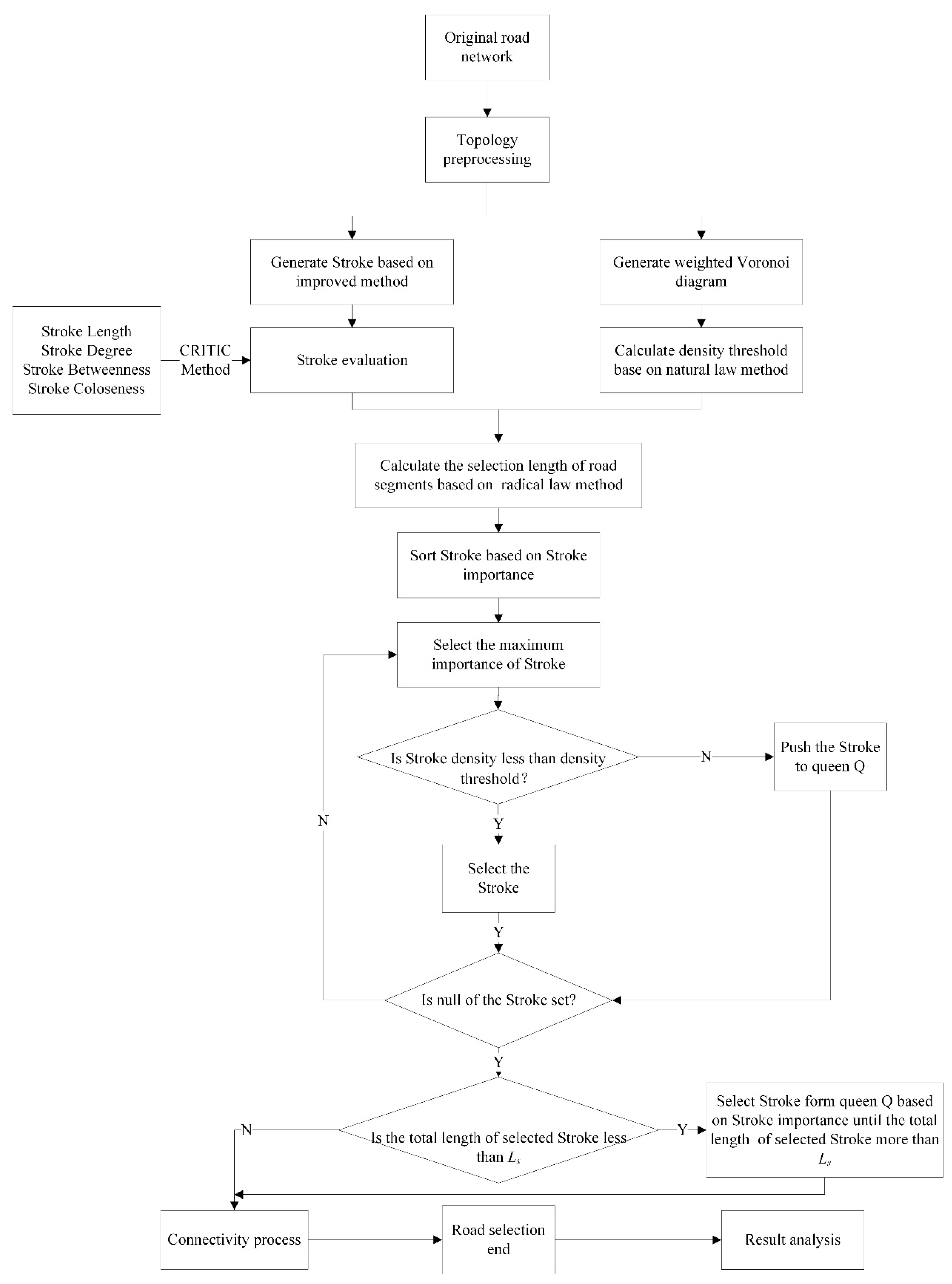
There are three parameters which need to be considered during the process of road selection, namely, stroke importance (SI), stroke density threshold (DS), and length of the selected network (LS). The SI parameter does not need any threshold constraints and DS can be obtained using Equation (3). LS is calculated by multiplying the number of selected road segments and the average length of the original road network. The number of selected road segments can be determined from the reference [32]. Under the control of the DS and LS parameters, roads are selected according to the order of SI from high to low. In the majority of previous studies, road structure selection is based solely on road importance, which might result in the unreasonable spatial structure as well as the irrational spatial distribution of road density. Therefore, stroke importance and density threshold were used to select roads based on the improved stroke generation method and a weighted Voronoi diagram. Figure 7 shows the overall process of road selection used in this paper. The detailed algorithm process is as follows:
- (1)
- Generate a stroke using the improved stroke algorithm and compute stroke importance using the CRITIC method based on the evaluation indicators in Table 2. Then sort strokes based on stroke importance.
- (2)
- Generate a weighted Voronoi diagram to partition the road network and calculate stroke density based on the partition. Then calculate a density threshold using the natural principle method.
- (3)
- Calculate the total length Ls of the road selection using the radical law method.
- (4)
- Make stroke a selection unit used to select road segments based on stroke importance as well as stroke density. The strokes were sorted based on stroke importance and selected the strokes according to order, from high to low. If a stroke density is lower than the density threshold, the stroke is selected. The selected algorithm continues until the total length of the selected stroke is larger than Ls. If the total length of the selected stroke is still smaller than Ls when all strokes are processed using the selected algorithm, the strokes whose densities are lower than the density threshold are continually selected based on stroke importance until the total length of selected strokes is larger than Ls.
- (5)
- If the selected road network is disconnected, then a minimum spanning tree method is used to connect the road network by adding a minimum number of nodes [33]. In order to ensure overall connectivity of the road network after selection, the shortest path is selected to connect pseudo nodes to newly added nodes until all pseudo nodes have been processed.
4. A Case Study
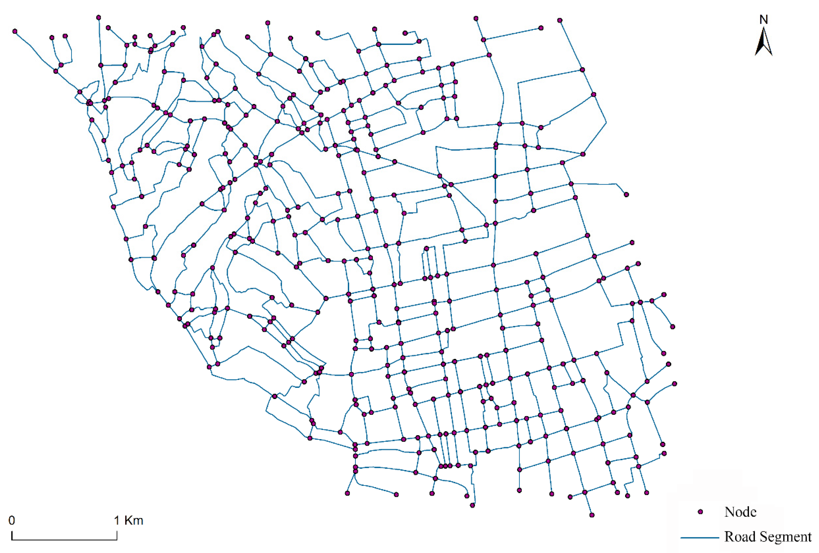
Road network data were acquired from the national land investigation of China for test purposes. The study area covered 21.5 km2 and was located in Neixiang County in Henan Province. As shown in Figure 8, the data scale was 1:10,000 and there were 422 nodes and 644 road segments. The total length of all road segments was 152.1 km.
The experiment was conducted within an integrated C# environment running ArcEngine10.1 on a Windows 8 operating system with a CPU Intel Xeon E3-1226 processor at 3.30 GHz. The detailed experimental process followed the algorithm procedure described in Section 3. The accuracy of road selection and stroke generation were computed using the following equation:
where MR and AR represent manual results and algorithm results, respectively. The IR term represents identical outcomes between manual and algorithm results. The resulting road selection and stroke generation data were used to quantify algorithm performance, as described in the following sections.
4.1. Analysis of Stroke Generation Results
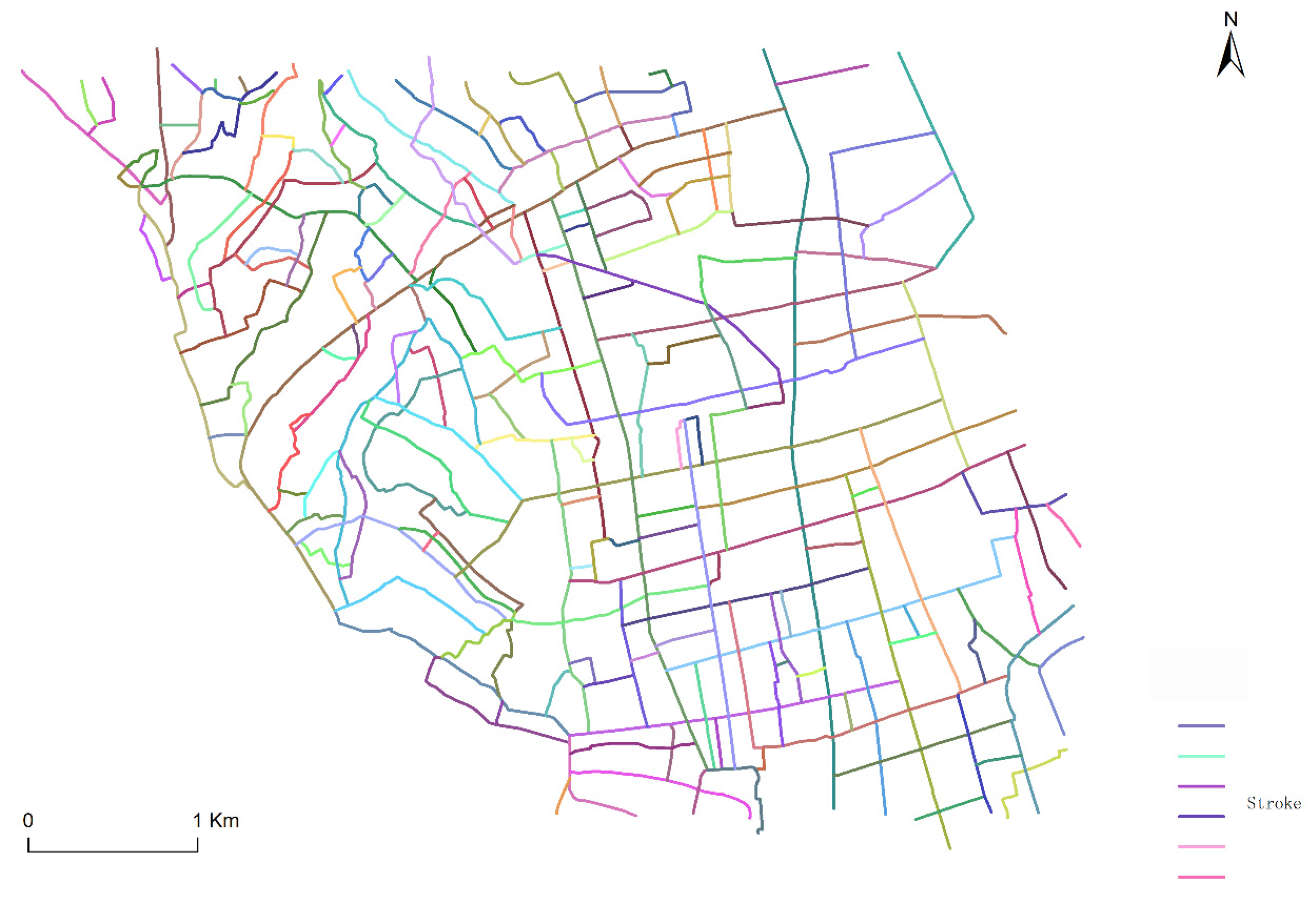
Figure 9 shows stroke generation results based on an improved stroke generation algorithm, with 189 strokes rendered in different colors. Local stroke results are shown in Figure 10. As can be seen in the figure, road segment s is the initial road segment, and road segments a, b and c are linked with node ND, where road segment b and c are to be connected. The deflection angle of road segments a and b and that of a and c were 35° and 31°, respectively. Both deflection angles were less than the established angle threshold of 60°. It is evident that road segment c was selected to connect to road segment a using the traditional stroke generation algorithm, since 31° is less than 35°. After introducing the OLS model, a declination rate difference was calculated between the initial road segment s and the path after connecting road segments a and b and a and c. These declination rates were found to be 0.07 and 0.25, respectively. As 0.07 is less than 0.25, road segment b was selected to connect road segment a using the improved stroke generation algorithm. It is visually apparent in Figure 10 that the connection of road segments a and b with the initial road segment s achieves better overall continuity than that of segments a and c. Unlike the traditional stroke generation algorithm (based solely on local deflection angles), the improved stroke generation algorithm considers the relationship between initial and subsequently connected road segments.
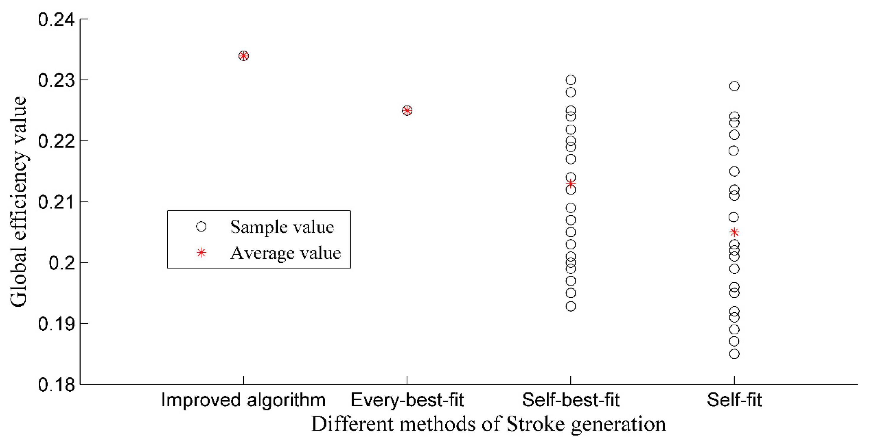
The global efficiency of a network describes the degree of smoothness for information dissemination in the network and can be used as an indicator to evaluate global strokes. A larger value indicates a better global stroke and vice versa. The global efficiency can be calculated as follows [24]:
where N is the total number of road segments, and is the minimum number of road segments from node i to node j.
The traditional stroke algorithm refers to the self-fit, every-best-fit, and self-best-fit methods. Every-best-fit requires that each pair of segments at a junction point negotiate with each other to achieve the best fit. In the process of the self-best-fit, each segment only considers itself, and neglects the others. The self-fit arbitrarily chooses one fit to join under the threshold control of the deflection angle, but not necessarily to be the best fit. We conducted 20 experiments and acquired results using different stroke generation methods, the results of which are shown in Figure 11. As can be seen in the figure, both the improved method and the every-best-fit method produced unique stroke results each time, but the global efficiency of the improved method was higher than the every-best-fit method. As the influence of initial road segments is randomly chosen, stroke results for the self-best-fit method and the self-fit method always differed from each other. The maximum, mean, and minimum values of the global efficiency for the two methods were smaller than those of the improved method, while the variance is greater than that of the improved method. Compared with the traditional stroke generation method, the improved method achieves the best global stroke results.
In this paper, traditional stroke generation methods were selected to compare with the improved stroke method using a statistical test. In order to minimize the influence of subjective factors, strokes were used as a benchmark to compare different methods and were integrated into the generated results by experienced cartographers. We randomly selected 100 and 200 nodes from the Neixiang case data to measure the stroke type at each node. Any results that were the same as the manual stroke at a given node were defined as the correct type; otherwise, they were considered to be an error. The statistical results acquired using different stroke generation methods are shown in Table 3, which demonstrates that the improved method achieved the highest accuracy. Table 4 includes chi-square values of 13.8 and 24.7, which are both larger than the test value: (7.82) for three degrees of freedom. Moreover, each featured at a significance level of 0.05, which demonstrates the significant differences between stroke results obtained by varying methods. The procedure proposed by Marascuilo was employed to further examine differences between the improved and traditional stroke methods [16]. The results are shown in Table 5. Absolute difference denotes proportional differences between the comparison methods, and the critical range is the test value obtained using the Marascuilo procedure. The difference is statistically significant if the absolute difference is greater than the corresponding critical range. As can be seen in Table 5, the absolute difference was greater than the critical range. As such, the proposed method significantly improved stroke accuracy.
4.2. Road Density Result Analysis
Theoretically, the mesh is abstracted based on an enclosed area surrounded by road segments. Therefore, the mesh density can only involve road segments whose topology can construct areal features. A weighted Voronoi diagram covers such shortages and can be used to calculate road density for all types of road networks by partitioning a network into subareas. Strokes were selected according to the order of stroke importance from highest to lowest, rather than being deleted from low to high. As can be concluded from the algorithm flow, this determines whether a stroke is selected but cannot determine whether a stroke is deleted. Therefore, dynamic calculation of road density has little effect on the final road selection results. We acquired 150 areal road segments from the Neixiang study to compare road selection results using weighted Voronoi diagrams and the mesh method. The latest issue of the 1:50,000 road map of the Neixiang case was selected as a benchmark. This road selection with benchmark data was considered to be the correct selection, otherwise it was considered a false selection. The final selection accuracies of the weighted Voronoi diagram and mesh methods were 83.6% and 82.7%, respectively. There was little observed difference between the accuracy of these two methods.
Figure 12 shows a comparison between the weighted Voronoi method and the mesh method. Figure 12a is a schematic road network with areal road segments. As can be seen in Figure 12b, the density of meshes 1–4 are decreasing. Under the control of the density threshold, mesh 1 and 3 were merged into mesh 1–3; mesh 2 and 4 are merged into mesh 2–4; mesh 1–3 and mesh 2–4 were merged into mesh 1–2–3–4. It can be seen in Figure 12c that the density of road segments st1, st2 and st3 are decreasing. Based on a given density threshold, road segments st1, st2 and st3 may not be selected. Therefore, it can be concluded from the road selection process that the weighted Voronoi diagram and the mesh method achieved essentially the same results for the road network with ordinary areal road segments. During the process of road selection, the mesh method needs to fully consider adjacent meshes, while the weighted Voronoi diagram directly compares the road density with a density threshold to determine whether a road segment is selected. The weighted Voronoi diagram method offers a simple calculation process (nearly equivalent to the selection accuracy) whose implementation is simpler than the mesh method.
Road networks that contain both linear and areal segments belong to the hybrid road network pattern [16], as shown in Figure 12d–f, which show selection results for the mesh method and weighted Voronoi method. It is evident in the figure that the mesh method only considers areal road segments. It is therefore unreasonable to apply hybrid road patterns, as linear road segments are unable to form a mesh and thus lead to biased selection results.
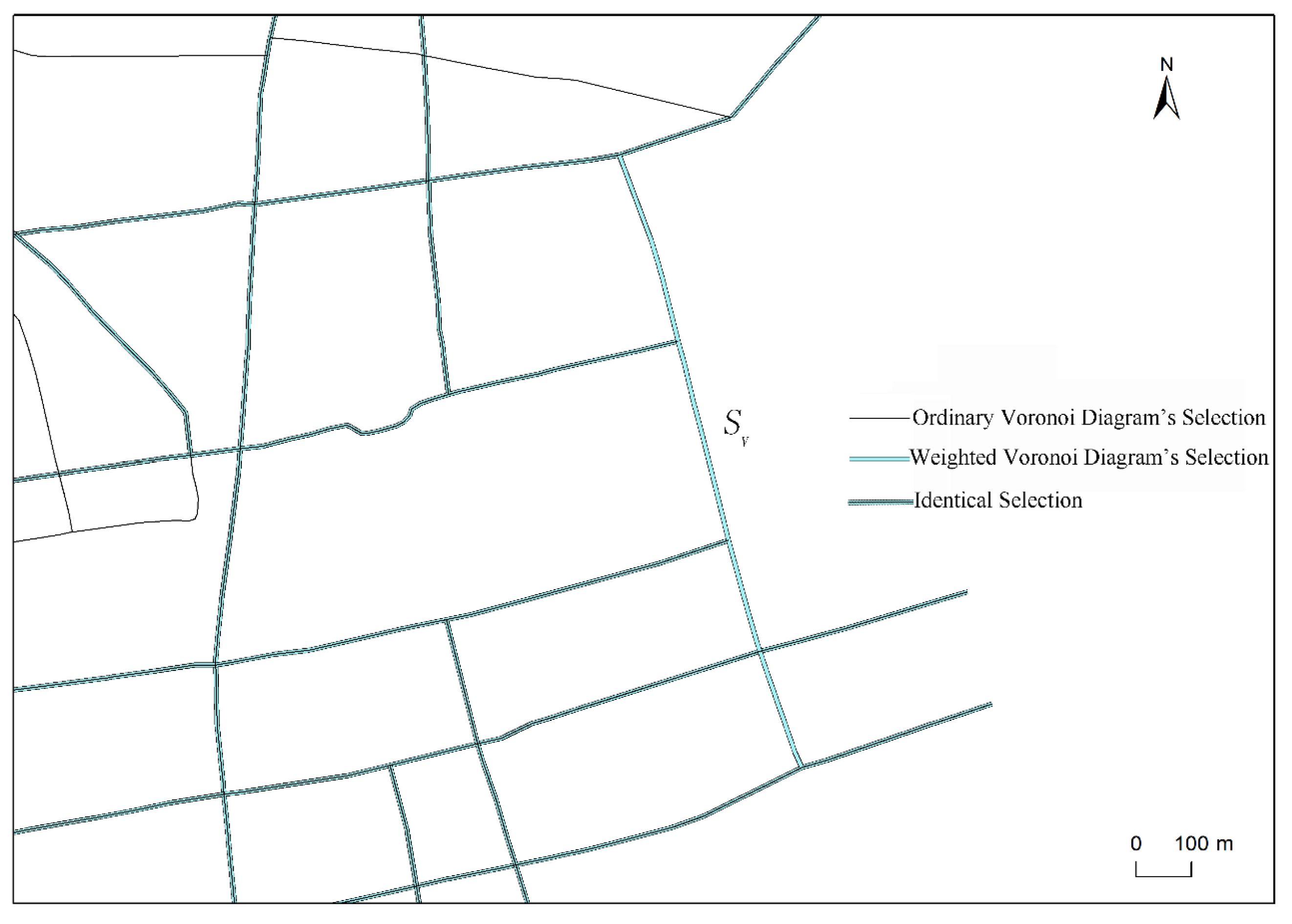
Figure 13 is a local comparison of selection results between the ordinary Voronoi diagram and a weighted Voronoi diagram. As shown, stroke Sv is composed of four road segments but was deleted based on ordinary Voronoi diagram partition, because of density threshold limitations. In contrast, stroke Sv was selected in the process of the weighted Voronoi diagram partition, because the importance degree of stroke Sv was large and the density was larger than the threshold. Stroke Sv was also selected by manual selection because it links several road segments and plays an important role in road network connections. In Neixiang case, the final selection accuracy of the weighted Voronoi diagram and the ordinary Voronoi method were 85.8% and 80.2%, respectively.
4.3. Results Analysis for Road Selection
As a benchmark for comparing different stroke generation methods, the manual selection of strokes still includes some degree of uncertainty, regardless of the combination of cartographic experts. In order to study the effect of different stroke generation methods on road selection, an additional two study cases which are part of the road network data of Tianjin and Shanghai were selected, except for the Neixiang case. First, four different stroke generation methods were used to obtain corresponding strokes in three different cases. These strokes were then selected based on the proposed road selection algorithm in this paper. Finally, road networks of 1: 50,000 in the three study areas were obtained using different stroke results. The map data, which were officially issued at the same period with the case data, were chosen as a benchmark. The statistics of the final road selection results based on different stroke methods are shown in Table 6. It can be seen from Table 6 that in three study areas, the improved stroke method performs the best and the selection accuracy of the road network exceeds 85%. As for the traditional three-stroke generation methods, the accuracy difference of the self-best-fit and self-fit methods varies significantly in different study areas, since the stroke results of the two methods are uncertain.
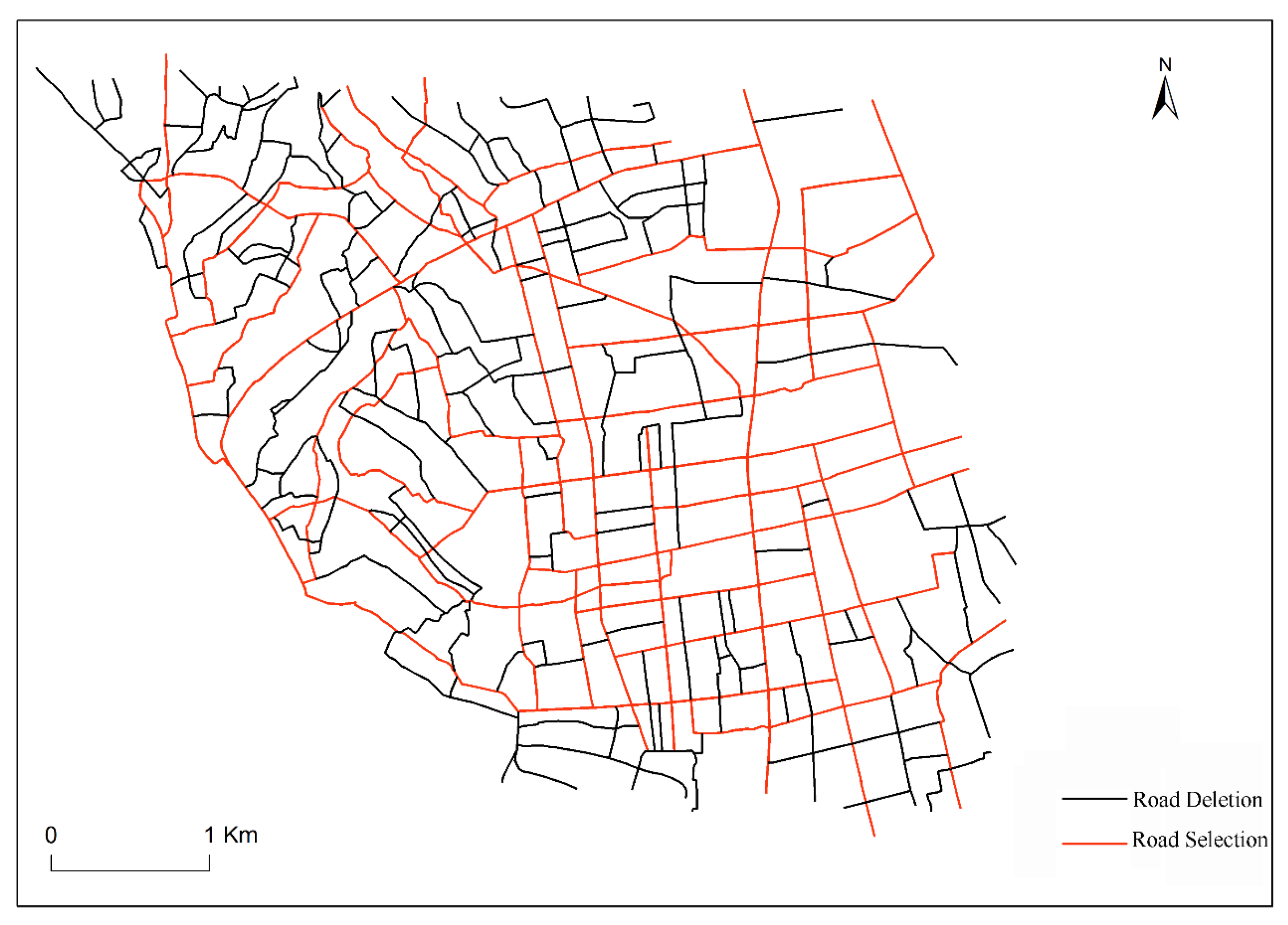
The results of the proposed method are shown in Figure 14. It is evident this method leads to accurate road selection results which maintain the overall structure of the road network and are also reasonable in different regions. In order to verify the results of the improved road selection method, the single method, namely stroke-based and mesh density-based methods, were selected to compare with the improved method based on manual selection results. These results are shown in Table 7. It is obvious the road selection accuracy of the improved method is highest among the three selected methods, and it increases by 8.1% and 10.3% compared to the stroke-based method and mesh density-based method, respectively. As a result, the improved method increases the overall accuracy of road selection.
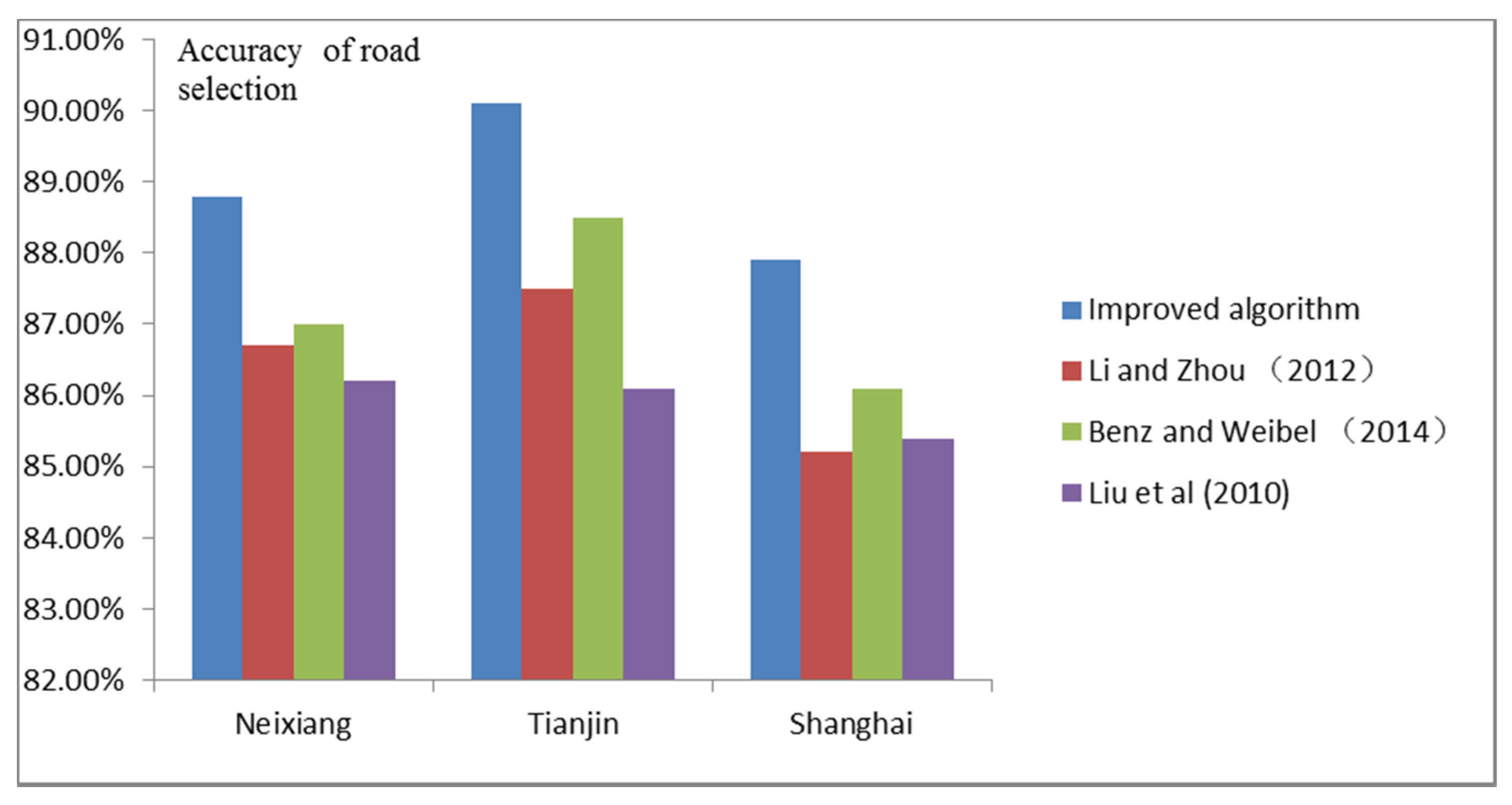
The hybrid road selection methods based on references [16,17,18] were selected and compared with the improved method proposed in this paper. The road selection accuracy of different methods can be determined by comparing results for existing maps with road networks obtained by different methods. In order to verify the reliability of the results, Neixiang, Tianjin, and Shanghai case data at a 1:50,000 scale were used to conduct comparison tests. The accuracy of road selection using different methods is depicted in Figure 15. As can be seen in Figure 15, the improved method performs better than the other three methods in different study areas.
Nevertheless, there are limitations to this study. The computational runtime of the improved method is a little longer than that of the stroke-based method or the mesh density-based method. However, all of these methods only take several minutes. In the future, we plan to advance the generation efficiency of weighted Voronoi diagrams in order to compensate for this. In addition, road selection requires a combination with other background information, such as the distribution of residents.
5. Conclusions
We proposed a new dual representation mode for road selection that combined an improved stroke generation algorithm with weighted Voronoi diagrams. This method designs overall connection rules by introducing an OLS model and improves connection strategies by implementing road importance. To overcome the limitations of existing partition methods, the proposed algorithm utilizes a weighted Voronoi diagram that includes road importance as a weighting parameter to partition road networks. Specifically, stroke importance and density threshold were both used as constraint indicators to control road selection. Combining global and local viewpoints, stroke importance was obtained using four evaluation indicators: stroke closeness, betweenness, length and degree. The density threshold was calculated using the smallest visible object based on a natural principle method.
Several case studies were conducted using the proposed method, and the accuracy of stroke generation and road selection were measured. Experimental results indicated that the proposed method maintained the overall characteristics of a road network, with spatial distribution information for a selection result varying only slightly compared with the original road network. Furthermore, the improved stroke generation algorithm also exhibited global and unique results. The proposed method achieved higher accuracy for road selection when compared with other methods, based solely on a linear or areal approach, as well as some hybrid methods. In addition, the proposed method has promising applicability because it does not rely on road attributes.
Acknowledgments
This work is based upon work supported by Natural Science Foundation of China (No. 41371375), Natural Science Foundation of Beijing (8132018), as well as by the International Exchange and Joint Training Program of the Graduate School of Capital Normal University. We also thank the anonymous referees for their helpful suggestions.
Author Contributions
Jianchen Zhang performed the data analyses of the study and wrote the manuscript. Yanhui Wang contributed significantly to the conception of the study. Wenji Zhao helped perform the analysis and contributed to constructive discussions. All authors read and approved the final manuscript.
Conflicts of Interest
The authors declare that they have no conflict of interest.
References
- Zhou, Q.; Li, Z. How Many Samples are Needed? An Investigation of Binary Logistic Regression for Selective Omission in a Road Network. Cartogr. Geogr. Inf. Sci. 2016, 43, 405–416. [Google Scholar] [CrossRef]
- Suba, R.; Meijers, M.; Oosterom, P. Continuous Road Network Generalization throughout All Scales. ISPRS Int. J. Geo-Inf. 2016, 5, 145. [Google Scholar] [CrossRef]
- Dijk, T.C.; Haunert, J.H.; Oehrlein, J. Location-dependent generalization of road networks based on equivalent destinations. Comput. Gr. Forum 2016, 35, 451–460. [Google Scholar] [CrossRef]
- Thomson, R.; Brook, R. Generalisation of Geographical Networks. In Generalisation Geographic Information: Cartographic Modelling and Applications; Elsevier: Amsterdam, The Netherlands, 2007; pp. 255–268. [Google Scholar]
- Thomson, R.C.; Richardson, D.E. The Good Continuation Principle of Perceptual Organisation Applied to the Generalisation of Road Networks. In Proceedings of the 19th International Cartographic Conference, 11th General Assembly of ICA, Ottawa, ON, Canada, 14–21 August 1999; pp. 1215–1223. [Google Scholar]
- Jiang, B.; Claramunt, C. A Structural Approach to the Model Generalisation of an Urban Street Network. GeoInformatic 2004, 8, 157–171. [Google Scholar] [CrossRef]
- Touya, G. A Road Network Selection Process Based on Data Enrichment and Structure Detection. Trans. GIS 2010, 14, 595–614. [Google Scholar] [CrossRef]
- Xu, Z.; Liu, C.; Zhang, H. Road Selection Based on Evaluation of Stroke Network Functionality. Acta Geod. Cartogr. Sin. 2012, 41, 769–776. [Google Scholar]
- Yang, B.; Luan, X.; Li, Q. Generating Hierarchical Strokes from Urban Street Networks Based on Spatial Pattern Recognition. Int. J. Geogr. Inf. Sci. 2011, 25, 2025–2050. [Google Scholar] [CrossRef]
- Zhou, Q.; Li, Z. A Comparative Study of Various Strategies to Concatenate Road Segments into Strokes for Map Generalization. Int. J. Geogr. Inf. Sci. 2012, 26, 691–715. [Google Scholar] [CrossRef]
- Hh, H.; Qian, H.; Liu, H.; Wang, X.; Hu, H. Road Network Selection Based on Road Hierarchical Structure Control. Acta Geod. Cartogr. Sin. 2015, 44, 453–461. [Google Scholar]
- Hu, Y.; Chen, J.; Li, Z.; Zhao, R. Selective Omission of Road Features Based on Mesh Density for Digital Map Generalization. Acta Geod. Cartogr. Sin. 2007, 36, 351–357. [Google Scholar]
- Wanning, P.; Muller, J.C. A Dynamic Decision Tree Structure Supporting Urban Road Network Automated Generalization. Cartogr. J. 1996, 33, 5–10. [Google Scholar]
- Tian, J.; Ma, M.; Yang, X.C. An Approach to Constraint Based Urban Street Network Automated Generalization. Sci. Surv. Mapp. 2008, 33, 158–160. [Google Scholar]
- Chen, J.; Hu, Y.; Li, Z.; Zhao, R.; Meng, L. Selective Omission of Road Features Based on Mesh Density for Automatic Map Generalization. Int. J. Geogr. Inf. Sci. 2009, 23, 1013–1032. [Google Scholar] [CrossRef]
- Li, Z.; Zhou, Q. Integration of Linear and Areal Hierarchies for Continuous Multiscale Representation of Road Networks. Int. J. Geogr. Inf. Sci. 2012, 26, 855–880. [Google Scholar] [CrossRef]
- Benz, A.; Weibel, R. Road network selection for medium scales using an extended stroke-mesh combination algorithm. Cartogr. Geogr. Inf. Sci. 2014, 41, 323–339. [Google Scholar] [CrossRef]
- Liu, X.; Zhan, F.; Ai, T. Road Selection Based on Voronoi Diagrams and “Strokes” in Map Generalization. Int. J. Appl. Earth Obs. Geoinf. 2010, 12, 194–202. [Google Scholar] [CrossRef]
- Tian, J.; Song, Z.H.; Ai, T.H. Grid Pattern Extraction in Road Networks with Graph. Geomat. Inf. Sci. Wuhan Univ. 2012, 37, 724–727. [Google Scholar]
- Chen, B.; Wu, F.; Qian, H.Z. Study on Road Networks Auto_selection Algorithms. J. Image Gr. 2008, 13, 2388–2393. [Google Scholar]
- Borruso, G. Network Density and the Delimitation of Urban Areas. Trans. GIS 2003, 7, 177–191. [Google Scholar] [CrossRef]
- Li, S.; Zhou, Q.; Wang, L. Road Construction and Landscape Fragmentation in China. J. Geogr. Sci. 2004, 15, 123–128. [Google Scholar] [CrossRef]
- Liu, X.; Ai, T.; Liu, Y. Road Density Analysis Based on Skeleton Partitioning for Road Generalization. Geo-Spat. Inf. Sci. 2009, 12, 110–116. [Google Scholar] [CrossRef]
- Tian, J.; Ren, C.; Wang, Y.; Xiong, F.; Lei, Y. Improvement of Self-Best-Fit Strategy for Stroke Building. Geomat. Inf. Sci. Wuhan Univ. 2015, 40, 1209–1214. [Google Scholar]
- Jiang, B.; Zhao, S.; Yin, J. Self-organized natural roads for predicting traffic flow: A sensitivity study. J. Stat. Mech. 2008. [Google Scholar] [CrossRef]
- Tian, J.; He, Q.S.; Yan, F. Formalization and New Algorithm of Stroke Generation in Road Networks. Geomat. Inf. Sci. Wuhan Univ. 2014, 39, 556–560. [Google Scholar]
- Diakoulaki, D.; Mavritas, G.; Papayannakis, L. Determining Objective Weights in Multiple Criteria Problems: The CRITIC Method. Comput. Oper. Res. 1995, 22, 763–770. [Google Scholar] [CrossRef]
- Ge, R. The Design and Implementation of Add-in Generating Voronoi Diagram with Multiple Weighted Generators Based on ArcObjects; Resources Environment and Earth Science of Yunnan University: Kunming, China, 2015. [Google Scholar]
- Li, Z.L.; Openshaw, S. Algorithm for automated line generalization based on a natural principle of objective generalization. Int. J. Geogr. Inf. Syst. 1992, 6, 373–389. [Google Scholar] [CrossRef]
- Li, Z.L.; Openshaw, S. A natural principle for objective generalization of digital map data. Cartogr. Geogr. Inf. Syst. 1993, 20, 19–29. [Google Scholar] [CrossRef]
- Müller, J. Optimum point density and compaction rates for the representation of graphic lines. Proc. AutoCarto 1987, 8, 221–230. [Google Scholar]
- Töpfer, F.; Pillewizer, W. The Principles of Selection: a Means of Cartographic Generalization. Cartogr. J. 1966, 3, 10–16. [Google Scholar] [CrossRef]
- Kruskal, J. On the Shortest Spanning Subtree of a Graph and the Travelling Salesman Problem. Am. Math. Soc. 1956, 7, 48–50. [Google Scholar] [CrossRef]
Figure 1.
Calculation of road deflection angle.

Figure 2.
Calculation of declination rate.

Figure 3.
Calculation flowchart for stroke connection rules.

Figure 4.
Diagrammatical rules for road connections.

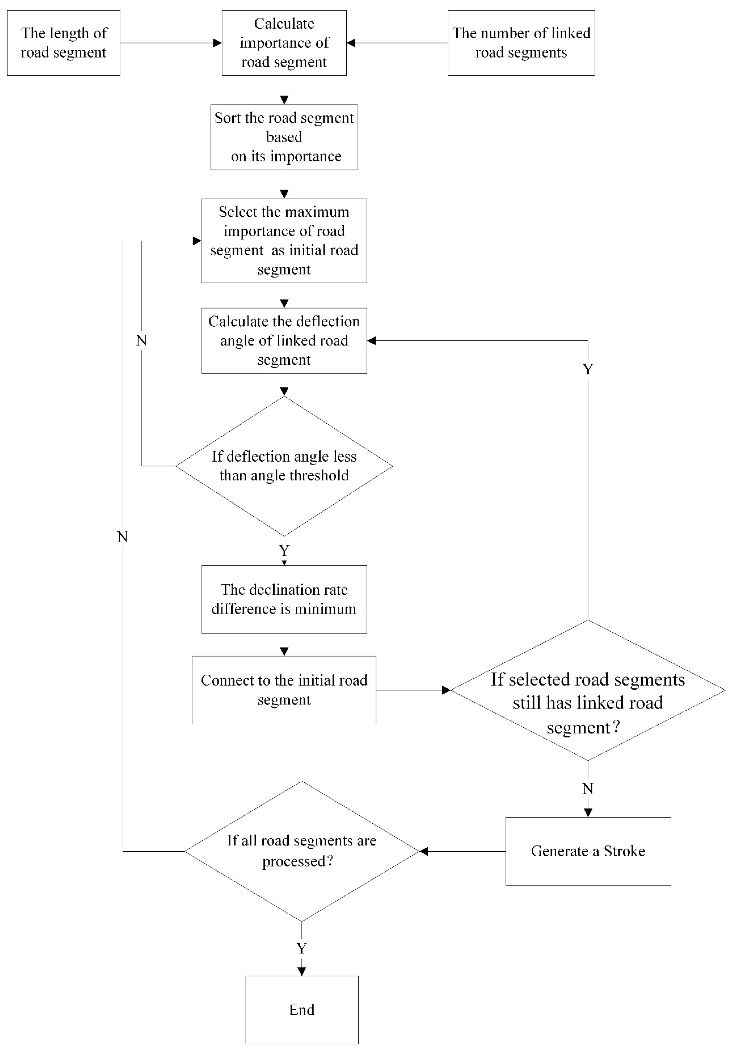
Figure 5.
A flowchart for the improved stroke algorithm.

Figure 6.
Partition results for the ordinary and weighted Voronoi diagrams: (a) weighted Voronoi diagram; (b) ordinary Voronoi diagram.
Figure 6.
Partition results for the ordinary and weighted Voronoi diagrams: (a) weighted Voronoi diagram; (b) ordinary Voronoi diagram.
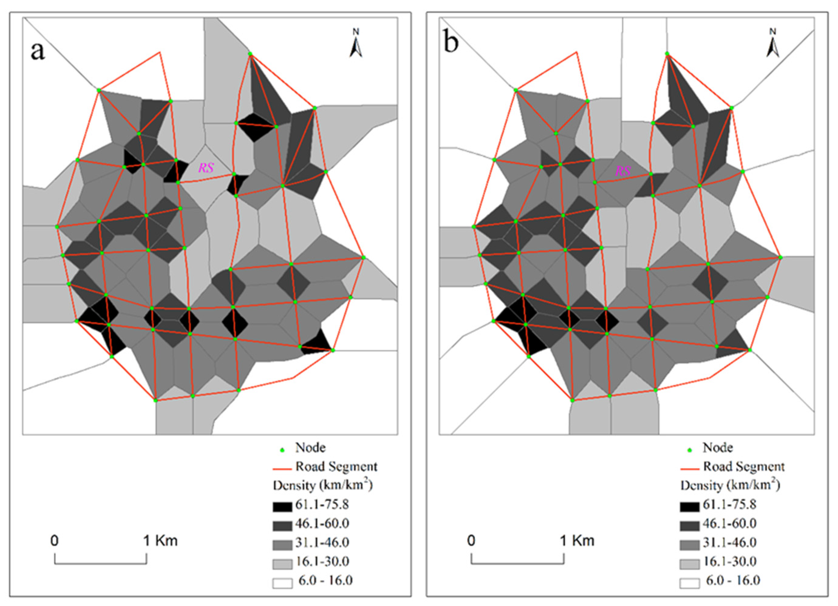
Figure 7.
A flowchart for the road selection process.

Figure 8.
The original road network data.

Figure 9.
The results of stroke generation.

Figure 10.
Local contrast for stroke generation.
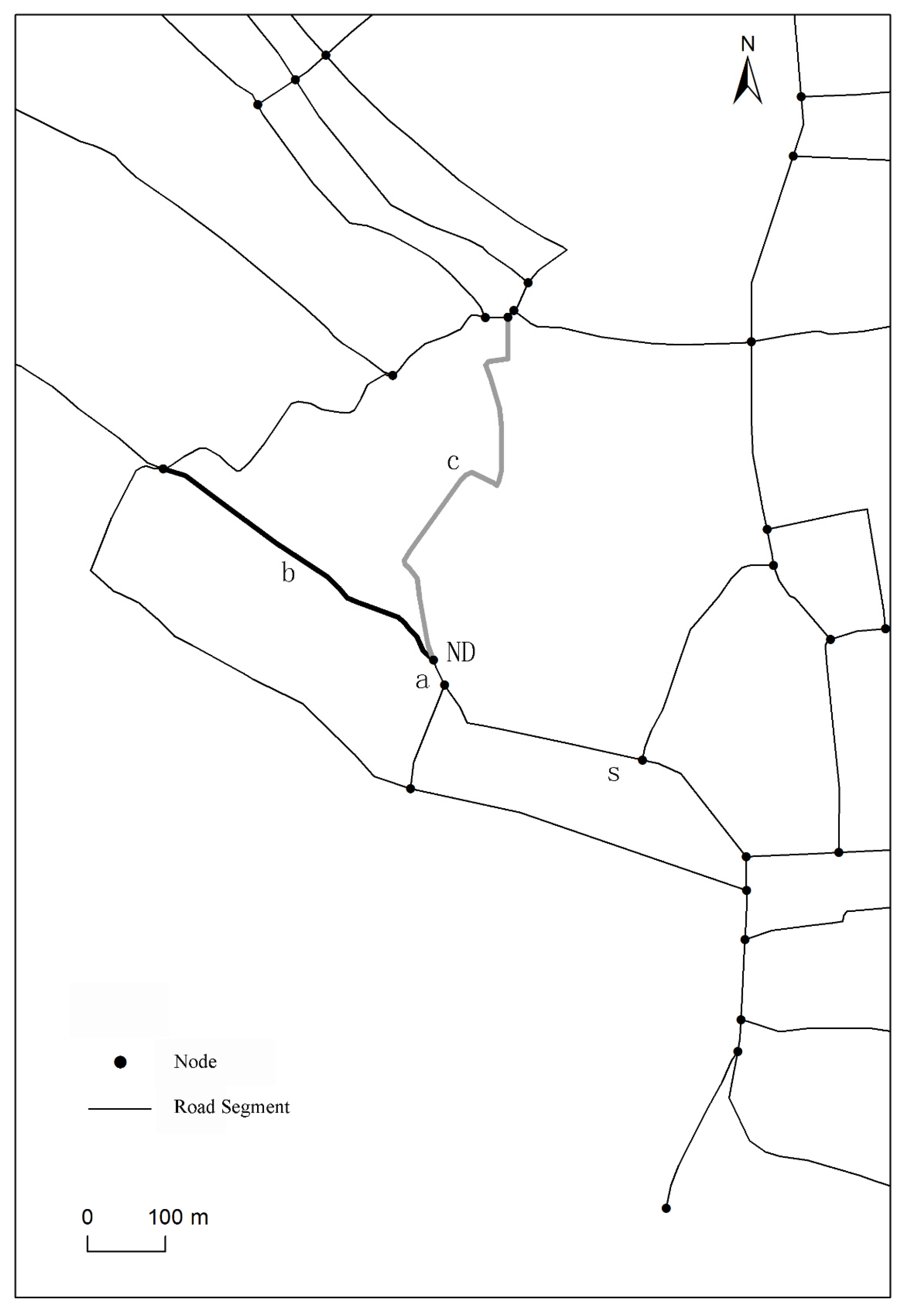
Figure 11.
Global efficiency based on different stroke generation methods.

Figure 12.
A comparison of selection processes for the weighted Voronoi method and the mesh method; (a) a schematic road network with areal road segments; (b) selection results based on the mesh method for an areal road pattern; (c) selection results based on the weighted Voronoi diagram for an areal road pattern; (d) a schematic road network with hybrid road segments; (e) selection results based on the mesh method for a hybrid road pattern; (f) selection results based on the weighted Voronoi diagram method for a hybrid road pattern.
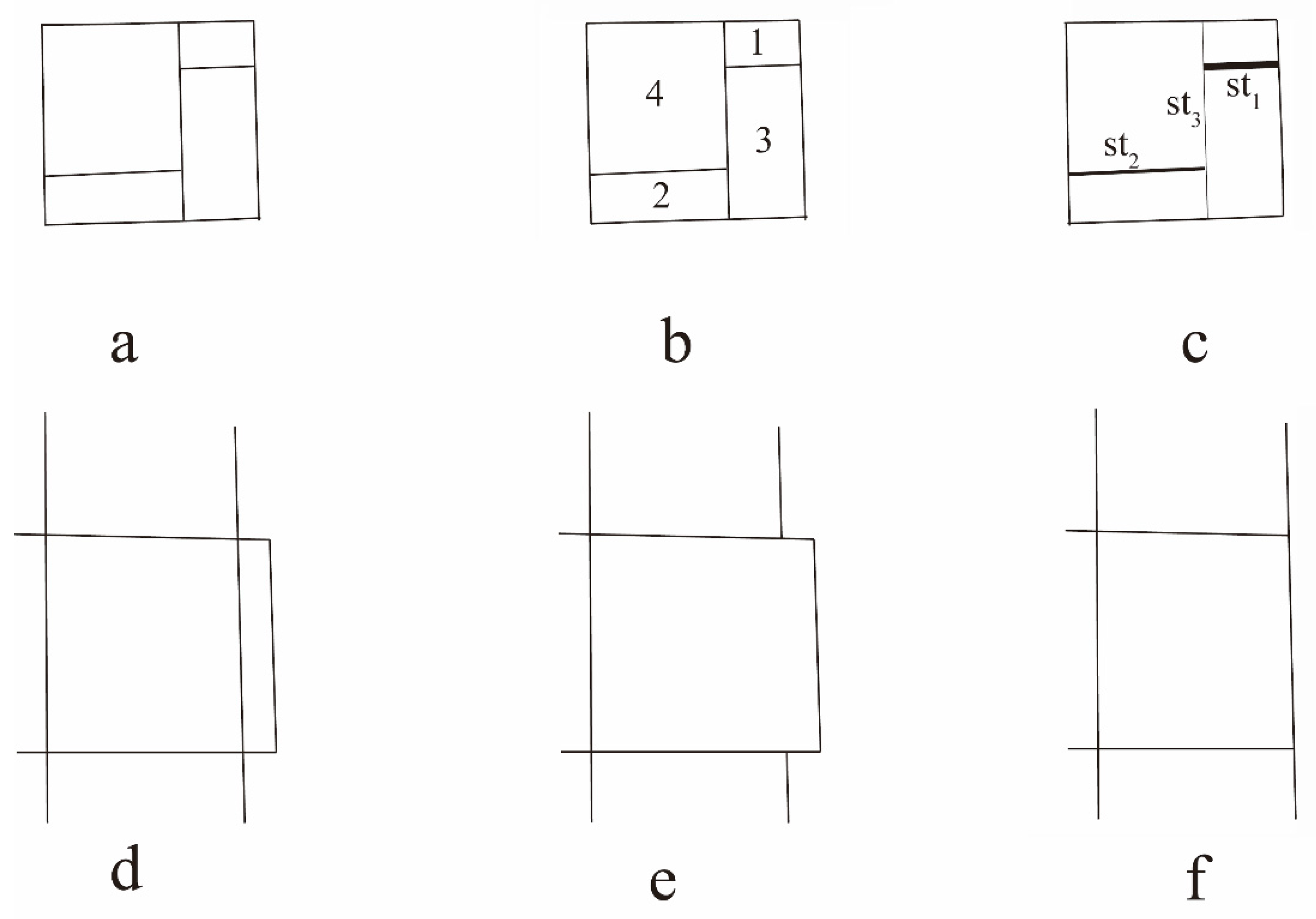
Figure 13.
A local comparison of different road selection methods.

Figure 14.
The results of road selection and deletion.

Figure 15.
Accuracy of different road selection methods.


Table 1.
Pseudo-code for the stroke generation algorithm.
| Set S = Sort (Isegment); //Sort the importance of road segment If (S! == NULL) { Bool IsSelected = False; Initial segment = max (S); //Select road segment that has the maximum importance as the initial road segment Initial segment_IsSelected = True; //Set the property of initial road segment as True. IsLinked (Initial segment); Update S (); } IsLinked (Initial segment) //Judge whether road segment connects { Get the neighbor segments’ number of Initial segment; //Get the linked road segment of initial segment If (k = 0) Set ST = ST + Initial segment; //Build a new Stroke For neighbor segment = 1 to k //k is the number of linked road segments Calculate the deflection angle; //Calculate deflection angle If (deflection angle <= θ) Δ m = |msegment - mInitial segment|; Else Return; Linked segment = min (Δ m) segment; Linked segment_IsSelected = True; //Mark the connected road segment Set Initial segment = Linked segment; } Update S () //Update the road network { Set S_selected = Initial segment; S = S - S_selected; } |
Table 2.
Parameter explanation and calculation of stroke importance.
| Stroke Evaluation Indicator | Explanation | Calculated Equation |
|---|---|---|
| Stroke Length (L) | The total length of road segments formed by stroke | , is the length of kth road segment of ith Stroke. |
| Stroke Degree (D) | The total number of road segment formed by stroke | If road segment is part of Stroke then = 1, or = 0. |
| Stroke Betweenness (B) | The probability of a stroke lying in the other strokes | , (j ≠ k; j, k ≠ i), N is the number of node; is the number of shortest paths between node j and node k; is the number of shortest paths between node j and node k that contains node i. |
| Stroke Closeness (C) | The minimal connection number of a stroke to other stroke, reflecting the probability of a stroke being close to the another stroke | , represents the shortest distance of Stroke and Stroke . |
Table 3.
Statistical results for different stroke generation methods.
| Method | Number of Correct Types | Number of False Types | Sample Size | Accuracy Rate (%) |
|---|---|---|---|---|
| Improved algorithm | 92/178 | 8/22 | 100/200 | 92/90 |
| Every-best-fit | 83/158 | 17/42 | 100/200 | 83/79 |
| Self-best-fit | 79/150 | 21/50 | 100/200 | 79/75 |
| Self-fit | 72/138 | 28/62 | 100/200 | 72/69 |
| Sum | 326/624 | 74/176 | 400/800 | 82/78 |
The samples size is 100 and 200 before and after the notation “/”, respectively.
Table 4.
Chi-square test results.
| Sample Size | Chi-Square | Degrees of Freedom | Significance |
|---|---|---|---|
| 100 | 15.2 | 3 | 13.8 > 7.82, Yes |
| 200 | 24.7 | 3 | 24.7 > 7.82, Yes |
Table 5.
The results of the Marascuilo procedure.
| Methods | Absolute Difference | Critical Range | Significance |
|---|---|---|---|
| Improved algorithm and Every-best-fit | 0.09/0.11 | 0.065/0.051 | Yes/Yes |
| Improved algorithm and Self-best-fit | 0.13/0.15 | 0.078/0.059 | Yes/Yes |
| Improved algorithm and Self-fit | 0.20/0.21 | 0.087/0.063 | Yes/Yes |
The sample size is 100 and 200 before and after the notation “/”, respectively.
Table 6.
Statistics results of different stroke generation methods.
| Study Area | Stroke Generation Method | Length of Selected Road Segment (Km) | Length of Identical Strokes with Existing Map (Km) | Length of Identical Road Segments/Existing Map (%) | Length of Identical Road Segments/Automated Algorithm Result (%) | Accuracy of Road Selection (%) |
|---|---|---|---|---|---|---|
| Neixiang County (The length of existing map is 72.3 (Km)) | Improved Method | 74.8 | 65.4 | 90.1 | 87.4 | 88.8 |
| Every-best-fit | 76.1 | 62.2 | 86.0 | 81.8 | 83.9 | |
| Self-best-fit | 77.4 | 60.8 | 84.1 | 78.5 | 81.3 | |
| Self-fit | 79.2 | 58.0 | 80.2 | 73.2 | 76.7 | |
| Tianjin City (The length of existing map is 108.7 (Km)) | Improved Method | 111.4 | 96.4 | 88.7 | 86.5 | 87.6 |
| Every-best-fit | 113.7 | 89.6 | 82.4 | 78.8 | 80.6 | |
| Self-best-fit | 114.2 | 86.7 | 79.8 | 75.9 | 77.9 | |
| Self-fit | 110.5 | 93.0 | 85.6 | 84.2 | 84.9 | |
| Shanghai City (The length of existing map is 214.5 (Km)) | Improved Method | 217.7 | 185.5 | 86.5 | 85.2 | 85.9 |
| Every-best-fit | 216.3 | 174.1 | 81.2 | 80.5 | 80.9 | |
| Self-best-fit | 220.2 | 181.7 | 84.7 | 82.5 | 83.6 | |
| Self-fit | 218.4 | 171.2 | 79.8 | 78.4 | 79.6 |
Table 7.
Statistical results for different road selection methods.
| Road Selection Method | Length of Selected Road Segment (The length of Selected Road Segment by Manual Selection is 72.3 (Km)) | Length of Identical Strokes with Manual Results | Length of Identical Road Segments/Manual Result (%) | Number of Identical Road Segments/Automated Algorithm Result (%) | Accuracy of Road Selection (%) |
|---|---|---|---|---|---|
| Stroke-Based Method | 78.9 | 60.9 | 84.2 | 77.2 | 80.7 |
| Mesh Density-Based Method | 76.7 | 61.2 | 80.2 | 79.8 | 78.5 |
| Improved Method | 74.8 | 65.4 | 90.1 | 87.4 | 88.8 |
© 2017 by the authors. Licensee MDPI, Basel, Switzerland. This article is an open access article distributed under the terms and conditions of the Creative Commons Attribution (CC BY) license (http://creativecommons.org/licenses/by/4.0/).
Share and Cite
MDPI and ACS Style
Zhang, J.; Wang, Y.; Zhao, W. An Improved Hybrid Method for Enhanced Road Feature Selection in Map Generalization. ISPRS Int. J. Geo-Inf. 2017, 6, 196. https://doi.org/10.3390/ijgi6070196
AMA Style
Zhang J, Wang Y, Zhao W. An Improved Hybrid Method for Enhanced Road Feature Selection in Map Generalization. ISPRS International Journal of Geo-Information. 2017; 6(7):196. https://doi.org/10.3390/ijgi6070196
Chicago/Turabian StyleZhang, Jianchen, Yanhui Wang, and Wenji Zhao. 2017. "An Improved Hybrid Method for Enhanced Road Feature Selection in Map Generalization" ISPRS International Journal of Geo-Information 6, no. 7: 196. https://doi.org/10.3390/ijgi6070196
Note that from the first issue of 2016, this journal uses article numbers instead of page numbers. See further details here.