Topographic Correction to Landsat Imagery through Slope Classification by Applying the SCS + C Method in Mountainous Forest Areas

Abstract

The aim of the topographic normalization of remotely sensed imagery is to reduce reflectance variability caused by steep terrain and thus improve further processing of images. A process of topographic correction was applied to Landsat imagery in a mountainous forest area in the south of Mexico. The method used was the Sun Canopy Sensor + C correction (SCS + C) where the C parameter was differently determined according to a classification of the topographic slopes of the studied area in nine classes for each band, instead of using a single C parameter for each band. A comparative, visual, and numerical analysis of the normalized reflectance was performed based on the corrected images. The results showed that the correction by slope classification improves the elimination of the effect of shadows and relief, especially in steep slope areas, modifying the normalized reflectance values according to the combination of slope, aspect, and solar geometry, obtaining reflectance values more suitable than the correction by non-slope classification. The application of the proposed method can be generalized, improving its performance in forest mountainous areas.

1. Introduction

1.1. Background

The determination of the reflectance value of the surface by removing topographic effects is an important task in remote sensing studies [1]. However, the ability to provide reliable information through satellite imagery is constrained by the effects that changes in slope and terrain orientation angles (aspect) in combination to the solar geometry (zenithal and azimuthal angles) at the time of the image acquisition cause on the spectral direct and diffuse irradiance [2].

This occurs especially in mountainous areas where slope surfaces directly oriented to sun rays receive more light and consequently appear brighter in images than those surfaces that are not receiving the sunlight directly [3].

This difference of illumination and variation of the proportion of light reflected from the ground to the sensor is due to the diversification of the sun-target-sensor geometry, which, in turn, depends on the topographic relief [4]. This effect causes an additional alteration of the radiometric data on pixels with the same land cover, similar structure, and biophysical properties [5,6], which can lead us to errors in subsequent processes and reduce the quality of the results [7,8,9].

Topographic correction methods applied in remote sensing comprise cosine, Minnaert, Civco two-stages, statistical-empirical, and Factor C, which have been extensively studied [4,5,6,10,11,12,13,14,15,16].

The application of models based on geometry of the sun-canopy-sensor (SCS) is more appropriate in forest areas than other ground-based methods because SCS preserves the geotropic nature of the trees (growth normal to the geoid) [17].

The photometric-empirical topographic standardization models, such as Minnaert correction [10] or C-correction [4], applies semi-empirical methods, which consist of a photometric function modified by an empirical parameter obtained from the relationship between the spectral data and the illumination conditions [2].

The SCS + C topographic correction method considers a global correction C-parameter determined for each band of the scene. Teillet et al. [4] state that the C-parameter exerts a moderating influence on cosine correction method by increasing the denominator and reduce overcorrection of dimly lit pixels. This adjustment has shown that the spectral characteristics of data are retained and improves the classification accuracy in mountainous areas [18,19].

Some studies have emphasized the calculation of empirical parameters, Civco [11] focused on the aspect considering samples of an equal number of pixels, but distinguishing northern and southern slopes. Smith et al. [10], Ekstrand [20], and Blesius and Weirich [21] made a selection of pixels of the same land cover under different topographic conditions.

Other studies have considered a random sampling of the entire image or a subset of pixels; Teillet et al. [4] estimated the parameters for five different types of forest; Colby [22] estimated a global parameter considering an entire Landsat TM image and a local parameter from a subset of pixels in forest area, while Bishop and Colby [23] conducted a comparison of empirical parameters calculated globally, locally, and specifically for three broad land cover types using Spot imagery. Reese and Olson [2] made random samples with stratification on north and south aspects and stratification by the cosine of the solar incidence angle, i.

Due to the wide ranges of elevations and slopes, the mountainous regions have particular effects in their interaction with radiation [24]. The quantity of radiation reflected by targets depends on the specific class of reflection in multiple directions that describe the bidirectional reflectance function BDRF [25], but, according to Ekstrand [20], also depends on whether the geometric structure of the forest type changes with the slope.

Kimes and Kirchner [26] recognized that the effects of the slope and aspect on target radiance for all wavelengths ranging in mountain areas are significant for all topographic surfaces, from the radiance that is highly absorbed to the radiance that is highly reflected.

Measurements of topographic effects have demonstrated that different types of vegetation respond differently to direction and illumination effects [3,13,27,28,29]. However, it is not always possible to have a suitable land cover map close enough to the date of analysis, appropriate according to the study scale, and showing, in detail, the classes of interest. On the other hand, to have a digital elevation model (DEM) and a derived slope map is relatively easy; thus, it would also be easier to develop the proposed method seeking to improve the topographical correction without relying on a land cover map.

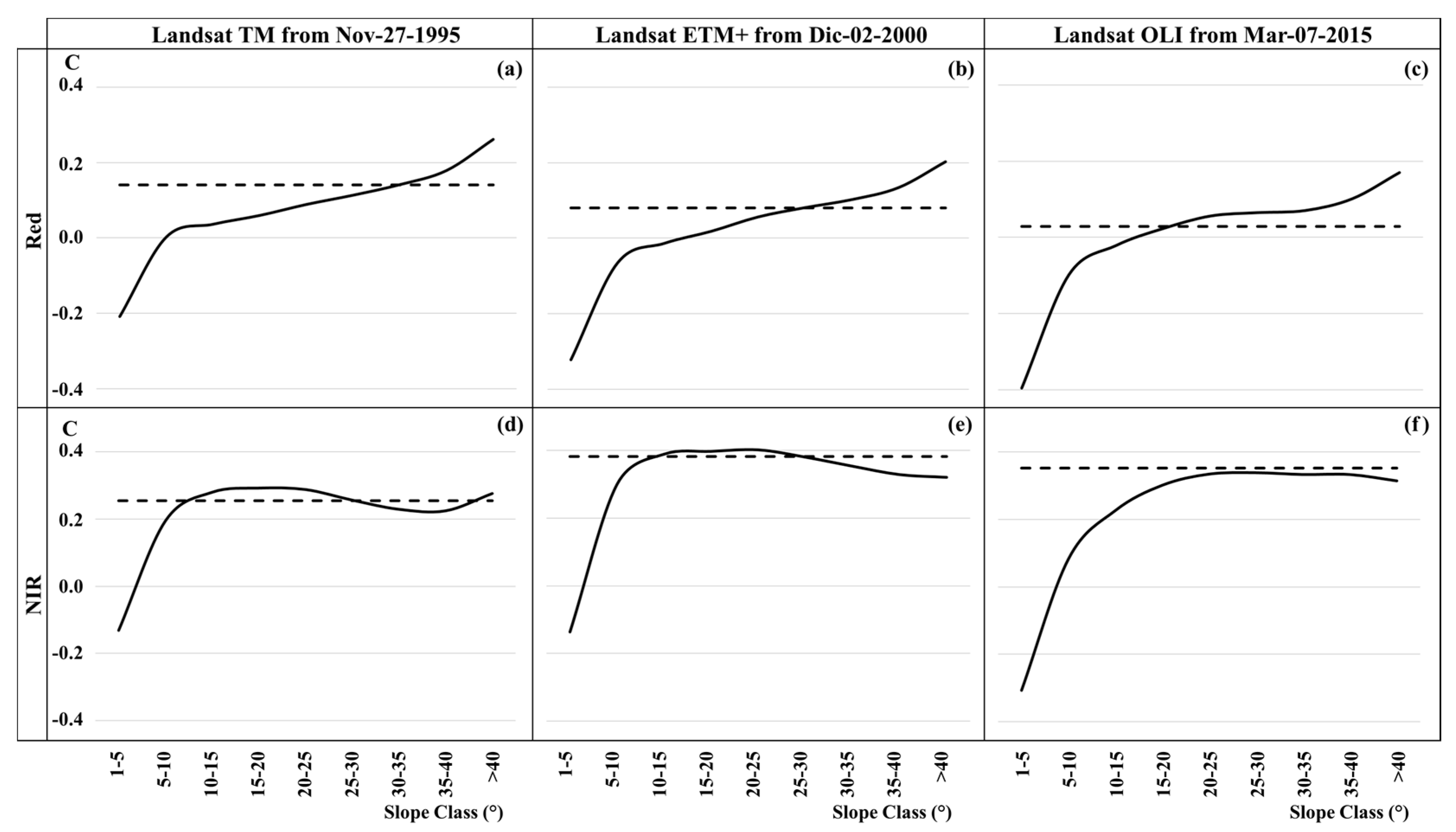
1.2. The C Parameter

According to this background, the high, steep changes and land coverage variations present in mountainous regions cause effects on illumination and reflected radiation, a fact that theoretically directly affects the determination of the value of the correction C parameter used in the topographic correction of empirical correction models. That is, the application of a unique global correction C parameter may not produce an accurate topographic correction for the whole scene because of slope variation.

The aim of this study is to assess, qualitatively and quantitatively, the results of topographic correction of Landsat images through the SCS + C method, by non-slope classification (N-SC) and by slope classification (SC). To achieve the proposed aim, a comparative analysis between reflectance images normalized by the standard SCS + C topographic correction method (with a single global C parameter) and reflectance images normalized by the same approach but where nine C parameters were determined by applying a classification based on the slopes of the studied zone.

For this work, Dinamica EGO software [30,31,32] was used to develop the described models and processes.

2. Materials and Methods

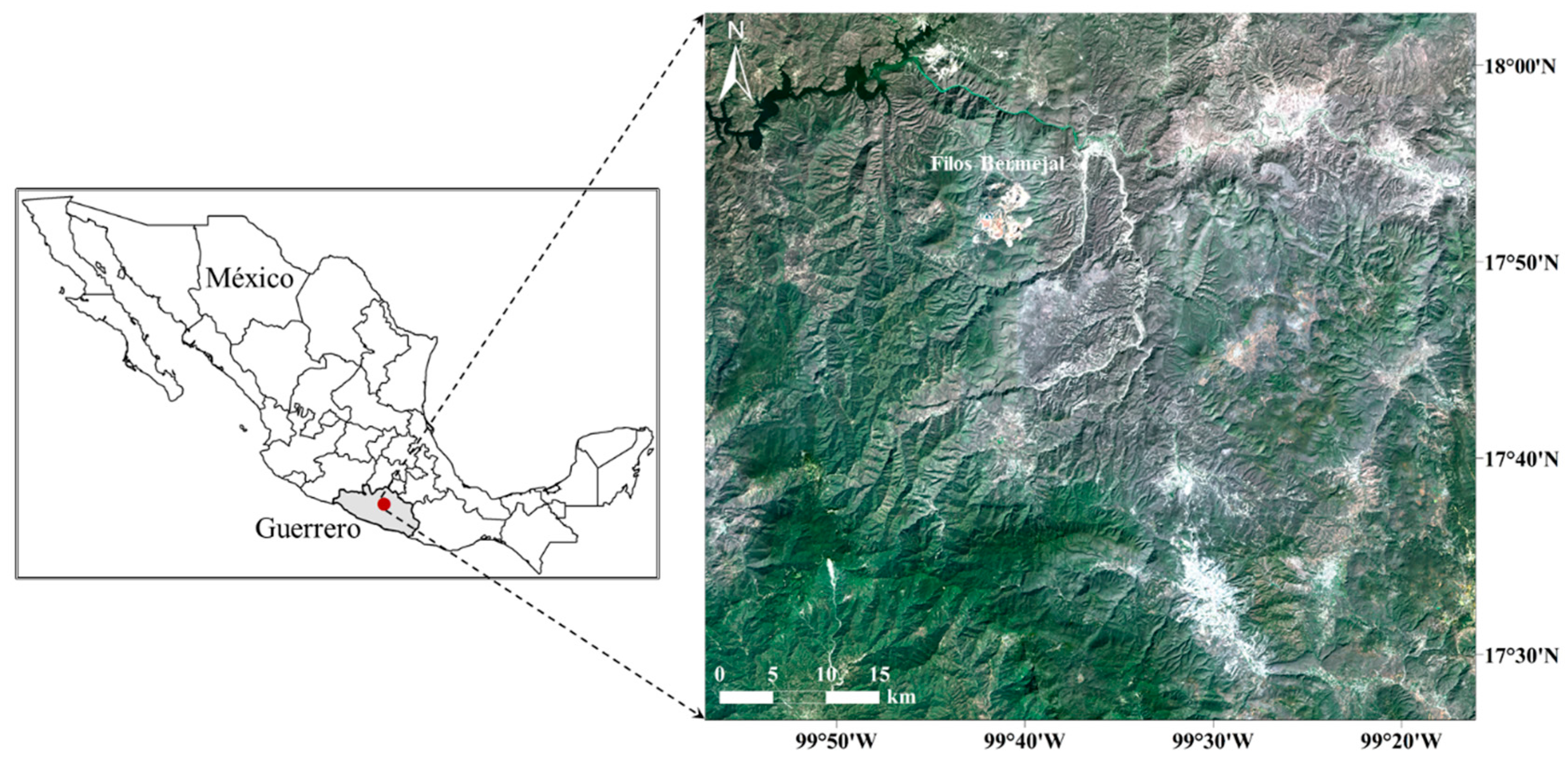
2.1. Study Area and Dataset

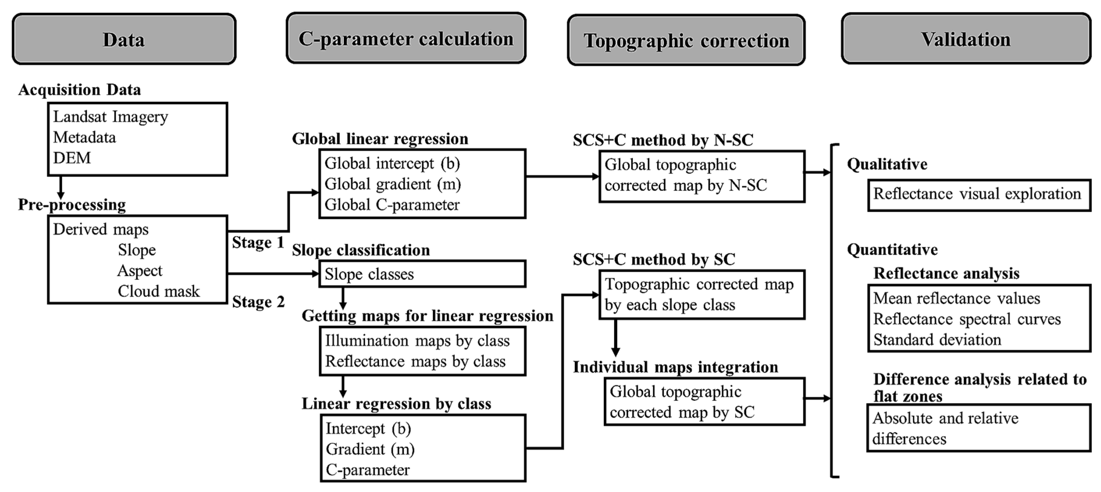
The studied area consists of a group of basins in the central region of the Guerrero state in Mexico, around the largest gold mine in Latin America, “Filos-Bermejal” [33], that covers nearly 4000 km² of mountain terrain with altitudes from 580 to 2840 m above the sea level, where slopes greater than 40° are present (Figure 1).

The land cover distribution of the zone is 45% of oak, pine, and mesophyll forest, 36% of deciduous forest, and 19% of grassland, agricultural, bare soil, water, and urban area [34,35].

The vegetation types refer to the different groups that are presented in the zone and that are part of the large of vegetation ecological information, floristics, and physiognomy. The types of vegetation included as land cover are as follows [36]: Oak, pine, and mesophyll forest, including secondary bushy vegetation that corresponds to areas where the particular ecological original conditions of the community have been altered and where each plant community has a group of minor species that cover the altered space.

The oak forest refers to arboreal, sub-arboreal, or occasional shrub communities integrated by multiple species of the genus Quercus that, in Mexico, except in very arid conditions, are located at altitudes from 300 to 2800 m. It is closely related to pine forests, forming mixed forests with species of both genera.

The pine forest includes arboreal, sub-arboreal, or occasionally shrub communities of northern (Holarctic) origin, mainly of milder and middle-cold weather regions with different degrees of humidity. Usually with minimal variation of species of conifers. Its development is a consequence of the climate and the soil of a region, which have not significantly influenced other factors for its establishment.

The mesophyll forest refers to plant communities characterized by the presence of dense to very dense tree vegetation, with epiphytes and ferns. These are located mainly in mountains, ravines, and sites that present favorable conditions of humidity and frequent fogs. In Mexico, these are located at altitudes between 600 m and 2800 m.

The deciduous forest refers to arboreal or sub-arboreal communities of tropical origin that grow in places with seasonal precipitation and where more than 75% of their plant components lose their leaves during the dry season of the year.

Three Landsat surface reflectance (SR) images (Path 26, Row 48, WRS-2) were used. This processed product is courtesy of the U.S. Geological Survey Earth Resources Observation and Science Center and is offered as Climate Data Records [37,38]. The images correspond to the dates and sensors: 11 November 1995 (L5-TM), 2 December 2000 (L7-ETM+), and 7 March 2015 (L8-OLI). The bands used were blue, green, red, near-infrared (NIR), shortwave infrared 1 (SWIR-1), and shortwave infrared 2 (SWIR-2), according to the official nomenclature [39].

The SR information is produced by the specialized software “Landsat Ecosystem Disturbance Adaptive Processing System” for Landsat 5-TM and L8SR for Landsat 8-OLI, developed by the Making Earth System Data Records for Use in Research Environments of the Goddard Space Flight Center of NASA and the University of Maryland [40].

The software applies the MODIS atmospheric correction routines. In addition to the Landsat data, the water vapor, ozone, geopotential height, aerosol optical thickness, and digital elevation data are presented to the radiative transfer model “Second Simulation of a Satellite Signal in the Solar Spectrum” (6S), to generate the top of atmosphere reflectance, SR, brightness temperature and cloud masks, cloud shadows, and adjacent clouds, land, and water.

The corresponding solar azimuth and zenith metadata angles used were 135.849° and 52.357° for L5-TM, 148.127° and 45.976° for L7-ETM+, and 127.516° and 34.995° for L8-OLI.

The land cover and vegetation map “Series I to IV” scale 1:250,000 were used, and a 30 m grid cell size DEM, which was generated from the vectorial data (contours) of the topographic maps, courtesy of the National Institute of Statistics and Geography of Mexico (INEGI), with a scale of 1:50,000 and 20 m for vertical accuracy.

2.2. Overview

The topographic corrections by SCS + C method were performed in two stages: first with a global C parameter determined by N-SC considering all pixels, and second with a set of nine C parameters determined by SC considering all those pixels with a slope greater than 0° (Figure 2).

The resulting corrected images were visually (qualitatively) explored and numerically (quantitatively) validated based on the normalized reflectance values obtained.

In concordance with previous works showing a close connection between the red band and the chlorophyll content and the near-infrared band linked to the density of vegetation [41,42], the resulting C parameters are presented and discussed for the red and near-infrared bands. Nevertheless, the reflectance values resulting from the topographic corrections are shown for each date, band, and slope class.

2.3. Correction C Parameter Calculation

The C parameter is determined by C = b/m, where b is the intercept and m is the gradient of the line obtained from the linear regression between the cosine of the solar incidence angle i (illumination) as the independent variable, and spectral data (reflectance) as the dependent variable.

The cosine of the incident solar angle (cos i), referred to as illumination [3,10,43], was calculated by

cos i = illumination = cos θp cos θi + sin θp sin θi cos (Φa − Φ0)

(1)

where θp is the terrain slope; θi is the solar zenith; Φa is the solar azimuth; Φ0 is the aspect.

The slope and aspect data were derived from the DEM, and the solar zenith and azimuth angles were obtained from the metadata files.

In the first stage, a global C(i) parameter was calculated (where i corresponds to the band), through a linear regression (illumination-reflectance) and considering all pixels, regardless of the slope variations.

In the second stage, due to the wide range of terrain slopes in the studied area, the C(i,j) parameter was defined for each band (i), considering a slope classification grouped into nine classes (j), with ranges of 5° each, for those pixels greater than 0°. In this case, for each slope class, a linear regression was performed just for the pixels considered in the range of the slope classes and excluding the rest.

Thus, for each band (i) and date image, first a single C(i) parameter value by N-SC was generated, and nine C(i,j) parameter values (one per class) by SC were later generated.

2.4. Topographic Correction

Soenen et al. [6] used the SCS + C method incorporating the C parameter to the SCS method, to characterize the diffuse atmospheric irradiance in a better way. The following equation expresses the model:

Ln = L (cos θp cos θi + C)/(cos i + C)

(2)

where Ln is the equivalent flat surface reflectance (normalized), L is the measured radiance in the remotely sensed data, and C is the semi-empirical parameter.

With the C(i,j) parameters obtained in each case (SC and N-SC), the SCS + C topographic correction method was applied, and normalized-reflectance images have been achieved for each band. In the case of topographic correction by SC, this process was performed for each class, and the resulting nine normalized-reflectance individual images (one per class) were later combined in a global final single image for each band.

2.5. Qualitative Validation

The visual exploration of images in remote sensing studies is a common method of assessing the quality of results [13,44]. The quantitative validation essentially consists of developing a visual comparative analysis between the reflectance images before topographic corrections, and images after the application of topographic correction either by N-SC or by SC; however, this is a subjective evaluation that can be inconvenient [45].

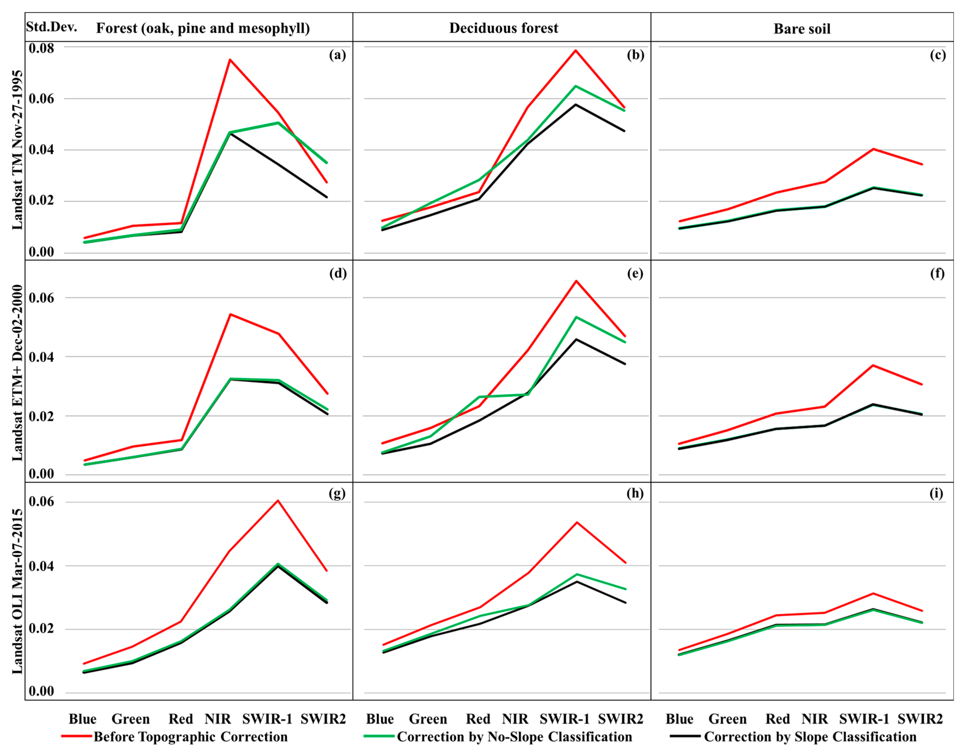
2.6. Quantitative Validation

To overcome the qualitative validation limitation, additional quantitative validations were performed: First, the effect of corrections over “oak, pine, and mesophyll forest,” “deciduous forest,” and “bare soil” land cover samples were analyzed, all of which had a broad range of slopes, enabling the identification of all slope classes used in the topographic correction process, and a wide variety of terrain orientations (aspect) were considered to have a broad range of shades as well.

For each date of the study, selected land cover, band, and slope class; the mean reflectance values before and after applying topographical corrections were obtained, and an analysis of standard deviation was performed.

In a second validation, it was considered that the topographic correction is based on the terrain slope, aspect, and geometry of the sun at the time of image acquisition; therefore, if the slope is null (flat terrain), the corrected reflectance values obtained by the SCS + C model equations are equal to the originally measured reflectance values.

Under this consideration for each date, land cover, band, and slope class, the absolute and relative differences between the mean normalized reflectance values of slope classes greater than 0° and mean normalized reflectance values of those pixels with a slope equal to 0° were calculated, considering these last pixels as topographically corrected, and an analysis of these differences was then performed.

To assess the relationship between the illumination (cos i) and reflectance values, an analysis through scatterplot graphs was conducted to the forest cover sample, before and after applying the topographic corrections (SC and N-SC), for each slope class.

3. Results and Discussion

3.1. C(i,j) Parameters

The variation of C(i,j) parameters obtained from the red and near-infrared bands considering SC can be seen (Figure 3), even becoming negative in the lower slope classes, unlike the global parameter determined by N-SC, the results of which are always positive.

It can be noted that the C(i,j) parameters by SC increase, according to the upper slopes, and critical values can be identified for those slopes where the values of both (N-SC and SC) C parameters are equal (at crossing lines).

It can also be noted that the patterns differ with the graphs obtained from the red band (Figure 3a–c) versus the graphs obtained for the infrared band (Figure 3d–f). For infrared graphs, the global C(i) parameters calculated by N-SC have less variation compared to those calculated by SC, which follows that the resulting reflectance values after N-SC and SC corrections are more similar to each other.

This difference between C parameters calculated by SC or N-SC undoubtedly produces different results in the normalized reflectance obtained by the topographic corrections, as shown below.

All C parameters (N-SC) and by slope classes (SC) resulting for each band, slope class, and date of study are included in Supplementary Materials Table S1.

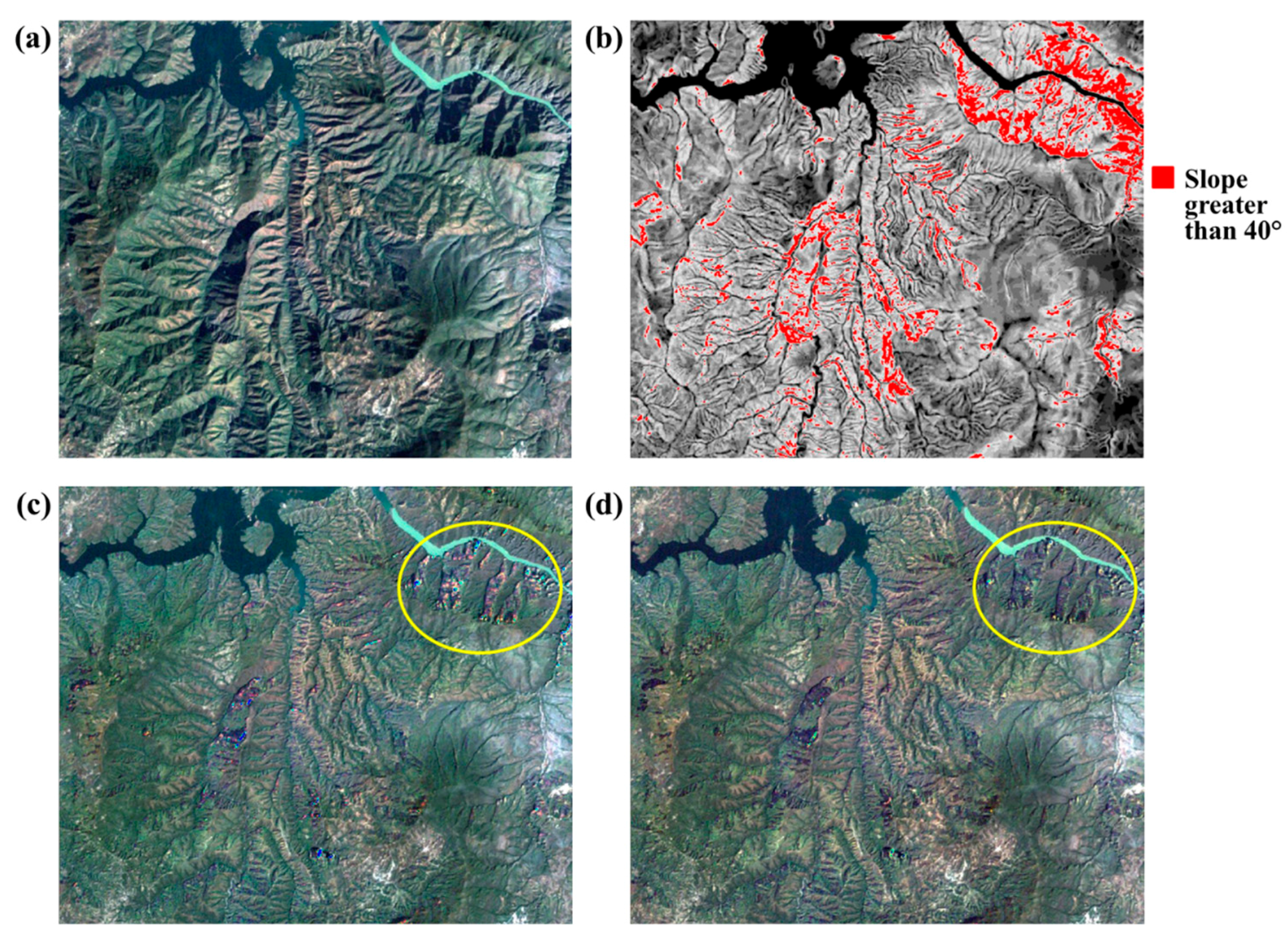
3.2. Qualitative Validation

The elimination of the shadows caused by relief and sun geometry at the time of image acquisition from the original image (Figure 4a) can be confirmed after the application of topographic correction processes (Figure 4c,d).

Visual results of both corrections are similar for areas with slopes that are not very steep; however, for areas that combine higher values of shadows and slope (greater than 40° as rounded in Figure 4c,d), it can be noted that the corrected image by SC (Figure 4d) shows a visual improvement compared to the corrected image by N-SC (Figure 4c).

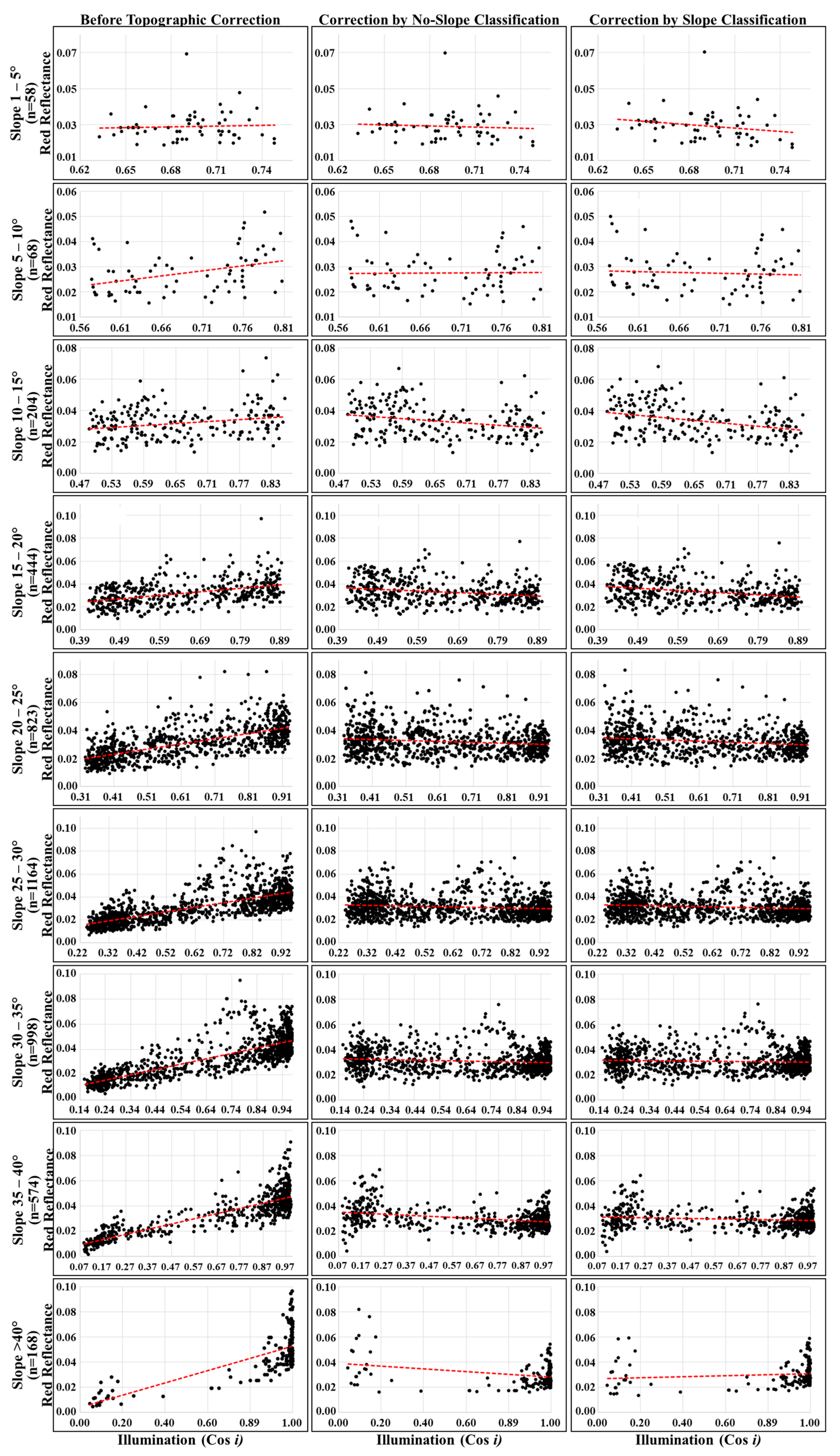
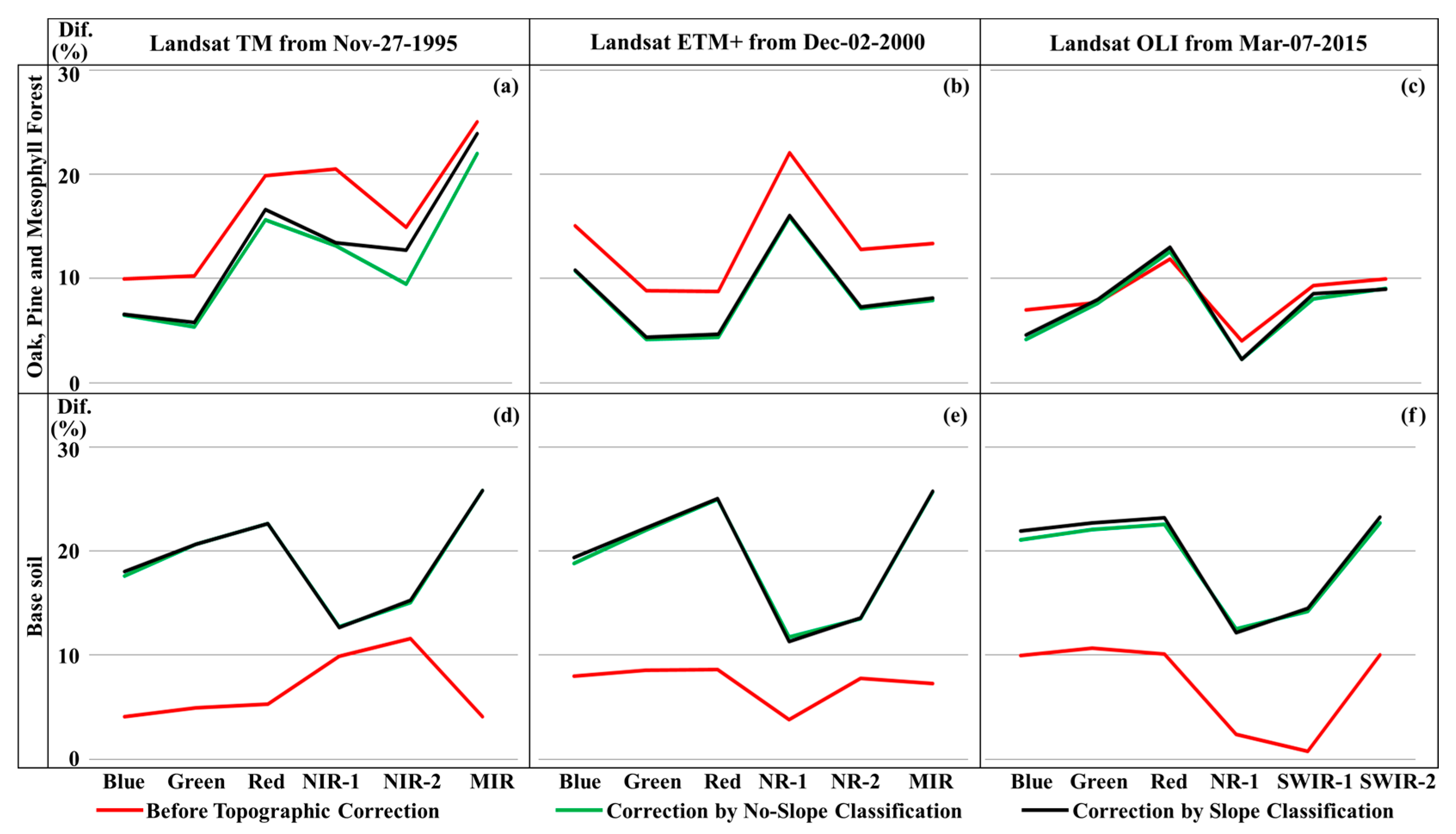
3.3. Quantitative Validation

Table 1. Standard deviation values before and after applying the topographic correction by N-SC and SC for each band and each slope class of oak, pine, and mesophyll forest. Image: Landsat OLI from 7 March 2015.

Slope Range (Degrees)	Blue			Green			Red
	Before Topographic Correction	After Topographic Correction		Before Topographic Correction	After Topographic Correction		Before Topographic Correction	After Topographic Correction
		NSC	SC		NSC	SC		NSC	SC
0	0.001900	0.001900	0.001900	0.001950	0.001950	0.001950	0.004250	0.004250	0.004250
0–5	0.013751	0.013327	0.012267	0.017763	0.017104	0.016473	0.024597	0.023910	0.023361
5–10	0.011086	0.010098	0.009958	0.017830	0.015883	0.015559	0.026320	0.023805	0.023460
10–15	0.007606	0.007311	0.006999	0.012198	0.012493	0.010869	0.019126	0.018849	0.018024
15–20	0.007812	0.007035	0.006688	0.012705	0.011657	0.010070	0.019961	0.018610	0.017696
20–25	0.008020	0.006162	0.006114	0.013389	0.009153	0.009129	0.020869	0.016726	0.016681
25–30	0.009193	0.005697	0.005632	0.015439	0.008115	0.008129	0.024129	0.015140	0.014469
30–35	0.010471	0.005997	0.005306	0.017782	0.008040	0.007956	0.027715	0.014425	0.014597
35–40	0.012065	0.006011	0.005624	0.020207	0.008393	0.008073	0.031428	0.014754	0.014253
>40	0.010681	0.005576	0.004863	0.016891	0.007736	0.006685	0.026821	0.012521	0.012348
Mean	0.0093	0.0069	0.0065	0.0146	0.0101	0.0095	0.0225	0.0163	0.0159
Slope Range (Degrees)	NIR			SWIR 1			SWIR 2
	Before Topographic Correction	After Topographic Correction		Before Topographic Correction	After Topographic Correction		Before Topographic Correction	After Topographic Correction
		NSC	SC		NSC	SC		NSC	SC
0	0.001600	0.001600	0.001600	0.011500	0.011500	0.011500	0.011300	0.011300	0.011300
0–5	0.036802	0.040528	0.035932	0.051788	0.051009	0.050826	0.032628	0.031824	0.031451
5–10	0.041117	0.037700	0.037598	0.056254	0.048682	0.047999	0.035409	0.030940	0.030606
10–15	0.038907	0.032436	0.032408	0.052968	0.055306	0.053324	0.034948	0.042554	0.037259
15–20	0.038956	0.026461	0.026356	0.055030	0.054266	0.052127	0.037186	0.039461	0.039795
20–25	0.046301	0.024951	0.024864	0.060509	0.047032	0.047063	0.038412	0.034607	0.034536
25–30	0.054354	0.025649	0.025612	0.070343	0.040122	0.040115	0.043057	0.029706	0.029589
30–35	0.062579	0.025948	0.025903	0.080255	0.035384	0.035402	0.047510	0.025285	0.025069
35–40	0.069260	0.024018	0.023934	0.089130	0.034415	0.034146	0.054435	0.025196	0.024542
>40	0.055517	0.022405	0.022856	0.077434	0.028085	0.027163	0.049983	0.020938	0.020074
Mean	0.0445	0.0262	0.0257	0.0605	0.0406	0.0400	0.0385	0.0292	0.0284

shows the standard deviation values of each band and slope class before and after the topographic corrections, including by each band, the global mean deviation standard value.

According to Hantson and Chuvieco [46], it is expected that the standard deviation values decrease after successful shade removal, meaning that the impact of illumination has been reduced. Thus, based on the lower standard deviation, it can be seen that the values obtained by SC correction are smaller than the values of N-SC correction, indicating an improvement.

In Supplementary Materials Table S2 and S3, the mean standard deviation values before and after the topographic correction for each band, slope class, and date of study have been included for the land covers of forest (Supplementary Materials Table S2) and deciduous forest (Supplementary Materials Table S3).

In the corresponding standard deviation graph (Figure 5a), this improvement can be depicted for oak, pine, and mesophyll forest areas. However, if the same task is performed for deciduous forest and bare soil areas, different patterns of standard deviations can be obtained (Figure 5b,c).

Comparing the patterns before and after corrections (red versus green and black lines) on different land covers can be seen the improvement of the application of the topographic correction. Additionally, the patterns depicted show an improvement in SC correction in vegetation areas (Figure 5a,d,g and Figure 5b,e,h) since, in all bands, the standard deviation values are lower (black line).

On the other hand, for bare soil areas (Figure 5c,f,h), it can be seen that this improvement is not so obvious, as even the correction by no-slope classification seems slightly better in the Landsat OLI image from 7 March 2015 (Figure 5i). This fact may seem evident since, according to previous works, the SCS + C topographic correction model is the appropriated framework for forested scenes [6,15,16]. Regarding this fact, Gu and Gillespie [17] suggested the performance of separate corrections using a sun-canopy-sensor model for forest areas and the C-correction model for non-forest areas [2].

It can be seen in the graphs that bare soil land covers similar patterns (Figure 5c,f,i). However, for the vegetation land cover areas (forest and deciduous forest), it can be seen that the depicted patterns show some differences between the applied topographic corrections (N-SC: green line; SC: black line).

For the deciduous forest land cover, although similar global patterns are observed, some individual differences between the study dates (sensors) can be seen, while for the forest land cover, the difference can be viewed in the Landsat TM image from 27 November 1995.

These differences may be due to the angular values of solar zenith (higher for the TM image than the other study dates and sensors). Additionally, it can be seen that the differences are observed in the shortwave infrared bands (SWIR-1 and SWIR-2). Thus, it is possible that this difference is due to sensor calibration.

The scatterplots (Figure 6) before and after corrections for each class confirm, first, the improvement in normalization of reflectance after the performance of the topographic correction.

Although the scatterplot graphs corresponds to a forest sample, the general distribution of the slopes in the study area can be seen, the majority being concentrated within a range of 20–35°.

In the first column (Figure 6) corresponding to the scatterplots before the topographic correction, it can be seen that the correlation between the illumination and reflectance is increased as the slopes of the terrain are greater than in the second and third columns corresponding to the scatterplots after the topographic correction (N-SC and SC).

In the scatterplot graphs, we can see more clearly the moderating effect of the C(i,j) parameter determined by SC (third column, Figure 6). It is possible to observe that the values of normalized reflectance of those pixels corresponding to lower illumination values increase with the topographic correction by SC in comparison to the N-SC correction. On the other hand, it is also possible to see that the values of the normalized reflectance of those pixels corresponding to higher illumination values decrease with the topographic correction by SC compared to the N-SC correction. Finally, the values of normalized reflectance of those pixels that correspond to mid-range illumination values, show a similar result, either by applying one or another correction (SC or N-SC). The moderating effect of the C(i,j) parameter increases according to the slope, i.e., the effect is much more noticeable on slopes greater than 40° (Figure 6).

In agreement with previous works [2], it can be seen that the relationship between reflectance and illumination (cos i) is broken by the effect of the topographic corrections; being better for SC correction as the slopes increases, this fact is more perceptible in the change of the coefficient of determination (R²) (

Table 2. The coefficient of determination values (R²) between reflectance and illumination before and after the topographic correction for the red band and slopes greater than 25°. Image: Landsat TM from 2 December 2000.

Slope (°)	R2 Before Correction	R2 After N-SC Correction	R2 After SC Correction
25–30°	0.5252	0.0173	0.0168
30–35°	0.6239	0.0141	0.0030
35–40°	0.6992	0.1025	0.0121
>40°	0.5237	0.0897	0.0171

).

Another important issue to note is that the number of analyzed pixels has to do directly with the determination of the C parameter value and its moderating effect. This means that, in the class of slopes with the highest number of pixels (e.g., 25–30°), the normalized reflectance for both corrections (SC or N-SC) is very similar, and the difference between the effects of the moderating C(i,j) parameter is less noticeable. However, it is still possible to see the difference (Figure 6) in the trend line and the value of R², whose value for N-SC correction is 0.0173 versus 0.0168 for SC correction.

This fact is also relevant since, in our work, unlike other studies, we have used all the pixels of the study area organized into classes to determine the values of the C(i,j) parameter. Thus, the individual C(i,j) parameter that most resembles the global C(i) parameter will be the one corresponding to the class that has the highest number of pixels evaluated (Figure 3b). This fact also explains the pattern of scatterplots for classes with a significant number of pixels.

Table 3. Absolute and relative reflectance differences between the mean reflectance of each slope class and mean reflectance of flat terrain, for oak, pine, and mesophyll forest. Image: Landsat OLI from 7 March 2015.

Slope range (Degrees)	Blue						Green						Red
	Before Topographic Correction		After Topographic Correction				Before Topographic Correction		After Topographic Correction				Before Topographic Correction		After Topographic Correction
			N-SC		SC				N-SC		SC				N-SC		SC
0	0.0000	0.0%	0.0000	0.0%	0.0000	0.0%	0.0000	0.0%	0.0000	0.0%	0.0000	0.0%	0.0000	0.0%	0.0000	0.0%	0.0000	0.0%
0–5	0.0033	9.9%	0.0033	10.0%	0.0023	6.9%	0.0000	0.0%	0.0001	0.1%	0.0002	0.3%	−0.0040	5.5%	−0.0039	5.4%	−0.0037	5.2%
5–10	0.0007	2.0%	0.0007	2.1%	0.0007	2.2%	−0.0029	5.0%	−0.0030	5.1%	−0.0029	5.0%	−0.0091	12.5%	−0.0093	12.8%	−0.0093	12.8%
10–15	−0.0008	2.4%	0.0006	1.8%	0.0007	2.2%	−0.0047	8.0%	−0.0024	4.1%	−0.0022	3.7%	−0.0102	14.0%	−0.0072	9.9%	−0.0070	9.6%
15–20	−0.0013	4.0%	0.0003	0.9%	0.0003	0.9%	−0.0060	10.3%	−0.0035	5.9%	−0.0035	5.9%	−0.0106	14.6%	−0.0071	9.8%	−0.0071	9.8%
20–25	−0.0032	9.6%	−0.0017	4.9%	−0.0018	5.3%	−0.0088	15.0%	−0.0064	11.0%	−0.0066	11.3%	−0.0150	20.7%	−0.0120	16.6%	−0.0123	16.9%
25–30	−0.0035	10.4%	−0.0022	6.6%	−0.0025	7.4%	−0.0090	15.5%	−0.0072	12.4%	−0.0076	13.0%	−0.0160	22.0%	−0.0143	19.7%	−0.0146	20.1%
30–35	−0.0012	3.4%	−0.0017	5.2%	−0.0020	5.8%	−0.0052	9.0%	−0.0066	11.3%	−0.0068	11.7%	−0.0100	13.8%	−0.0127	17.4%	−0.0129	17.8%
35–40	0.0022	6.5%	−0.0016	4.7%	−0.0017	5.0%	0.0005	0.9%	−0.0062	10.6%	−0.0063	10.9%	−0.0020	2.8%	−0.0117	16.1%	−0.0119	16.3%
>40	0.0073	21.8%	−0.0032	9.5%	−0.0021	6.1%	0.0078	13.3%	−0.0111	19.1%	−0.0082	14.1%	0.0094	13.0%	−0.0162	22.4%	−0.0126	17.3%
Mean		7.0%		4.6%		4.2%		7.7%		8.0%		7.6%		11.9%		13.0%		12.6%
Std. Dev.	0.0032		0.0019		0.0016		0.0051		0.0035		0.0031		0.0077		0.0050		0.0047
Slope range (Degrees)	NIR						SWIR 1						SWIR 2
	Before Topographic Correction		After Topographic Correction				Before Topographic Correction		After Topographic Correction				Before Topographic Correction		After Topographic Correction
			N-SC		SC				N-SC		SC				N-SC		SC
0	0.0000	0.0%	0.0000	0.0%	0.0000	0.0%	0.0000	0.0%	0.0000	0.0%	0.0000	0.0%	0.0000	0.0%	0.0000	0.0%	0.0000	0.0%
0–5	−0.0062	2.7%	−0.0056	2.5%	−0.0045	2.0%	−0.0269	11.4%	−0.0263	11.2%	−0.0257	10.9%	−0.0131	9.9%	−0.0129	9.8%	−0.0126	9.5%
5–10	−0.0068	3.0%	−0.0059	2.6%	−0.0053	2.3%	−0.0338	14.3%	−0.0335	14.2%	−0.0333	14.1%	−0.0176	13.3%	−0.0176	13.3%	−0.0175	13.3%
10–15	−0.0035	1.5%	0.0034	1.5%	0.0046	2.0%	−0.0216	9.2%	−0.0113	4.8%	−0.0101	4.3%	−0.0114	8.6%	−0.0046	3.5%	−0.0040	3.1%
15–20	−0.0031	1.4%	0.0046	2.0%	−0.0064	2.8%	−0.0177	7.5%	−0.0056	2.4%	−0.0047	2.0%	−0.0102	7.7%	−0.0022	1.7%	−0.0057	4.3%
20–25	−0.0050	2.2%	0.0022	1.0%	0.0024	1.1%	−0.0275	11.7%	−0.0169	7.2%	−0.0168	7.1%	−0.0175	13.2%	−0.0104	7.9%	−0.0105	8.0%
25–30	−0.0018	0.8%	0.0036	1.6%	0.0038	1.7%	−0.0303	12.9%	−0.0231	9.8%	−0.0233	9.9%	−0.0213	16.1%	−0.0164	12.4%	−0.0167	12.7%
30–35	0.0071	3.1%	0.0008	0.3%	0.0009	0.4%	−0.0147	6.3%	−0.0220	9.3%	−0.0223	9.5%	−0.0124	9.4%	−0.0157	11.9%	−0.0163	12.3%
35–40	0.0222	9.8%	−0.0033	1.5%	−0.0034	1.5%	0.0037	1.6%	−0.0266	11.3%	−0.0269	11.4%	−0.0013	1.0%	−0.0180	13.6%	−0.0186	14.1%
>40	0.0355	15.7%	−0.0218	9.6%	−0.0190	8.4%	0.0433	18.4%	−0.0353	15.0%	−0.0271	11.5%	0.0268	20.3%	−0.0206	15.5%	−0.0173	13.1%
Mean		4.0%		2.3%		2.2%		9.3%		8.5%		8.1%		10.0%		9.0%		9.0%
Std. Dev.	0.0141		0.0079		0.0069		0.0232		0.0116		0.0108		0.0139		0.0072		0.0066

shows the absolute and relative differences between mean reflectance values of pixels with slope classes greater than 0° and the average reflectance values of pixels with slopes equal to 0° (flat), before and after topographic corrections, including an average percentage of reflectance variation and its corresponding standard deviation for oak, pine, and mesophyll forest land cover.

According to the mean values, the major differences are seen before the topographic corrections and specifically on the highest slopes. It can be seen how these differences are smaller after the topographic corrections, which indicates a homogenization of the original reflectance values and, thus, an improvement due to the correction. Additionally, it can be seen that the average values obtained by SC correction, compared with the values obtained by N-SC correction, show differences closer to 0°.

In Supplementary Material Table S4, the absolute and relative reflectance differences, with respect to flat terrain for oak, pine, and mesophyll forest for all dates of study, are shown.

This pattern described for oak, pine, and mesophyll forest land cover is depicted in the corresponding graph (Figure 7a). Similar patterns can be noted (differences closer to 0° for correction by SC), in graphs corresponding to the same land cover performed on additional dates of the study (Figure 7b,c).

This same task was performed for each date of the study for the bare soil land cover, and the results were not the same since, in this case, the differences closer to 0° are now corresponding to reflectance values before applying the topographic correction (Figure 7d–f). This fact, once again, suggests that the SCS + C topographic correction model is not the most suitable approach for bare soil land cover, which is consistent with previous studies [2,17].

The analysis of the differences before and after corrections in different land covers seems to confirm that the correction by SC is better, and that the SCS + C topographic correction model is the appropriate framework for forested scenes, but not for non-forest areas.

4. Conclusions

The incorporation of semi-empirical C parameter to the topographic correction methods reduces the over-correction that previous models had. However, the definition of different C(i,j) parameters, each generated from various linear regressions based on the slopes arranged in classes, seems to be a more accurate technique in a topographic correction because the final reflectance values are normalized in a way that is better than applying a unique C parameter determined by a single linear regression without slope differentiation.

This fact seems more evident in more shady areas with high steep slopes and can represent significant benefits in subsequent imagery processes.

The SC can be applied to any topographic correction method that includes a semi-empirical moderator determined by a linear regression in their model equations. The ranks of the slope classes can be defined according to the needs of the study and can be performed by automated unsupervised processes. The final user should choose their application depending on the specific characteristics and needs of the study, considering that processing efforts may be required.

Future Research Lines

Through the development of the present work, it has been possible to improve the results of the conventional application of the topographic correction SCS + C method. However, we have also seen that it is possible to enrich our research, looking for other ways to calculate the empirical C parameter and compare its performance in the topographic correction. Thus, we believe that it is possible to suggest, as future works, the calculation of parameters based on the land covers or the performance of classification tests using other variables, such as illumination (cos i) or aspect.

In the same line of our research, and based on previous works [43], we believe that it is possible to evolve our approach if, instead of developing the correction by slope ranges, we could apply the topographic correction using continuous values of C parameters through the construction of C parameter continuous image pixel-based data.

The data found and tests implemented in the present study are not enough to conclude if the observed variations in the results obtained from the applied topographic corrections are caused by the influence of the sun geometry according to the date of image acquisition. Thus, particular research should also be developed with much more remote sensing data from specific dates.

References

1. Proy, C.; Tanre, D.; Deschamps, P. Evaluation of topographic effects in remotely sensed data. Remote Sens. Environ. 1989, 30, 21–32. [Google Scholar] [CrossRef]
2. Reese, H.; Olsson, H. C-correction of optical satellite data over alpine vegetation areas: A comparison of sampling strategies for determining the empirical c-parameter. Remote Sens. Environ. 2011, 115, 1387–1400. [Google Scholar] [CrossRef]
3. Holben, B.N.; Justice, C.O. The topographic effect on spectral response from nadir-pointing sensors. Photogramm. Eng. Remote Sens. 1980, 46, 1191–1200. [Google Scholar]
4. Teillet, P.; Guindon, B.; Goodenough, D. On the slope-aspect correction of multispectral scanner data. Can. J. Remote Sens. 1982, 8, 84–106. [Google Scholar] [CrossRef]
5. Justice, C.O.; Wharton, S.W.; Holben, B. Application of digital terrain data to quantify and reduce the topographic effect on Landsat data. Int. J. Remote Sens. 1981, 2, 213–230. [Google Scholar] [CrossRef]
6. Soenen, S.A.; Peddle, D.R.; Coburn, C.A. A Modified Sun-Canopy-Sensor Topographic Correction in Forested Terrain. IEEE Trans. Geosci. Remote Sens. 2005, 43, 2148–2159. [Google Scholar] [CrossRef]
7. Itten, K.I.; Meyer, P. Geometric and radiometric correction of TM data of mountainous forested areas. IEEE Trans. Geosci. Remote Sens. 1993, 31, 764–770. [Google Scholar] [CrossRef]
8. Singh, S.; Talwar, R. A Systematic Survey on Different Topographic Correction Techniques for Rugged Terrain Satellite Imagery. Int. J. Electron. Commun. Technol. 2013, 4, 14–18. [Google Scholar]
9. Moreira, E.P.; Valeriano, M.M. Application and evaluation of topographic correction methods to improve land cover mapping using object-based classification. Int. J. Appl. Earth Obs. Geoinf. 2014, 32, 208–217. [Google Scholar] [CrossRef]
10. Smith, J.; Lin, T.L.; Ranson, K. The Lambertian assumption and Landsat data. Photogramm. Eng. Remote Sens. 1980, 46, 1183–1189. [Google Scholar]
11. Civco, D.L. Topographic normalization of Landsat Thematic Mapper digital imagery. Photogramm. Eng. Remote Sens. 1989, 55, 1303–1309. [Google Scholar]
12. Karathanassi, V.; Andronis, V.; Rokos, D. Evaluation of the topographic normalization methods for a Mediterranean forest area. Int. Arch. Photogramm. Remote Sens. 2000, 33, 654–661. [Google Scholar]
13. Riaño, D.; Chuvieco, E.; Salas, J.; Aguado, I. Assessment of different topographic corrections in Landsat-TM data for mapping vegetation types. IEEE Trans. Geosci. Remote Sens. 2003, 41, 1056–1061. [Google Scholar] [CrossRef]
14. Uribe, N.; Oberthür, T.; Hyman, G. Valoración de los Diferentes Métodos de Correción Topográfica en Imágenes de Satélite Aplicado a la Respuesta Espectral del Café. Available online: http://ciat-library.ciat.cgiar.org/articulos_ciat/poster_natalia.pdf (accessed on 8 September 2017).
15. Couturier, S.; Gastellu-Etchegorry, J.; Martin, E.; Patiño, P. Building a forward-mode three-dimensional reflectance model for topographic normalization of high-resolution (1–5 m) imagery: Validation phase in a forested environment. IEEE Trans. Geosci. Remote Sens. 2013, 51, 3910–3921. [Google Scholar] [CrossRef]
16. Fan, Y.; Koukal, T.; Weisberg, P.J. A sun–crown–sensor model and adapted C-correction logic for topographic correction of high resolution forest imagery. ISPRS J. Photogramm. Remote Sens. 2014, 96, 94–105. [Google Scholar] [CrossRef]
17. Gu, D.; Gillespie, A. Topographic normalization of Landsat TM images of forest based on subpixel sun–canopy–sensor geometry. Remote Sens. Environ. 1998, 64, 166–175. [Google Scholar] [CrossRef]
18. Meyer, P.; Itten, K.I.; Kellenberger, T.; Sandmeier, S.; Sandmeier, R. Radiometric corrections of topographically induced effects on Landsat TM data in an alpine environment. ISPRS ISPRS J. Photogramm. Remote Sens. 1993, 48, 17–28. [Google Scholar] [CrossRef]
19. Allen, T.R. Topographic normalization of Landsat Thematic Mapper data in three mountain environments. Geocarto. Int. 2000, 15, 15–22. [Google Scholar] [CrossRef]
20. Ekstrand, S. Landsat TM-based forest damage assessment: Correction for topographic effects. Photogramm. Eng. Remote Sens. 1996, 62, 151–162. [Google Scholar]
21. Blesius, L.; Weirich, F. The use of the Minnaert correction for land-cover classification in mountainous terrain. Int. J. Remote Sens. 2005, 26, 3831–3851. [Google Scholar] [CrossRef]
22. Colby, J.D. Topographic normalization in rugged terrain. Photogramm. Eng. Remote Sens. 1991, 57, 531–537. [Google Scholar]
23. Bishop, M.; Colby, J. Anisotropic reflectance correction of SPOT-3 HRV imagery. Int. J. Remote Sens. 2002, 23, 2125–2131. [Google Scholar] [CrossRef]
24. Zhang, Y. Normalization of Landsat TM Imagery by Atmospheric Correction for Forest Scenes in Sweden; Swedish University of Agricultural Sciences, Remote Sensing Laboratory: Umeå, Sweden, 1989; 28p. [Google Scholar]
25. Kriebel, K.T. On the variability of the reflected radiation field due to differing distributions of the irradiation. Remote Sens. Environ. 1975, 4, 257–264. [Google Scholar] [CrossRef]
26. Kimes, D.S.; Kirchner, J.A. Modeling the Effects of Various Radiant Transfers in Mountainous Terrain on Sensor Response. IEEE Trans. Geosci. Remote Sens. 1981, GE-19, 100–108. [Google Scholar] [CrossRef]
27. Leprieur, C.; Durand, J.; Peyron, J. Influence of topography on forest reflectance using Landsat Thematic Mapper and digital terrain data. Photogramm. Eng. Remote Sens. 1988, 54, 491–496. [Google Scholar]
28. Thomson, A.; Jones, C. Effects of topography on radiance from upland vegetation in North Wales. Int. J. Remote Sens. 1990, 11, 829–840. [Google Scholar] [CrossRef]
29. Tokola, T.; Sarkeala, J.; Van der Linden, M. Use of topographic correction in Landsat TM-based forest interpretation in Nepal. Int. J. Remote Sens. 2001, 22, 551–563. [Google Scholar] [CrossRef]
30. Soares-Filho, B.S.; Cerqueira, G.C.; Pennachin, C.L. DINAMICA—A stochastic cellular automata model designed to simulate the landscape dynamics in an Amazonian colonization frontier. Ecol. Model 2002, 154, 217–235. [Google Scholar] [CrossRef]
31. Soares-Filho, B.S.; Rodrigues, H.O.; Costa, W. Modeling Environmental Dynamics with Dinamica EGO; Centro de Sensoriamento Remoto, Universidade Federal de Minas Gerais: Belo Horizonte, Minas Gerais, Brazil, 2009; Volume 115. [Google Scholar]
32. CSR-UFMG. What Is Dinamica EGO? Available online: http://csr.ufmg.br/dinamica/ (accessed on 7 September 2017).
33. Notimex En Guerrero, la Mina más Grande de oro de América Latina. Available online: http://www.cronica.com.mx/notas/2005/212974.html (accessed on 7 September 2017).
34. Instituto Nacional de Estadística y Geografía (INEGI). Guía Para la Interpretación de Cartografía. Uso del Suelo y Vegetación. Escala 1:250, Serie IV; Instituto Nacional de Estadística y Geografía: Aguascalientes, Mexico, 2012; p. 126. [Google Scholar]
35. Victoria, H.A.; Niño, A.M.; Rodríguez, A.J.A. La serie IV de uso del suelo y vegetación escala 1:250,000 de INEGI, información del periodo 2007. In La Política de Ordenamiento Territorial en Mexico: de la Teoría a la Práctica. UNAM, ICG, CIGA, INECC-SEMARNAT; Sánchez, S.M.T., Bocco, V.G., Casado, I.J.M., Eds.; La política de ordenamiento territorial en México: de la teoría a la práctica, Instituto de Geografía, Centro de Investigaciones en Geografía Ambiental, UNAM, Secretaría de Medio Ambiente y Recursos Naturales (SEMARNAT), Instituto Nacional de Ecología y Cambio Climático (INECC): D.F., Mexico, 2013; pp. 243–267. [Google Scholar]
36. Instituto Nacional de Estadística y Geografía (INEGI). Guía Para la Interpretación de Cartografía uso del Suelo y Vegetación Escala 1:250,000: Serie V; Cartografía—Estudio y enseñanza, Ed.; Instituto Nacional de Estadística y Geografía: Aguascalientes, Mexico, 2015; p. 195. [Google Scholar]
37. United States Geological Survey (USGS). Landsat 4–7 Climate Data Record (CDR) Surface Reflectance, Product Guide; Version 6.0; Department of the Interior U.S. Geological Survey: Reston, VA, USA, 2015.
38. United States Geological Survey (USGS). Provisional Landsat 8 Surface Reflectance Product, Product Guide; Version 1.7; Department of the Interior U.S. Geological Survey: Reston, VA, USA, 2015.
39. United States Geological Survey (USGS). What Are the Band Designations for the Landsat Satellites? Available online: https://landsat.usgs.gov/what-are-band-designations-landsat-satellites (accessed on 7 September 2017).
40. Masek, J.G.; Vermote, E.F.; Saleous, N.E.; Wolfe, R.; Hall, F.G.; Huemmrich, K.F.; Gao, F.; Kutler, J.; Lim, T. A Landsat surface reflectance dataset for North America, 1990–2000. IEEE Geosci. Remote Sens. Lett. 2006, 3, 68–72. [Google Scholar] [CrossRef]
41. Bannari, A.; Morin, D.; Bonn, F.; Huete, A. A review of vegetation indices. Remote Sens. Rev. 1995, 13, 95–120. [Google Scholar] [CrossRef]
42. Gilabert, M.A.; González-Piqueras, J.; García-Haro, J. Acerca de los índices de vegetación. Rev. Teledetec. 1997, 8, 1095–1108. [Google Scholar]
43. Ge, H.; Lu, D.; He, S.; Xu, A.; Zhou, G.; Du, H. Pixel-based Minnaert correction method for reducing topographic effects on a Landsat 7 ETM image. Photogramm. Eng. Remote Sens. 2008, 74, 1343–1350. [Google Scholar] [CrossRef]
44. Shepherd, J.; Dymond, J. Correcting satellite imagery for the variance of reflectance and illumination with topography. Int. J. Remote Sens. 2003, 24, 3503–3514. [Google Scholar] [CrossRef]
45. Wang, Z.; Bovik, A.C.; Sheikh, H.R.; Simoncelli, E.P. Image quality assessment: From error visibility to structural similarity. IEEE Trans. Image Process. 2004, 13, 600–612. [Google Scholar] [CrossRef] [PubMed]
46. Hantson, S.; Chuvieco, E. Evaluation of different topographic correction methods for Landsat imagery. Int. J. Appl. Earth Obs. Geoinf. 2011, 13, 691–700. [Google Scholar] [CrossRef]
Figure 1. Mining zone “Filos-Bermejal” in Guerrero State, Mexico.
Ijgi 06 00287 g001
Figure 2. Methodology overview. Abbreviations: N-SC: non-slope classification; SC: slope classification.
Ijgi 06 00287 g002
Figure 3. Values of C(i,j) parameters for the red and near-infrared bands, determined by N-SC.
Ijgi 06 00287 g003
Figure 4. Resulting images of topographic correction by the SCS + C method. (a) Color composition (CC) 321, before topographic correction; (b) Slope spatial distribution; (c) CC-321 result of the correction by N-SC; (d) CC-321 result of the correction by SC. Image: Landsat TM from 27 November 1995.
Ijgi 06 00287 g004
Figure 5. Mean standard deviation before and after topographic corrections. (a,d,g) Forest areas; (b,c,h) deciduous forest; (c,f,i) bare soil for the dates of study.
Ijgi 06 00287 g005
Figure 6. Scatterplots of forest area samples, before and after topographic corrections for each slope class. Image: Landsat TM from 2 December 2000.
Ijgi 06 00287 g006
Figure 7. Relative reflectance and differences with respect to flat terrain, for oak, pine, and mesophyll forest and bare soil for the dates of study.
Ijgi 06 00287 g007