Article

ENSO- and Rainfall-Sensitive Vegetation Regions in Indonesia as Identified from Multi-Sensor Remote Sensing Data

1
Earth and Environmental Systems Laboratory, Graduate School of Environmental Studies, Nagoya University, Nagoya 464-8601, Japan
2
Remote Sensing Laboratory, Geographic Information Science Department, Faculty of Geography, Universitas Gadjah Mada, Yogyakarta 55281, Indonesia
*
Author to whom correspondence should be addressed.
ISPRS Int. J. Geo-Inf. 2018, 7(3), 103; https://doi.org/10.3390/ijgi7030103
Submission received: 14 December 2017 / Revised: 23 February 2018 / Accepted: 12 March 2018 / Published: 14 March 2018
(This article belongs to the Special Issue Earth/Community Observations for Climate Change Research)

Abstract

:
Ongoing global warming has triggered extreme climate events of increasing magnitude and frequency. Under this effect, a series of extreme climate events such as drought and increased rainfall during the El Nino Southern Oscillation (ENSO) are expected to be amplified in the coming years. Adequate mapping of regions with climate-sensitive vegetation and its associated time lag is required for appropriate mitigation planning to avoid potential negative ecological impacts towards vegetation. In this study, ENSO and climate indicator time series data, for example, Multivariate ENSO Index (MEI) and Climate Hazards Group InfraRed Precipitation with Stations (CHIRPS) data for rainfall were linked with long-term time series vegetation proxies from remote sensing (RS proxies). ENSO- and rainfall-sensitive areas were identified from each RS proxy using the bivariate Granger test, and the areas identified by multiple RS proxies were taken to identify climate-sensitive regions in Indonesia. Of the biome types in Indonesia, savanna was the most sensitive, with approximately 53% of the total savanna area in Indonesia shown to be sensitive to ENSO and rainfall by two or more RS proxies. Rolling correlation analysis also found that the ENSO effect on the vegetation region after rainfall was positively correlated with the RS proxies with a time lag of +5 months. Therefore, rainfall can be taken as a proxy of the effects of ENSO on the temporal dynamics of sensitive vegetation regions in Indonesia.

Graphical Abstract

1. Introduction

Greenhouse gas emissions have caused a substantial increase in the global average temperature. A recent calculation from Intergovernmental Panel on Climate Change (IPCC) revealed that the global temperature increased 0.85 °C (0.65–1.06 °C) from 1880 to 2012 and projected an increase of 0.3–0.7 °C for the period 2016–2035 [1]. The current warming has triggered an increased frequency of extreme climate events such as warm nights and days, heat waves, heavy rainfalls, and droughts [1,2]. In addition, the greenhouse gas-induced warming could potentially change the magnitude, frequency or characteristics of the El Nino Southern Oscillation (ENSO) [3,4], causing an amplified alteration of rainfall intensity, temperature, and air pressure. In a major ENSO event, such as in the 1997/1998 ENSO, it decreased the rainfall intensity and delayed the wet season [5]. Such impacts may cause socioeconomic effects, such as the decline of health quality [6] and ecological impacts, such as forest fires [7] and tree mortality [8,9] during the warmer phase of ENSO (El Nino). Adequate identification, assessment, and monitoring efforts are required to formulate proper mitigation actions in order to avoid the adverse effects of an intensified ENSO and to prevent any further negative ecological and social economics impacts.
Indonesia is susceptible to the climate anomalies of ENSO due to its geographical location at the east side of the Pacific Ocean. Vegetation dynamics and associated biophysical properties are dependent on climate conditions. Therefore, changes in vegetation properties, such as phenology and declines in cover would be highly affected by ENSO anomalies [10]. Many previous studies have identified the impact of ENSO in Indonesia on crop production [11,12,13]. Previous studies of the ENSO impact on vegetation in Indonesia were benefited from the available long-term dataset of the Normalized Difference Vegetation Index (NDVI) collected from Advanced Very High-Resolution Radiometer (AVHRR) observations as the primary dataset [14,15]. However, a problem remains with utilization of this specific index. With the development of remote sensing technologies, other vegetation indices and proxies have become available for use in vegetation monitoring. To fully understand the problem and to enable optimal application for climate and vegetation impact analysis, further exploration and comparisons involving multiple data are required.
Impact assessments using remote sensing are mainly carried out using NDVI as the proxy for photosynthetic activities and greenness levels [16]. The simplicity of the NDVI calculation by red and near-infrared bands allows extending the data archive from the earliest era of remote sensing observations in the early 1980s, making it useful for long-term time series analysis. Early remote sensing sensors such as the AVHRR satellite, which was equipped with near-infrared and red bands, can provide long-term NDVI observations. Global Inventory Modeling and Mapping Studies (GIMMS), an AVHRR-based NDVI product [17] has been widely employed for mapping vegetation dynamics in various regions [18,19,20]. The major problems with the NDVI datasets are that measurement is profoundly affected by various factors such as sun-sensor geometry and saturation over high biomass areas [21,22], impairing the reliability of NDVI observations, especially in high biomass regions where the value is saturated. With the development of remote sensing sensors and technologies, other vegetation proxies have become available and can be utilized to monitor vegetation dynamics.
The Enhanced Vegetation Index (EVI) is one of the alternative indices that offers a wider dynamic range with higher reliability for areas with high density vegetation [23]. EVI calculation originally required a blue band in addition to red and near-infrared bands, hence, hindering the ability to be generated from the available long-term archives. However, the development of EVI2-a, which calculated from red and near-infrared bands, enabled the provision of long-term time series EVI data [24]. Although both EVI and NDVI represent vegetation proxies, EVI is more sensitive to canopy structural variation due to its wide dynamic range of output values compared to NDVI, while NDVI indicates chlorophyll abundance based on the inclusion of the red band in the calculation [25]. Therefore, the combination of these two observations linked with climate data can be used to comprehensively assess climate-related structural changes and photosynthetic activity of vegetation over time.
Development of a passive microwave remote sensing system also enabled the estimation of aboveground vegetation water content in the Vegetation Optical Depth (VOD) indicator developed by Owe et al. [26]. The long wavelength microwave system used for VOD provides water content-sensitive information in leaf and tree structures with less interference due to clouds due to its penetration ability and also enhances the dynamic range of values over dense canopies [27]. The development of long-term data is possible due to the strong correlation between VOD information collected by different passive microwave systems as demonstrated by Liu et al. [28], which harmonized and extended the observation into July 1987. However, the drawback of low microwave emission observations is the coarse spatial resolution (25 km) of the data. Nevertheless, the distinctness of VOD observations for collecting biomass water content data can provide a different perspective mainly in vegetation dynamics monitoring when it is used to identify vegetation regions that are sensitive to ENSO and rainfall.
This study aims to identify ecosystems that are sensitive to ENSO and rainfall by employing Granger causality to various time series RS-based vegetation proxies (RS proxies), such as NDVI, EVI, and VOD over the period from 1993 to 2012. Further analysis is conducted to reveal the responses of vegetation during ENSO by examining the progression of cross-correlation coefficients between the Multivariate ENSO Index (MEI), rainfall, and RS proxies.

2. Study Area

Indonesia is an archipelagic country located in the South-East Asian region that is comprised of the five main islands of Sumatera, Java, Kalimantan, Sulawesi, and Papua. It shares borders with Malaysia (on Kalimantan Island), Papua New Guinea (on Papua Island), and Timor Leste (along East Nusa Tenggara Province). The country is situated between the Indian Ocean and Pacific Ocean, making it susceptible to the interannual oscillations of ENSO that affect rainfall variability and crop production [12,29].
The vegetation cover in Indonesia is mainly dominated by forestland which represent 2% of the global forest area [30]. There are three main classes of the forest types in Indonesia i.e., Evergreen Needleleaf Forest (ENF), Evergreen Broadleaved Forest (EBF) and Remnant Forest (IFL) (Figure 1) that dominated the land cover in the island of Sumatera, Kalimantan, Sulawesi, and Papua. More complex land use and land cover can be found at Java Island as the most populated area so that most of the settlement area is centralized at this island (excluded from Figure 1). In addition to settlement area, croplands (CRO), and arid-typical biome such as savanna (SAV) can also be found in the eastern part of Java Island. Another savanna cover is located at the arid environment of Indonesia such as in East Nusa Tenggara.

3. Materials and Methods

3.1. Materials

3.1.1. Remote Sensing Based on Vegetation Proxies (RS Proxies)

This study utilized five time series vegetation proxies with the last two as ancillary data (1) AVHRR GIMMS NDVI; (2) VIP30 EVI2; (3) VOD; (4) SPOT VGT NDVI; and (5) MODIS EVI. We selected a subset the time range of the AVHRR GIMMS NDVI and VIP EVI2 datasets (1993–2012) to match the VOD time range, while the SPOT VGT and MODIS EVI datasets cover the periods of 1999–2012 and 2000–2012, respectively. All of our spatial data were cropped to the boundary of Indonesia with rectangular extents of 94–155° and −12–12° N.
1. AVHRR GIMMS NDVI3g
The original 8 km bimonthly (15 days) AVHRR GIMMS NDVI3g ver. 1 dataset was retrieved from ECOCAST [31]. This data spans from July 1981 to December 2015 and records 34 years of monthly data. This dataset was developed by Pinzon and Tucker [17] by performing Bayes intercalibration of NDVI observations from AVHRR/2 and AVHRR/3 instruments mounted on the NOAA-7 to NOAA-19 satellites. Further processing was performed to correct orbital coregistration and Rayleigh scattering with additional corrections for AVHRR-2 including a volcanic aerosol correction to account for the El Chichon and Mt. Pinatubo eruptions and adaptive empirical mode decomposition to minimize the varying solar zenith angle due to orbital drift [17].
In our study, we aggregated the temporal intervals of bimonthly data into monthly data by employing maximum-value composite and applying the adaptive Savitzky-Golay filter implemented in TimeSat [32] to reduce remaining atmospheric disturbances.
2. VIP30 EVI2
VIP30 EVI2 is a two-band EVI developed from a linearized vegetation index by looking at the geometrical nature of red-near infrared reflectance (development details are available in Didan et al. [33]) resulting in Equation (1):
EVI 2 = 2.5   NIR Red NIR + ( 2.4   × Red ) + 1
where NIR denotes near-infrared band reflectance, and Red indicates red band reflectance.
The possibility of constructing long-term EVI2 from inter-sensors in EVI with calibration from AVHRR EVI2 and MODIS EVI was considered based on the high collinearity (R2 = 0.99) between those datasets [34]. The combination of AVHRR and MODIS extends the EVI2 datasets from 1981 to 2014 for the current version. We took a subset of the time range of the available data to match other proxies. The VIP30 EVI2 data is available in monthly intervals with spatial resolution of 0.05° (5600 m) from USGS LPDAAC.
3. Vegetation Optical Depth (VOD)
VOD ( τ ) represents the vegetation water content of aboveground biomass including trunks and leaves as measured from the negative exponential relationship of transmissivity of vegetation ( ) and its incidence angle ( µ ) as expressed in Equation (2) in Liu et al. [28] as follows:
= exp ( τ / cos µ )
Vrije Universiteit Amsterdam and NASA developed the radiative transfer model named the Land Parameter Retrieval Model (LPRM) to retrieve VOD, soil moisture, and land surface temperature from different microwave sensors [26,35,36]. The strong correlation between the microwave sensors enabled development of the long-term VOD dataset by cumulative distribution frequency (CDF) despite differences in their means and ranges due to differences in sensor characteristics [28]. The final merging product is available at a spatial resolution of 0.25° (25 km) at monthly intervals. We acquired monthly VOD data for the period of 1993–2012 [37].
4. SPOT VGT S10 NDVI
Calibration of VEGETATION (VGT)-1 and VGT-2 sensors mounted on the SPOT-4 and SPOT-5 satellites, respectively, provided long-term global observation data of terrestrial vegetation from 1998 to 2014. One of the many products of this mission is the 10-day composites (S10) of NDVI available in 1-, 4-, and 8-km spatial resolutions processed and provided by the Flemish Institute for Technological Research (VITO) in their repository [38]. The S10 NDVI data have been geometrically, radiometrically, and atmospherically corrected with additional Earth-Sun distance corrections and high frequency calibration correction before performing absolute calibrations between VGT-1 and VGT-2 [39].
Since the dataset we acquired is a composite of 10-day observations, we further performed the same pre-processing methods of the MVC and Savitzky-Golay filter as were applied to the NDVI3g dataset to obtain monthly NDVI data. We took a subset of the monthly filtered data to have the same ending as the primary datasets in order to cover the 14-year period of 1999–2012.
5. MODIS MOD13A3 EVI
MODIS MOD13A3 ver. 6 includes the EVI and NDVI datasets in 1-km spatial resolution derived from 16-day observations with temporal weighted average compositing to produce a monthly product that is available from LPDAAC–USGS [33]. Before calculating VI in MODIS MOD13A3, several pre-processing steps were conducted to reduce the effects of atmospheric disturbances and sun-Earth geometry angles [40]. After performing those corrections, the Constraint View-Maximum Value Composite (CV-MVC) approach was used to select the observation closest to nadir angle [40]. Initially, the EVI MOD13A3 was calculated by using three bands and Equation (3): blue band (Blue), red band (Red) and near-infrared band (NIR). However, use of the blue band in the calculation resulted in overly high EVI over bright targets [33]. Therefore, the three-band EVI was replaced with the two-band EVI calculation for bright targets, such as clouds or snow.
EVI = 2.5   × NIR Red NIR + 6   ×   Red 7.5   × Blue + 1
We further applied the adaptive Savitzky-Golay filter implemented in TimeSat to remove the atmospheric effects and to take a subset of the full temporal coverage to match the ending year of other datasets so that the period covered would be 2001–2012 (11 years).

3.1.2. Climate Data

1. Multivariate ENSO Index (MEI)
Various climate indices have been developed to mark and simplify the occurrences of climate anomaly events such as North Atlantic Oscillation (NAO) and ENSO events [41]. However, many of the indices, such as the Southern Oscillation Index (SOI) and Oceanic Nino Index (ONI) were generated from a single climate variable, the pressure difference in Tahiti and Darwin (SOI) or the sea surface temperature in the Pacific Ocean (ONI), respectively. Wolter and Timlin [37] developed the Multivariate ENSO Index (MEI) calculated from the combination of principal component analysis (PCA) of various parameters, such as sea level pressure, zonal, and meridional wind component, sea surface, and air temperatures, and total cloudiness. This step produced a bimonthly index where values above 0 indicate the warm-phase of ENSO (El Nino) while values below 0 indicate the cold-phase of ENSO (La Nina) from 1950 to present. Since the value of MEI is calculated bimonthly, we followed the instructions on the homepage [42] to use the MEI values of the month (i – 1) and month (i) as representing month i in our analysis. Here, we use the bimonthly MEI from January 1993 to December 2012 (Figure 2).
2. CHIRPS (Rainfall) Data
The Climate Hazards Group InfraRed Precipitation with Stations (CHIRPS) data is global monthly rainfall data from 1981 presenting a spatial resolution of 0.05°, provided by the Climate Hazards Group [43]. This dataset is the integration of comprehensive rain gauge data from the CHPclim of previous CHIRP developed from the satellite measurements of TMPA 3B42 and TIR CCD [44]. Validation studies using this data revealed a high correlation between CHIRPS and rain gauge data although overestimation of the rainfall intensity was found mainly in the dry season [45,46]. The acquired data were cropped both spatially and temporally to match the spatial and temporal extents of the other datasets.

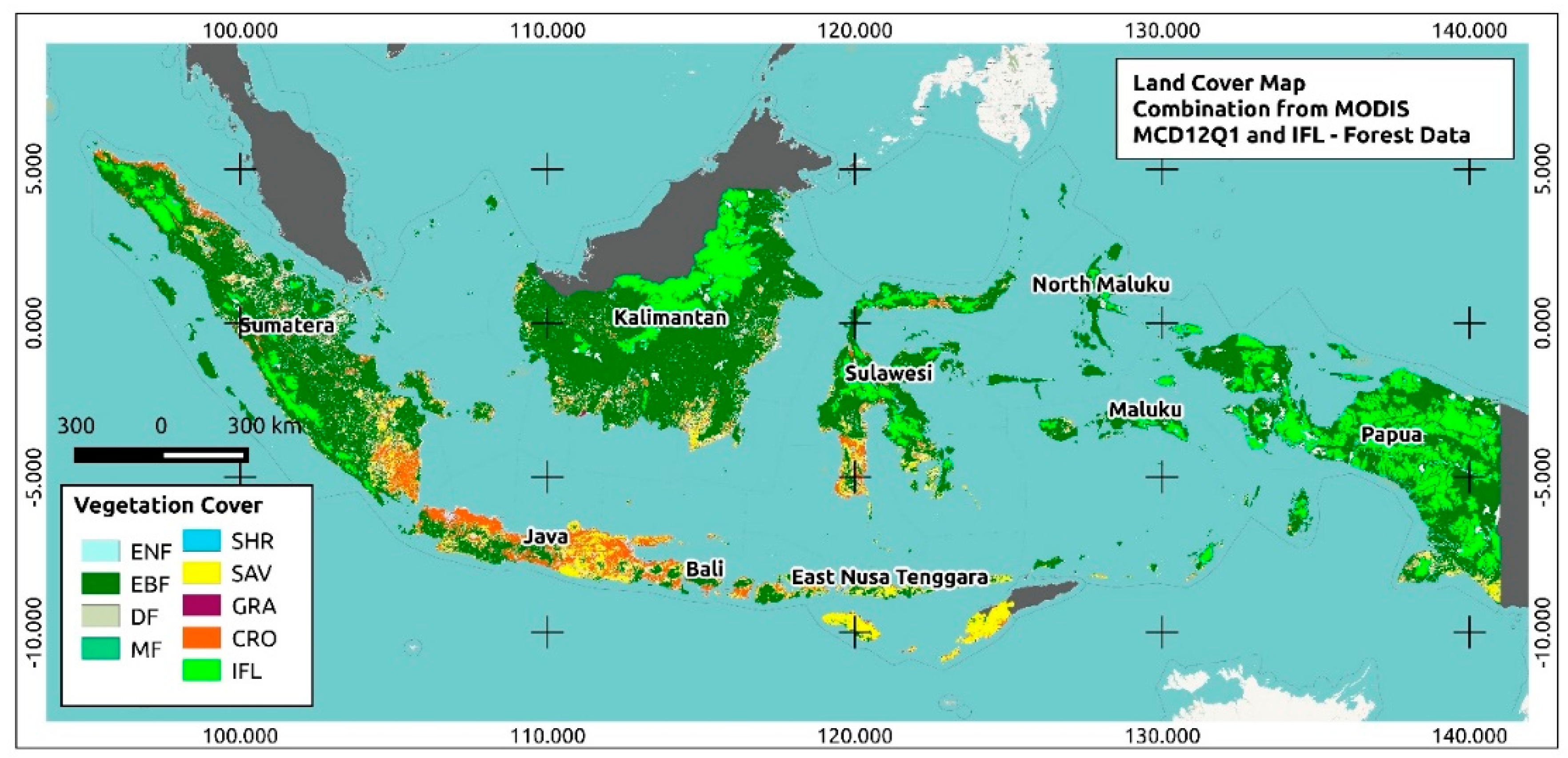
3.1.3. Vegetation Cover Types

The type 2 University of Maryland’s (UMD) vegetation cover scheme in MODIS MCD12Q1 [47] categories mainly divide the vegetation cover types into forestland, shrubland, savannas, and non-vegetated state. The forestland type was classified based on the combination between the leaf seasonality, i.e., evergreen and deciduous forest and leaf type, i.e., needle-leaf and broadleaf forest while mixed forest is a forest area with mixture of different type of forests while intact forest landscape (IFL) data [48] represents the intact and undisturbed forest areas. The combination of varying forest types made up of almost 88% of vegetation cover in Indonesia which 69.9% of them is the evergreen broadleaf forest (Table 1) with Dipterocarpaceae dominance. The remaining 12% of the vegetation covers were represented by the tree-less biomes and croplands. The treeless biomes were categorized based on their type of understory cover, such as shrublands, savannas, and grasslands, where half of the proportion of treeless biomes in Indonesia are occupied by savannas. The savanna lands in East Nusa Tenggara are usually covered by the patches of woody vegetation, herbs, and grass and used for agricultural and cattle purposes [49].
To obtain information on the corresponding vegetation cover types, we combined the MODIS MCD12Q1 [47] with 500-m spatial resolution in the year 2001 and 2013 with the 2013 remnant forest from IFL data. The type 2 UMD scheme includes 14 land cover classes, and the IFL data includes two classes of forested and deforestation. With the aim of simplifying land cover categories and extracting vegetation-related classes, the ‘water’, ‘urban and built up’, and ‘barren or sparsely vegetated’ classes in the MCD12Q1 Type 2 UMD scheme and the ‘deforestation’ classes were removed. Further class merging was conducted to simplify the LC classes and aggregate the similar LC; the lower level classes such as ‘deciduous broadleaved forest’ and ‘deciduous needleleaf forest’ were merged into ‘deciduous forest’. Another merging was also conducted of the ‘savanna’ and ‘woody savanna’ classes into the ‘savanna’ class, and the ‘closed shrublands’ and ‘open shrublands’ classes into the ‘shrublands’ class. In total, nine classes were retained for zonal statistics analysis (Table 1; Map in Figure 1).
Before combining the MCD12Q1 data with IFL data, we mapped non-changed land cover using the MCD12Q1 of years 2001 and 2013. This was performed to ensure the validity of statistical values, especially when performing zonal statistics.

3.2. Methods

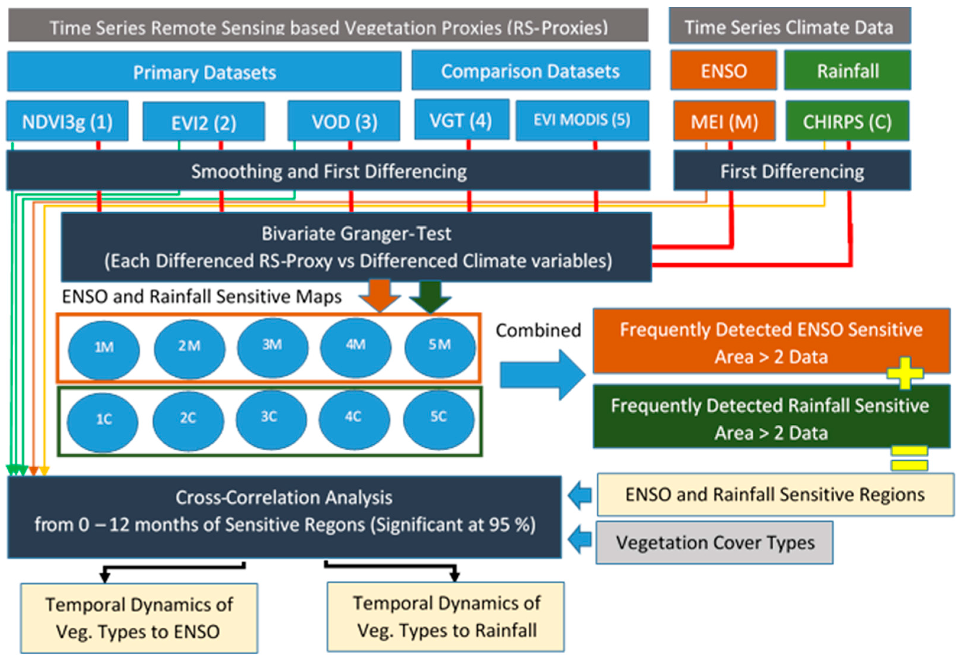
3.2.1. Bivariate Granger Causality

The regions that were identified as being sensitive in this study were defined as areas with dynamic time series values shown to be significantly influenced by climatic variables. The regions sensitive to ENSO and rainfall were identified using the Granger test compiled in the Lmtest R package [50], with the assumption that the fluctuation in the time series remote sensing values could be predicted by past time series values of ENSO indices and rainfall intensity with a certain lag. In this case, we used the MEI (ENSO) and CHIRPS (rainfall) as the representation of the dependent variables (x) while pixel values of RS proxies were considered as the independent variables (y). The Granger causality analysis was named after its inventor, Granger [51], and follows two assumptions: (1) the effect of the cause happens sometime later (indicated by time lag) and (2) the cause (X) contains information that can help predict the value of Y [52].
Based on previous assumptions, the implementation of Granger causality analysis in the Lmtest package was performed by comparing F-test results of two Wald tests from (1) an unrestricted model where the Y-variable was explained by including X-variables besides the values of Y alone at a certain lag, and (2) the restricted model where the Y-variable was explained using the previous value of Y itself. The sensitive area is indicated by a p-value below 0.05 (95% level of significance). This p-value indicates that there is less than a 5% probability of getting an opposite result when rejecting the null hypothesis that the x-variable does not contribute to the prediction of the y-variables. The lag order used in this analysis was selected from the lowest value of Akaike information criterion (AIC) from 0 to 12 months and conducted in the pixel-based analysis.
The main necessity for conducting Granger causality analysis is that the time series variables should be stationary. However, time series data from remote sensing observation are often depicted as non-stationary characteristics with the components of trend and seasonality [17]. Therefore, before initiating the Granger causality analysis, we transformed the original data into stationary ones by calculating the first difference in time series data.
The bivariate Granger test conducted between climate variables of the MEI (ENSO) and CHIRPS (rainfall) against five RS proxies generated a total of five ENSO sensitivity maps and five rainfall sensitivity maps with values ranging from 0 (not sensitive) to 1 (sensitive). From these sensitivity maps, the frequency maps of ENSO and rainfall were separately derived by combining the sensitivity maps through raster calculation, resulting in a frequency of 0 (not sensitive) to 5 (detected by all data). As the spatial resolutions of RS proxies are different, a down scaling process for MODIS and SPOT-VGT data from 1-km spatial resolution to 8-km spatial resolution was conducted by resampling with interpolation of the nearest neighbors and upscaling VOD data by disaggregating the pixel size from 25-km to 8-km spatial resolution. Lastly, we defined the ENSO- and rainfall-sensitive areas as the intersection of ENSO and rainfall frequency maps detected by at least two data types on each frequency map.

3.2.2. Cross-Correlation Function (CCF) from 0 to 12 Months

Cross-correlation function (CCF) analysis was performed by taking the average of significant correlation analysis (p-value < 0.05) with a lag of 0–12 months in the ENSO- and rainfall-sensitive areas. The CCF analysis aimed to assess the response of sensitive regions and to understand the process of MEI and rainfall in affecting the value of RS proxies over different vegetation cover types. The cross-correlation was executed in RStudio employing the base function for cross-correlation analysis. We used difference data because CCF also required the data to be in the stationary form.
The overall processing flow of this research is summarized in Figure 3.

4. Results

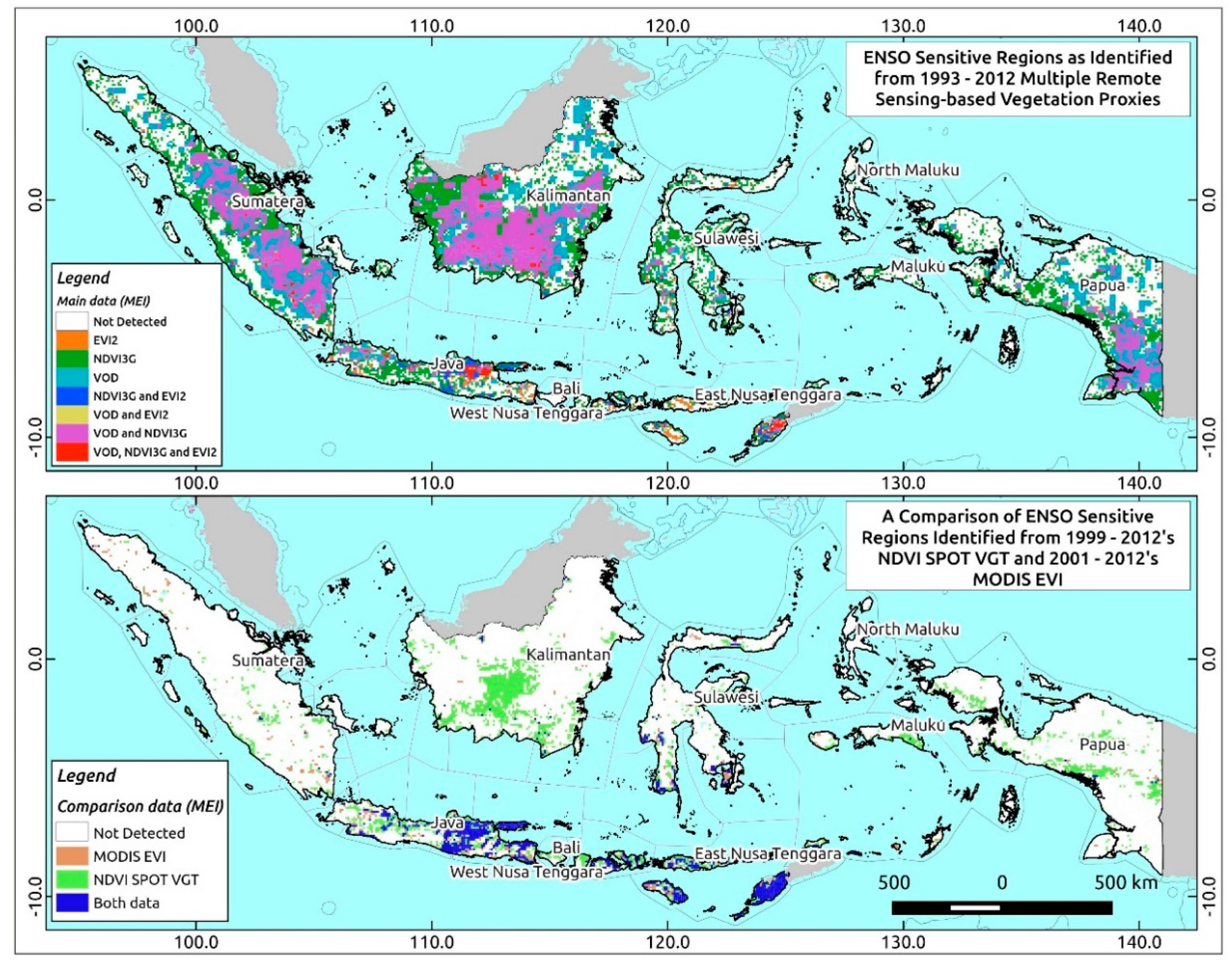
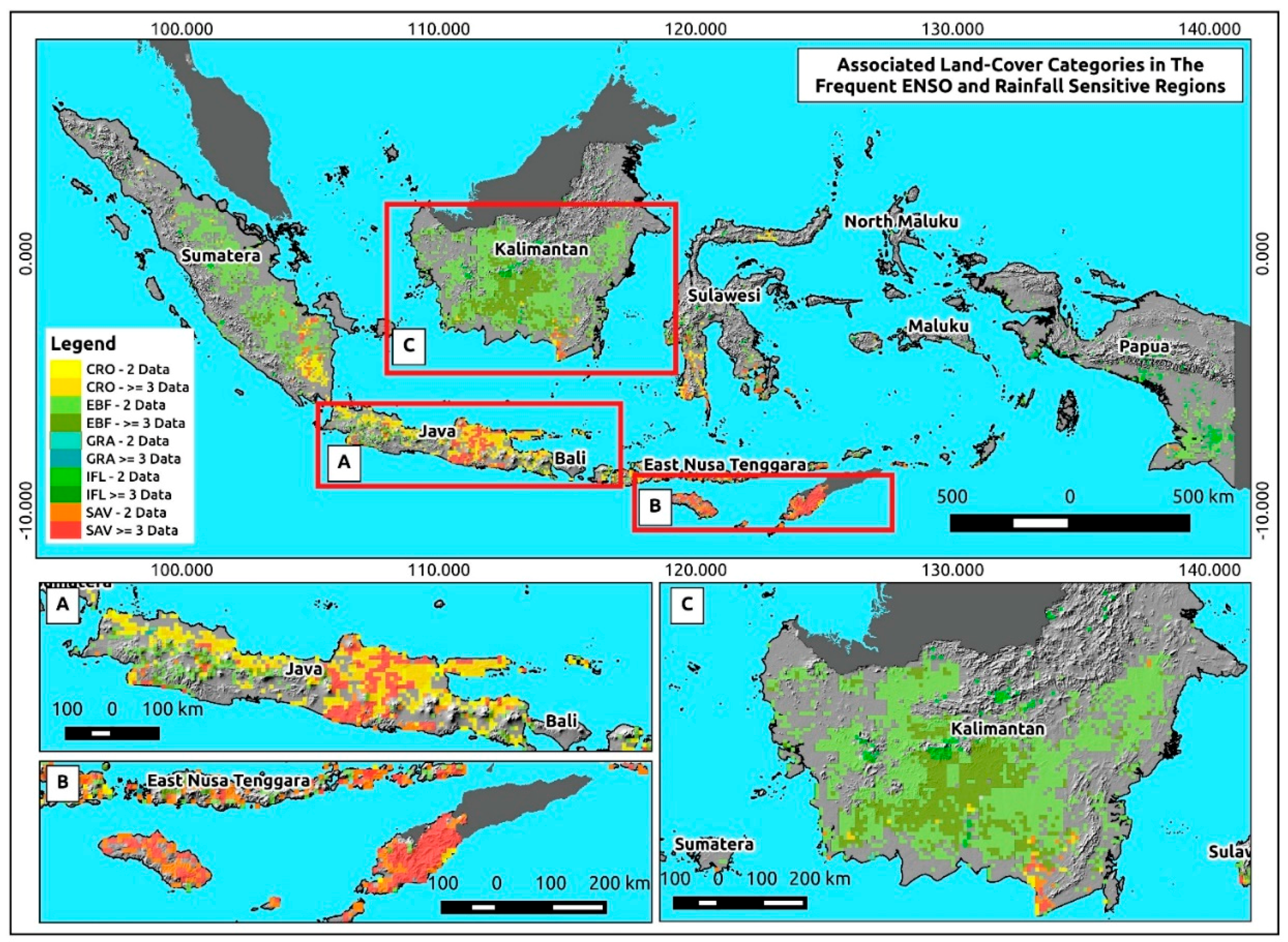
4.1. Identified ENSO- and Rainfall-Sensitive Regions in Indonesia

The Granger test analysis was performed between the vegetation proxies from remote sensing data (RS proxies) and climate variables of the MEI and CHIRPS (rainfall) data. Granger analysis for each data type was conducted separately, and the results were plotted on maps intersected at 8-km spatial resolution for the 1992–2012 EVI2 VIP, NDVI3g, and VOD, while ENSO-Granger analysis for SPOT VGT and MODIS EVI were used as ancillary data. The ENSO-Granger causality analysis performed on NDVI3g, VOD, and EVI2 from 1993 to 2012 yielded different spatial patterns for each dataset. NDVI3g and VOD data detected 44–47% of the total study area as being sensitive to ENSO, while EVI2 identified only 9.3% of the entire study area as being sensitive to ENSO, which is markedly less. However, the EVI2 result is comparable to the 2001–2012 MODIS EVI analysis that yielded a similar percentage (8.1%) and similar spatial pattern. Another analysis using 1999–2012 VGT NDVI data also detected less area (18.9% of the total area) and its spatial distribution was almost identical to the EVI observation. Agreement in the spatial pattern of ENSO-sensitivity based on NDVI3g and VOD data appeared in Sumatera, the southern part of Borneo, Java, West and Nusa Tenggara and the southern part of Papua, while SPOT VGT, VIP EVI2, and MODIS EVI shared similar spatial distributions in the East Java and Nusa Tenggara islands (Figure 4). On the final map, a combination of those three primary datasets and the ancillary datasets revealed that the areas detected by all datasets were located in the eastern part of Java and East Nusa Tenggara.
The CHIRPS (rainfall)-Granger causality analysis applied to the remote sensing datasets detected more prominent areas corresponding to rainfall intensity compared to for ENSO (Figure 5). Approximately 60–60.4% of the total study area was identified as being rainfall-sensitive using 1993–2012 VOD and NDVI3g as the primary datasets, while analysis with the 1999–2012 VGT and 2001–2012 MODIS EVI identified fewer regions with 45.6–60.2% of the total area being sensitive to CHIRPS (rainfall) intensity. However, VIP EVI2 showed quite distinct sensitive area percentage than the rest of the RS proxies with only 25.6%. Similar portions of rainfall-sensitive areas were identified in the datasets, especially in VOD, NDVI3g, MODIS EVI, and SPOT VGT, which shared identical spatial distributions of rainfall-sensitive areas in Java, Sumatera, Southern Borneo, the southwestern part of Sulawesi, and the southern part of Papua. Further comparison with VIP EVI2 showed that the spatial distribution of the sensitive areas agreed on Java and the small islands across West Nusa Tenggara and East Timor. This distribution of sensitive regions from EVI2 is almost identical to the distribution of the ENSO-sensitive region of EVI2 in the previous analysis.
The results of multiple analyses of areas sensitive to ENSO and rainfall allowed us to map the areas that were commonly/frequently identified as climate-sensitive in multiple datasets. Combining the maps of sensitive areas from primary and ancillary datasets produced the frequent sensitivity maps with values from 0 (non-sensitive) to 5 (detected in all datasets) for the ENSO and rainfall maps (Figure 6). By linking vegetation type to frequencies on both sensitivity maps, a further association of the highly-sensitive vegetation region could be determined. It was found that savanna (SAV) had the highest agreement among different datasets with 41.27% and 51.93% being identified as MEI (ENSO)- and CHIRPS (rainfall)-sensitive areas, respectively, by more than three datasets (Table 2). Cropland was identified as having the second highest agreement with 17.34% and 42.64% being in spatial agreement for MEI (ENSO) and CHIRPS (rainfall). Overall, compared to the frequency analysis conducted side-by-side, spatial agreement between the various remote sensing sensors was higher for the rainfall sensitivity map than for the ENSO sensitivity map, indicating a higher percentage of areas with overlapping sensitivity indicated by at least three datasets.
The MEI (ENSO) and CHIRPS (rainfall) sensitivity maps from various sensors showed that several areas had frequencies corresponding to both ENSO and changing rainfall. The sensitive areas detected by more than two datasets in MEI (ENSO) and CHIRPS (rainfall)-Granger analysis were located in East Java, the lowlands of Sumatera, southern Kalimantan, Southwestern Sulawesi, and Southern Papua (Figure 7). The intersection between land cover data and the frequently identified sensitive areas revealed that several land cover classes corresponded strongly to both ENSO and rainfall (Table 3). The findings also showed that savanna (SAV) vegetation class type was highly affected by ENSO and rainfall. Interestingly, more than two RS proxies mapped a total of 53% of savanna cover as being sensitive. Further, cropland (CRO) and grassland (GRA) showed correspondence of 36.7% and 26.4% of total areas to ENSO and rainfall, respectively.

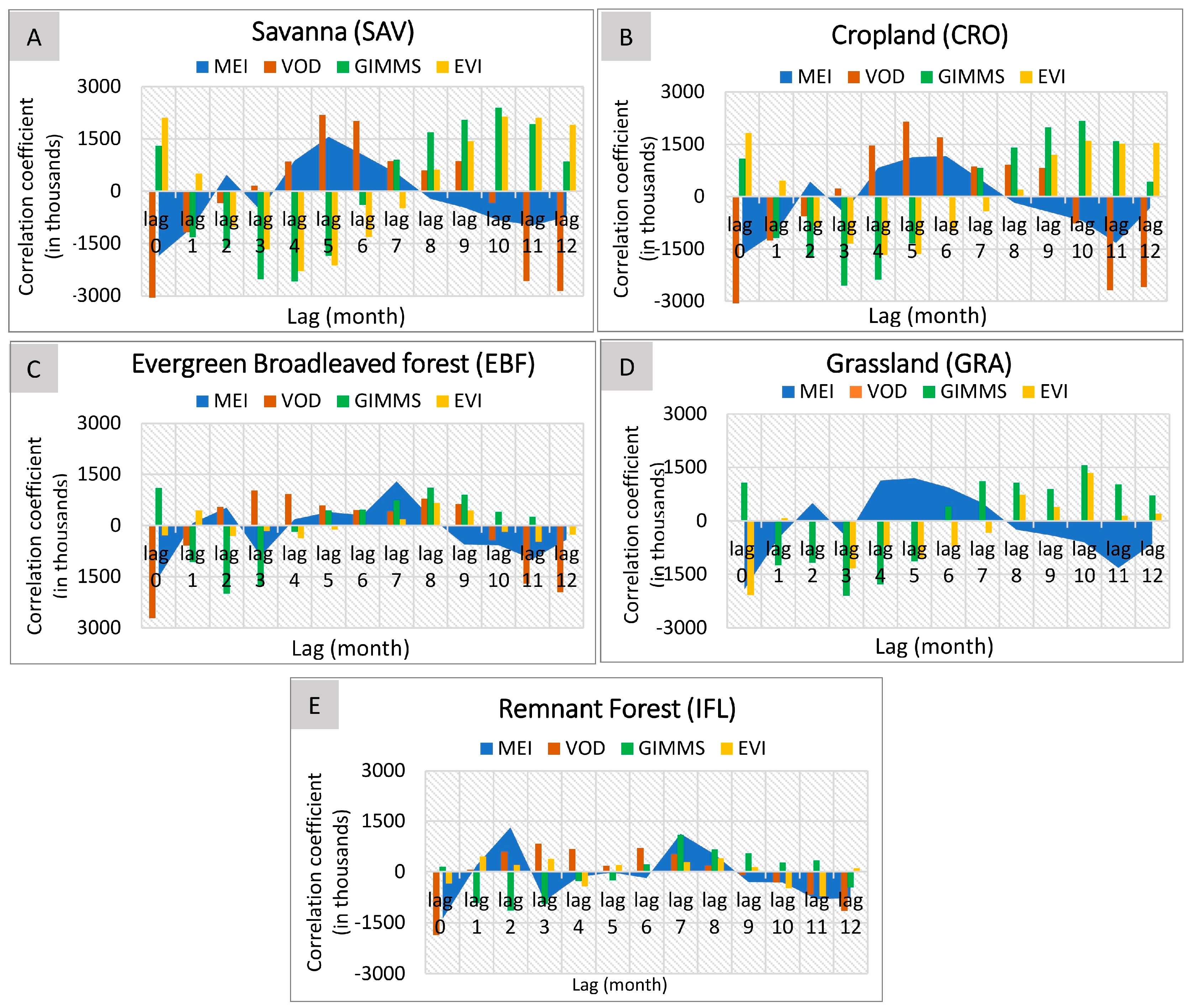
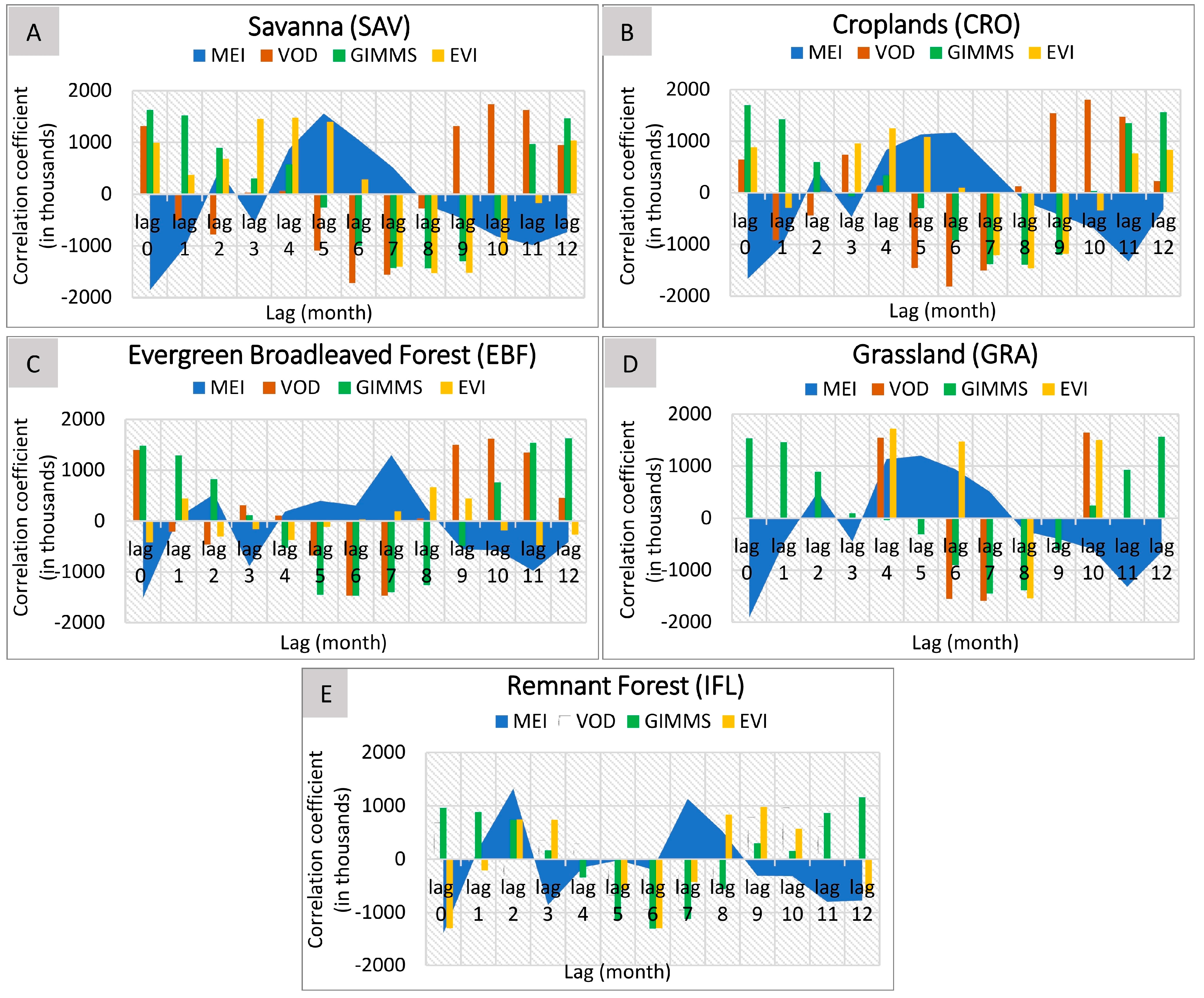
4.2. Response of ENSO-Rainfall Sensitive Regions in Indonesia

Overall, the average CCF coefficients between the MEI (ENSO) against RS proxies and RS proxies against CHIRPS (rainfall) for 0–12 months at different land cover types yielded low correlation coefficients. The correlation coefficients ranged from −0.19 to 0.18 for RS proxies versus ENSO and −0.3–0.2 for RS proxies versus rainfall. Even though the CCF coefficients were low, tracking the progression of the CCF coefficient values between RS proxies versus CHIRPS-rainfall and RS proxies versus the MEI (ENSO) compared with the CCF coefficients between the MEI (ENSO) and CHIRPS (rainfall) for different land cover types allowed us to depict temporal characteristics of how ENSO affected rainfall and sequentially controlled variation in NDVI values throughout the years.
A similar pattern of ENSO-rainfall CCF coefficients for different land cover types (plotted as a blue area in Figure 8 and Figure 9), excluding the IFL type, were presented in CCF results. Significantly highly negative correlations (p-value < 0.05) occurred with a lag of 0–2 months. This suggests that as the ENSO magnitude grew larger, rainfall intensity grew smaller over the same period. Further, CCF patterns in most of land cover classes showed a strong positive correlation starting from +3 months and peaking at +5 to +6 months, although a weaker negative relationship was shown at a lag of 11 months. However, remnant forest (IFL) did not share a similar temporal pattern with other classes. The CCF coefficients of ENSO-rainfall in IFL remained low to showing no correlation after displaying identical negative relationships from the first months to a time lag of +6 months, where they started exhibiting a positive correlation.
CCF analysis between CHIRPS (rainfall) and RS proxies displayed a relatively distinct temporal pattern in VOD compared to EVI2 and NDVI3g. Generally, the CCF graphs of VOD against rainfall showed a similar pattern of the MEI to rainfall where it showed negative correlations during the first two months and positive correlation started and then sometimes peaked between +3 and +5 months (Figure 8). In contrast to VOD, NDVI3g and EVI showed positive correlations with rainfall during the first months of ENSO with the highest negative correlations at lag +3 to +5 months. This may suggest that (1) rainfall change did not simultaneously affect vegetation water content; or (2) when ENSO negatively affected rainfall at lag of 0–1 months, most vegetation types, such as savanna, cropland, and forest (aboveground and remnant forest), were still able to maintain water in their biomass that was indicated by negative correlations between rainfall and VOD data during lag of 0–1 months.
There are few differences worth emphasizing from the CCF graphs among different types of vegetation cover. Among the CCF values of vegetation cover types, the average CCF coefficients between rainfall and RS proxies in the remnant forest were the smallest among other vegetation types. This may indicate that the effects of rainfall are insignificant to the greenness level of the remnant forest. Another difference is that there is an incomplete observation in the CCF-rainfall versus VOD due to its coarse spatial resolution where, in the area of grasslands, only a few coefficient lags appear in the graphs due to its small coverage area. Therefore, the incomplete CCF coefficient problem also appeared in the CCF-MEI ENSO vs. VOD for grassland types due to the same spatial resolution mismatching problem.
Different responses in the CCF graphs between the MEI-ENSO and RS proxies were observed (Figure 9). Significant positive correlations were observed in the first months, and the highest positive correlation appeared around the latter months (+6–12 months). Different from the ENSO-rainfall CCF graph, which showed the first negative correlations at lag 0–2 months, ENSO lagged RS proxy values negatively in different vegetation cover types at +6–11 months. This indicates that there was different time lag when ENSO started affecting rainfall and was further reflected in the photosynthetic activities of vegetation or greenness level. The CCF graphs also show initial negative correlations in VOD at lag +1 month and a peak at lag 6 or 7 months. The first negative correlations in VOD suggest that most of the changes in vegetation water content came first and then were followed by a decline in photosynthetic activity or greenness level later.

5. Discussion

The spatial distribution of sensitive areas obtained from multi-sensor remote sensing approaches showed the southern part of Indonesia, including some parts of Sumatera, Java Island, the southern part of Kalimantan Island, the islands in Nusa Tenggara, and the southern Part of Papua to be ENSO- and rainfall-sensitive areas. This finding corroborates those of previous studies showing these regions to be the two climate regions sensitive to rainfall with seasonality heavily influenced by ENSO, which affects the area until the latter months of the year [53,54]. The union of ENSO-sensitive areas from multi-sensor remote sensing data also corresponds with the same analysis in Erasmi et al. [15], although the intersection of sensitive regions yielded different spatial patterns for ENSO- and rainfall-sensitive vegetation cover types. Eastern part of Java is one of the hotspot areas where most of the data agreed by more than three RS data which identified this region as the ENSO and rainfall sensitive region. The identification of East Java as an identified region is in line with a specific local study that identified this area for being massively affected by climate extremes and having experienced decreases in rainfall and prolonged droughts during ENSO [55].
Identification of sensitive regions by combining multiple remote sensing datasets revealed a high similarity between NDVI3g and VOD measurements, while EVI detected fewer areas compared with previous datasets. The high agreement between NDVI3g and VOD is supported by a study showing that NDVI represents the vegetation and moisture condition [56] which is similar to the findings presented in VOD. On the other hand, according to Pettorelli et al. [25], EVI is more sensitive to structural change in vegetation canopy due to its wider dynamic range over NDVI-saturated areas. The combination of VOD, NDVI, and EVI led to identification of savanna as the vegetation type most influenced by ENSO and rainfall in Indonesia because drastic structural changes are observed in response to different climate conditions.
Savanna in Indonesia is a treeless biome in arid climate and covered with grass (Figure 10). The stability of this biome depends on rainfall and fire cycles [57,58,59,60]. The ENSO warm and cold phases offer a cycle of drought and intensified rainfall that controls the savanna dynamics, making this biome the most appropriate ecosystem to examine for a response to the ENSO effect. The intensified warm ENSOs with prolonged drought and increased temperature can triggered more frequent fire thus further reducing the tree density in savanna and impacting the ecosystem services and the biodiversity. In addition, similar reductions of tree density due to drought and fire can be expected from the shifting of tropical forest into savanna-like ecosystems where it may difficult to restore. The fact that some evergreen broadleaf forests in Sumatera were identified as an ecosystem that is sensitive to ENSO can also be attributed to the possible historical ENSO-related forest fires that are widely suspected to enhance the temporal shift of forest characteristics into a savanna-like environment [61]. The ENSO- and rainfall-sensitivity in this study can be used to identify areas that require proper mitigation and for anticipating and possibly avoiding unrecoverable transformation of ecosystems.
The temporal graphics of CCF among the different vegetation cover types exposed the progress of how MEI-ENSO affects vegetation, especially in the ENSO- and rainfall-sensitive areas. MEI (ENSO) first affected rainfall at lag 0 months, as indicated with strong negative correlation and that ENSO-induced changes in rainfall affected vegetation (indicated by positive correlation) at around 5–6 months later in the graphs. The persistent effect up to four months after MEI to rainfall in the CCF results is similar to that in Hendon [62]. It was also shown that stronger correlations were found in CCF between rainfall and RS proxies compared to CCF between MEI and RS proxies.
An in-depth look at the time lag spatial distribution of significant correlations revealed the influence of land cover and terrain characteristics. Figure 11 showed the lag distribution of negative correlations between rainfall to RS proxies and MEI ENSO to RS proxies with shaded relief by SRTM data in the background. The control of terrain configurations can be seen especially at the time lag between NDVI3g to rainfall. Topography differences controlled the distribution of the timing of lags and created a distinct spatial pattern of the lag time when strong negative correlation occurred. In NDVI3g lag to rainfall (Figure 11), an area at high elevation experienced an earlier strong, negative correlation compared to a lowland area. The relationship between terrain characteristics and rainfall intensities during the ENSO period in Java Island have been discussed previously [63]. Therefore, further studies of the effects of topography are needed to fully understand the vegetation and terrain relationships that control the impact of ENSO.

6. Conclusions

The combination of analysis from multiple remote sensing proxies such as NDVI3g, EVI2, and VOD datasets (RS Proxies) in 1993–2012, complemented by SPOT VGT in 1999–2012 and MODIS EVI in 2001–2012 yielded the spatial patterns of ENSO- and rainfall-sensitive regions. There are several key points that can be drawn from the results, as follows:
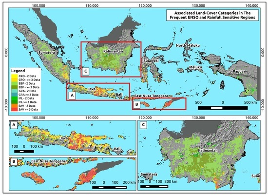
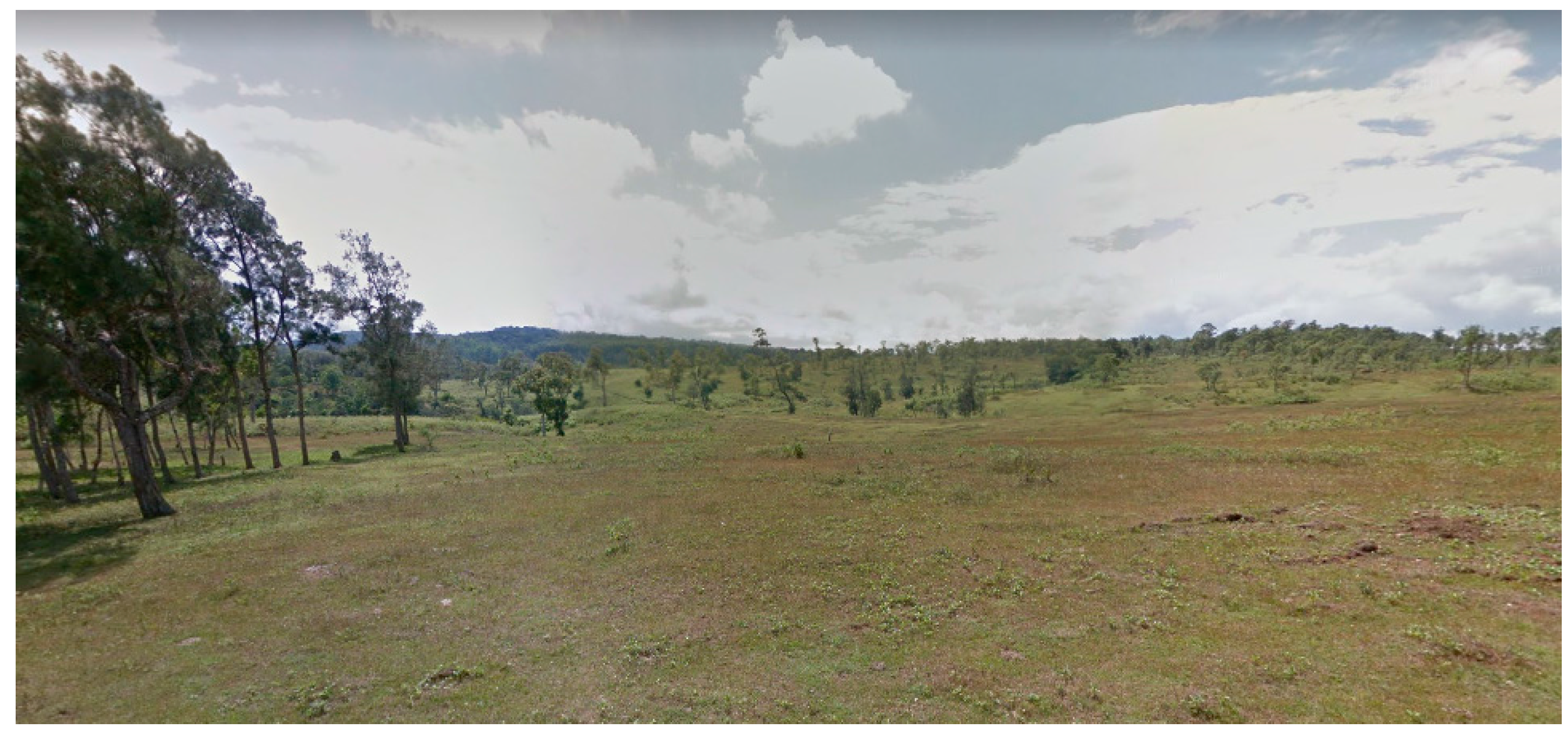
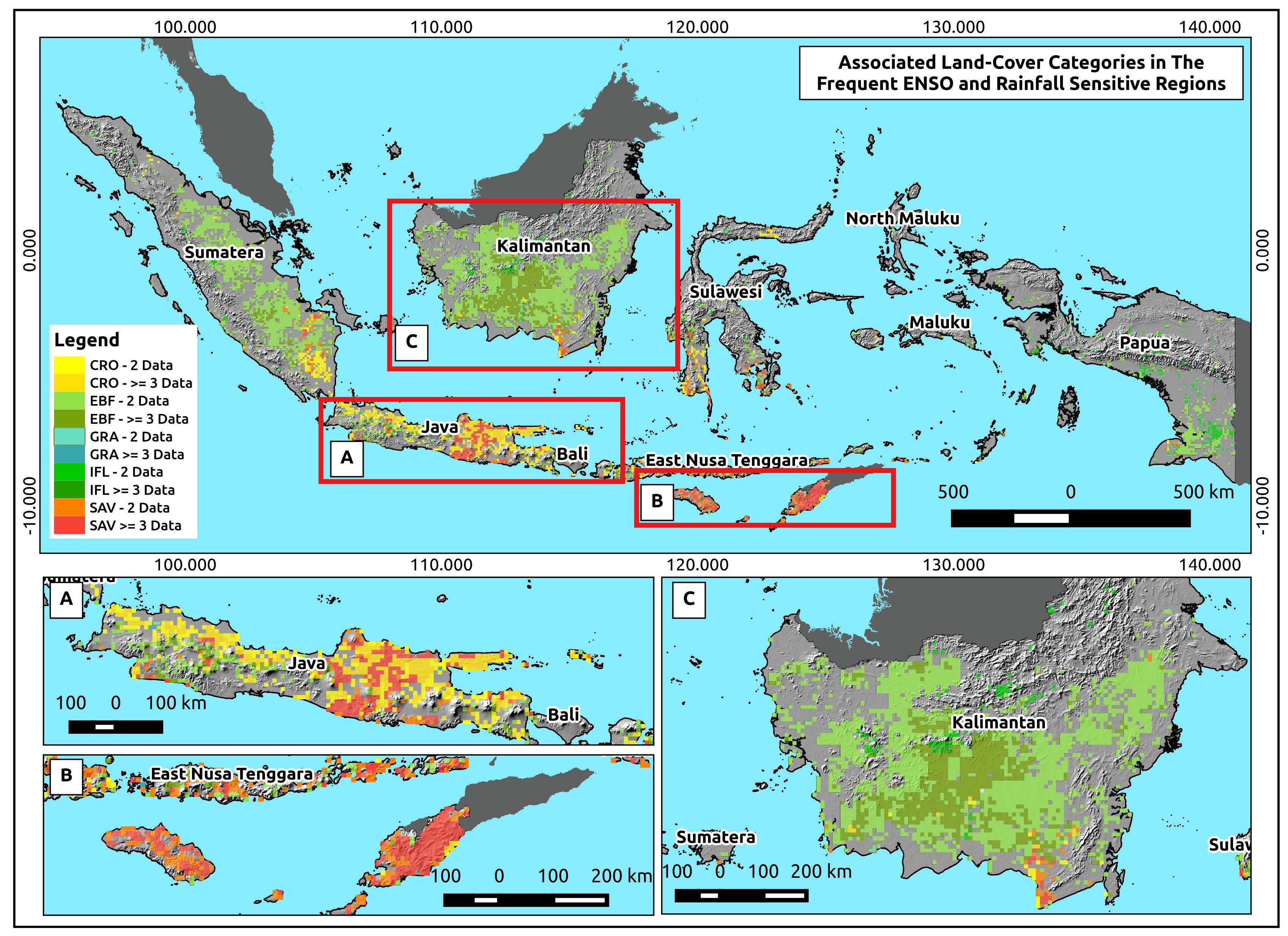
  • Combinations of MEI (ENSO) and CHIRP-rainfall sensitive areas detected from Granger causality analysis frequently identified savanna, cropland, evergreen broadleaved forest, grassland, and remnant forest (IFL) as sensitive regions. The drastic phenology change of savanna, especially during drought and wet phases, created the strong relationship between ENSO and savanna environments, which was captured by various remote sensing-based vegetation proxies.
  • The temporal graphs from the CCF analysis revealed that MEI (ENSO) affected the CHIRPS-rainfall values in the first months for which its variation further affected the values of RS proxies.
  • The spatial distribution of time lag coefficients from CCF suggested that not only land cover types, but also topography, played an essential role in generating the spatial patterns.
The results drives the need for further studies on other confounding variables that might affect the relationships between MEI and RS proxies. In addition, under the intensified ENSO due to the influence of global warming, these sensitive regions are becoming more susceptible to vegetation cover changes and, thus, endangering species biodiversity and ecosystem services and need to be properly mitigated.

Acknowledgments

The authors would like to thank all who freely provided data through their repositories, Robert Parinussa, and Yi Y. Liu who provided access to the VOD data for Indonesia. We thank Karlina Indraswari for kind suggestions on the manuscript, and lastly, we thank MEXT-Monbukagakusho for providing the scholarships to the first author in order to conduct this research.

Author Contributions

S.A. designed the research, performed the analysis and drafted the manuscript. Y.Y. and Y.H. made comments and checked the manuscript. X.Z. was involved in generating ideas and data sharing.

Conflicts of Interest

The authors declare no conflicts of interest and the founding sponsors had no role in the design of the study; in the collection, analyses, or interpretation of data; in the writing of the manuscript; or in the decision to publish the results.

References

  1. Intergovernmental Panel on Climate Change (IPCC). Climate Change 2014–Impacts, Adaptation and Vulnerability: Regional Aspects; Cambridge University Press: Cambridge, UK, 2014. [Google Scholar]
  2. Sheffield, J.; Wood, E.F. Projected changes in drought occurrence under future global warming from multi-model, multi-scenario, IPCC ar4 simulations. Clim. Dyn. 2008, 31, 79–105. [Google Scholar] [CrossRef]
  3. Collins, M.; An, S.-I.; Cai, W.; Ganachaud, A.; Guilyardi, E.; Jin, F.-F.; Jochum, M.; Lengaigne, M.; Power, S.; Timmermann, A. The impact of global warming on the tropical Pacific Ocean and El niño. Nat. Geosci. 2010, 3, 391–397. [Google Scholar] [CrossRef]
  4. Cai, W.; Santoso, A.; Wang, G.; Yeh, S.-W.; An, S.-I.; Cobb, K.M.; Collins, M.; Guilyardi, E.; Jin, F.-F.; Kug, J.-S. Enso and greenhouse warming. Nat. Clim. Chang. 2015, 5, 849–859. [Google Scholar] [CrossRef] [Green Version]
  5. Kirono, D.G.; Tapper, N.J.; McBride, J.L. Documenting indonesian rainfall in the 1997/1998 El nino event. Phys. Geogr. 1999, 20, 422–435. [Google Scholar]
  6. Arcari, P.; Tapper, N.; Pfueller, S. Regional variability in relationships between climate and dengue/DHF in indonesia. Singap. J. Trop. Geogr. 2007, 28, 251–272. [Google Scholar] [CrossRef]
  7. Murdiyarso, D.; Adiningsih, E.S. Climate anomalies, indonesian vegetation fires and terrestrial carbon emissions. Mitig. Adapt. Strateg. Glob. Chang. 2007, 12, 101–112. [Google Scholar] [CrossRef]
  8. Boisvenue, C.; Running, S.W. Impacts of climate change on natural forest productivity–evidence since the middle of the 20th century. Glob. Chang. Biol. 2006, 12, 862–882. [Google Scholar] [CrossRef]
  9. Allen, C.D.; Macalady, A.K.; Chenchouni, H.; Bachelet, D.; McDowell, N.; Vennetier, M.; Kitzberger, T.; Rigling, A.; Breshears, D.D.; Hogg, E.T. A global overview of drought and heat-induced tree mortality reveals emerging climate change risks for forests. For. Ecol. Manag. 2010, 259, 660–684. [Google Scholar] [CrossRef]
  10. Holmgren, M.; Scheffer, M.; Ezcurra, E.; Gutiérrez, J.R.; Mohren, G.M. El niño effects on the dynamics of terrestrial ecosystems. Trends Ecol. Evol. 2001, 16, 89–94. [Google Scholar] [CrossRef]
  11. Kirono, D.G.; Tapper, N.J. Enso rainfall variability and impacts on crop production in indonesia. Phys. Geogr. 1999, 20, 508–519. [Google Scholar]
  12. Naylor, R.L.; Falcon, W.P.; Rochberg, D.; Wada, N. Using El Nino/Southern Oscillation climate data to predict rice production in indonesia. Clim. Chang. 2001, 50, 255–265. [Google Scholar] [CrossRef]
  13. Naylor, R.L.; Battisti, D.S.; Vimont, D.J.; Falcon, W.P.; Burke, M.B. Assessing risks of climate variability and climate change for indonesian rice agriculture. Proc. Natl. Acad. Sci. USA 2007, 104, 7752–7757. [Google Scholar] [CrossRef] [PubMed]
  14. Gutman, G.; Csiszar, I.; Romanov, P. Using NOAA/AVHRR products to monitor El Nino impacts: Focus on Indonesia in 1997–1998. Bull. Am. Meteorol. Soc. 2000, 81, 1189–1205. [Google Scholar] [CrossRef]
  15. Erasmi, S.; Propastin, P.; Kappas, M.; Panferov, O. Spatial patterns of NDVI variation over Indonesia and their relationship to ENSO warm events during the period 1982–2006. J. Clim. 2009, 22, 6612–6623. [Google Scholar] [CrossRef]
  16. Tucker, C.; Sellers, P. Satellite remote sensing of primary production. Int. J. Remote Sens. 1986, 7, 1395–1416. [Google Scholar] [CrossRef]
  17. Pinzon, J.E.; Tucker, C.J. A non-stationary 1981–2012 AVHRR NDVI3g time series. Remote Sens. 2014, 6, 6929–6960. [Google Scholar] [CrossRef]
  18. Hawinkel, P.; Thiery, W.; Lhermitte, S.; Swinnen, E.; Verbist, B.; Van Orshoven, J.; Muys, B. Vegetation response to precipitation variability in East Africa controlled by biogeographical factors. J. Geophys. Res. Biogeosci. 2016, 121, 2422–2444. [Google Scholar] [CrossRef]
  19. Piao, S.; Fang, J.; Zhou, L.; Ciais, P.; Zhu, B. Variations in satellite-derived phenology in china’s temperate vegetation. Glob. Chang. Biol. 2006, 12, 672–685. [Google Scholar] [CrossRef]
  20. Revadekar, J.; Tiwari, Y.K.; Kumar, K.R. Impact of climate variability on NDVI over the Indian region during 1981–2010. Int. J. Remote Sens. 2012, 33, 7132–7150. [Google Scholar] [CrossRef]
  21. Epiphanio, J.N.; Huete, A.R. Dependence of NDVI and SAVI on sun/sensor geometry and its effect on fAPAR relationships in Alfalfa. Remote Sens. Environ. 1995, 51, 351–360. [Google Scholar] [CrossRef]
  22. Huete, A.; Didan, K.; Miura, T.; Rodriguez, E.P.; Gao, X.; Ferreira, L.G. Overview of the radiometric and biophysical performance of the modis vegetation indices. Remote Sens. Environ. 2002, 83, 195–213. [Google Scholar] [CrossRef]
  23. Rocha, A.V.; Shaver, G.R. Advantages of a two band EVI calculated from solar and photosynthetically active radiation fluxes. Agric. For. Meteorol. 2009, 149, 1560–1563. [Google Scholar] [CrossRef]
  24. Jiang, Z.; Huete, A.R.; Didan, K.; Miura, T. Development of a two-band enhanced vegetation index without a blue band. Remote Sens. Environ. 2008, 112, 3833–3845. [Google Scholar] [CrossRef]
  25. Pettorelli, N.; Vik, J.O.; Mysterud, A.; Gaillard, J.-M.; Tucker, C.J.; Stenseth, N.C. Using the satellite-derived NDVI to assess ecological responses to environmental change. Trends Ecol. Evol. 2005, 20, 503–510. [Google Scholar] [CrossRef] [PubMed]
  26. Owe, M.; de Jeu, R.; Walker, J. A methodology for surface soil moisture and vegetation optical depth retrieval using the microwave polarization difference index. IEEE Trans. Geosci. Remote Sens. 2001, 39, 1643–1654. [Google Scholar] [CrossRef]
  27. Liu, Y.Y.; Dijk, A.I.; McCabe, M.F.; Evans, J.P.; Jeu, R.A. Global vegetation biomass change (1988–2008) and attribution to environmental and human drivers. Glob. Ecol. Biogeogr. 2013, 22, 692–705. [Google Scholar] [CrossRef]
  28. Liu, Y.Y.; de Jeu, R.A.; McCabe, M.F.; Evans, J.P.; van Dijk, A.I. Global long-term passive microwave satellite-based retrievals of vegetation optical depth. Geophys. Res. Lett. 2011, 38. [Google Scholar] [CrossRef]
  29. Amien, I.; Rejekiningrum, P.; Pramudia, A.; Susanti, E. Effects of Interannual climate variability and climate change on rice yield in Java, Indonesia. In Climate Change Vulnerability and Adaptation in Asia and the Pacific; Springer: Beilin, Germany, 1996; pp. 29–39. [Google Scholar]
  30. MacDicken, K.; Jonsson, Ö.; Piña, L.; Maulo, S.; Contessa, V.; Adikari, Y.; Garzuglia, M.; Lindquist, E.; Reams, G.; D’Annunzio, R. Global Forest Resources Assessment 2015: How Are the World’s Forests Changing? Food and Agriculture Organization: Rome, Italy, 2016. [Google Scholar]
  31. EcoCast. Available online: https://ecocast.arc.nasa.gov/data/pub/gimms/ (accessed on 13 January 2017).
  32. Jönsson, P.; Eklundh, L. Timesat—A program for analyzing time-series of satellite sensor data. Comput. Geosci. 2004, 30, 833–845. [Google Scholar] [CrossRef]
  33. Didan, K.; Munoz, A.B.; Solano, R.; Huete, A. MODIS vegetation index user’s guide (MOD13 series). Available online: https://icdc.cen.uni-hamburg.de/fileadmin/user_upload/icdc_Dokumente/MODIS/MODIS_Collection6_VegetationIndex_UsersGuide_MOD13_V03_June2015.pdf (accessed on 14 March 2018).
  34. Jiang, Z.; Huete, A.R.; Kim, Y.; Didan, K. 2-band enhanced vegetation index without a blue band and its application to AVHRR data. Proc. SPIE 2007, 6679, 667905. [Google Scholar] [CrossRef]
  35. Meesters, A.G.; De Jeu, R.A.; Owe, M. Analytical derivation of the vegetation optical depth from the microwave polarization difference index. IEEE Geosci. Remote Sens. Lett. 2005, 2, 121–123. [Google Scholar] [CrossRef]
  36. Owe, M.; de Jeu, R.; Holmes, T. Multisensor historical climatology of satellite-derived global land surface moisture. J. Geophys. Res. Earth Surf. 2008, 113. [Google Scholar] [CrossRef] [Green Version]
  37. Liu, Y.Y.; Van Dijk, A.I.; De Jeu, R.A.; Canadell, J.G.; McCabe, M.F.; Evans, J.P.; Wang, G. Recent reversal in loss of global terrestrial biomass. Nat. Clim. Chang. 2015, 5, 470–474. [Google Scholar] [CrossRef]
  38. Flemish Institute for Technological Research (VITO). Available online: http://www.vito-eodata.be (accessed on 4 April 2017).
  39. Wolters, E.; Swinnen, E.; Toté, C.; Sterckx, S. Spot-VGT Collection 3 Products User Manual; Flemish Institute for Technological Research (VITO): Antwerp, Belgium, 2016. [Google Scholar]
  40. Huete, A.; Justice, C.; Van Leeuwen, W. MODIS vegetation index (MOD13). Algorithm Theor. Basis Doc. 1999, 3, 213. [Google Scholar]
  41. Stenseth, N.C.; Ottersen, G.; Hurrell, J.W.; Mysterud, A.; Lima, M.; Chan, K.S.; Yoccoz, N.G.; Ådlandsvik, B. Studying climate effects on ecology through the use of climate indices: The North Atlantic Oscillation, El Nino Southern Oscillation and beyond. Proc. R. Soc. Lond. B Biol. Sci. 2003, 270, 2087–2096. [Google Scholar] [CrossRef] [PubMed]
  42. Wolter, K. Mei Index (Current Update: 9 November 2017). Available online: https://www.esrl.noaa.gov/psd/enso/mei/table.html (accessed on 20 November 2017).
  43. Chirps. Available online: http://chg.geog.ucsb.edu/data/chirps/ (accessed on 4 January 2017).
  44. Funk, C.; Peterson, P.; Landsfeld, M.; Pedreros, D.; Verdin, J.; Shukla, S.; Husak, G.; Rowland, J.; Harrison, L.; Hoell, A. The climate hazards infrared precipitation with stations—A new environmental record for monitoring extremes. Sci. Data 2015, 2, 150066. [Google Scholar] [CrossRef] [PubMed]
  45. Katsanos, D.; Retalis, A.; Michaelides, S. Validation of a high-resolution precipitation database (CHIRPS) over Cyprus for a 30-year period. Atmos. Res. 2016, 169, 459–464. [Google Scholar] [CrossRef]
  46. Trejo, F.J.P.; Barbosa, H.A.; Peñaloza-Murillo, M.A.; Moreno, M.A.; Farías, A. Intercomparison of improved satellite rainfall estimation with chirps gridded product and rain gauge data over venezuela. Atmósfera 2016, 29, 323–342. [Google Scholar] [CrossRef]
  47. Friedl, M.A.; Sulla-Menashe, D.; Tan, B.; Schneider, A.; Ramankutty, N.; Sibley, A.; Huang, X. Modis collection 5 global land cover: Algorithm refinements and characterization of new datasets. Remote Sens. Environ. 2010, 114, 168–182. [Google Scholar] [CrossRef]
  48. Potapov, P.; Yaroshenko, A.; Turubanova, S.; Dubinin, M.; Laestadius, L.; Thies, C.; Aksenov, D.; Egorov, A.; Yesipova, Y.; Glushkov, I. Mapping the world’s intact forest landscapes by remote sensing. Ecol. Soc. 2008, 13, 51. [Google Scholar] [CrossRef]
  49. Russell-Smith, J.; Djoeroemana, S.; Maan, J.; Pandanga, P. Rural livelihoods and burning practices in savanna landscapes of nusa tenggara timur, eastern indonesia. Hum. Ecol. 2007, 35, 345–359. [Google Scholar] [CrossRef]
  50. Hothorn, T.; Zeileis, A.; Farebrother, R.W.; Cummins, C.; Millo, G.; Mitchell, D. Lmtest: Testing Linear Regression Models. R Package Version 0.9-34. Available online: https://cran.r-project.org/package=lmtest (accessed on 6 May 2017).
  51. Granger, C.W. Investigating causal relations by econometric models and cross-spectral methods. Econom. J. Econom. Soc. 1969, 37, 424–438. [Google Scholar] [CrossRef]
  52. Eichler, M. Causal inference in time series analysis. Causal. Stat. Perspect. Appl. 2012, 327–354. [Google Scholar] [CrossRef]
  53. Aldrian, E.; Dwi Susanto, R. Identification of three dominant rainfall regions within indonesia and their relationship to sea surface temperature. Int. J. Climatol. 2003, 23, 1435–1452. [Google Scholar] [CrossRef]
  54. Aldrian, E.; Gates, L.D.; Widodo, F. Seasonal variability of indonesian rainfall in ECHAM4 simulations and in the reanalyses: The role of ENSO. Theor. Appl. Climatol. 2007, 87, 41–59. [Google Scholar] [CrossRef]
  55. Aldrian, E.; Djamil, Y.S. Spatio-temporal climatic change of rainfall in east Java Indonesia. Int. J. Climatol. 2008, 28, 435–448. [Google Scholar] [CrossRef]
  56. Ji, L.; Peters, A.J. Assessing vegetation response to drought in the northern great plains using vegetation and drought indices. Remote Sens. Environ. 2003, 87, 85–98. [Google Scholar] [CrossRef]
  57. Fensham, R.; Holman, J. Temporal and spatial patterns in drought-related tree dieback in Australian savanna. J. Appl. Ecol. 1999, 36, 1035–1050. [Google Scholar] [CrossRef]
  58. Van Langevelde, F.; Van De Vijver, C.A.; Kumar, L.; Van De Koppel, J.; De Ridder, N.; Van Andel, J.; Skidmore, A.K.; Hearne, J.W.; Stroosnijder, L.; Bond, W.J. Effects of fire and herbivory on the stability of savanna ecosystems. Ecology 2003, 84, 337–350. [Google Scholar] [CrossRef]
  59. Fensham, R.; Fairfax, R.; Archer, S. Rainfall, land use and woody vegetation cover change in semi-arid Australian savanna. J. Ecol. 2005, 93, 596–606. [Google Scholar] [CrossRef]
  60. Staver, A.C.; Archibald, S.; Levin, S.A. The global extent and determinants of savanna and forest as alternative biome states. Science 2011, 334, 230–232. [Google Scholar] [CrossRef] [PubMed]
  61. Verbesselt, J.; Umlauf, N.; Hirota, M.; Holmgren, M.; Van Nes, E.H.; Herold, M.; Zeileis, A.; Scheffer, M. Remotely sensed resilience of tropical forests. Nat. Clim. Chang. 2016. [Google Scholar] [CrossRef]
  62. Hendon, H.H. Indonesian rainfall variability: Impacts of ENSO and local air–sea interaction. J. Clim. 2003, 16, 1775–1790. [Google Scholar] [CrossRef]
  63. Qian, J.-H.; Robertson, A.W.; Moron, V. Interactions among ENSO, the monsoon, and diurnal cycle in rainfall variability over Java, Indonesia. J. Atmos. Sci. 2010, 67, 3509–3524. [Google Scholar] [CrossRef]
Figure 1. Vegetation cover types in Indonesia based on combined MODIS MCD12Q1 and IFL data (see Materials and Methods section for details) with 1 × 1 km spatial resolution.
Ijgi 07 00103 g001
Figure 2. Bimonthly time series values of the Multivariate ENSO Index (MEI) from 1993 to 2012 used in this study.
Ijgi 07 00103 g002
Figure 3. Processing workflow to identify the ENSO- and rainfall-sensitive regions and temporal dynamics.
Ijgi 07 00103 g003
Figure 4. Distribution of ENSO-sensitive areas identified from primary data (top) show that NDVI3g and VOD agree for most of the area, while the distribution of sensitive regions from the primary and ancillary data show that EVI2 and MODIS EVI, respectively, share a similar pattern (bottom).
Ijgi 07 00103 g004
Figure 5. Rainfall-sensitive regions from primary data still show high agreement between VOD and NFVI3g indicated in purple color (top); and the spatial distribution of ancillary data is almost identical to the primary data (bottom).
Ijgi 07 00103 g005
Figure 6. Frequency of datasets indicating an area as sensitive to rainfall (top) and ENSO (bottom) from multi-sensor data shows different distributions with higher spatial agreement in the rainfall-sensitive areas.
Ijgi 07 00103 g006
Figure 7. Sensitive regions detected by more than two datasets in ENSO and rainfall and associated vegetation cover categories such as savanna and cropland in Java (A) and East Nusa Tenggara (B), and evergreen broadleaf forest in Kalimantan (C).
Ijgi 07 00103 g007
Figure 8. Significant CCF coefficients of rainfall to RS proxies from lag 0 to 12 months over different vegetation cover types, such as (A) savanna; (B) cropland; (C) evergreen broadleaf forest; (D) grassland; and (E) remnant forest.
Ijgi 07 00103 g008
Figure 9. Significant CCF coefficients of MEI (ENSO) to RS proxies from lag 0 to 12 months over different vegetation cover types, such as (A) savanna; (B) cropland; (C) evergreen broadleaf forest; (D) grassland; and (E) remnant forest.
Ijgi 07 00103 g009
Figure 10. Typical arid savanna ecosystem in East Nusa Tenggara, Indonesia (9.84° S, and 124.25° E) (Courtesy: Google Street View).
Ijgi 07 00103 g010
Figure 11. Distribution of lag time of significant negative CCF correlations of MEI to RS proxies and CHIRPS to RS proxies indicating that topography can affect lag distribution.
Ijgi 07 00103 g011
Table 1. Vegetation cover types based on MODIS MOD12Q1 Type 2 UMD categories combined with IFL data for forests.
No.CategoriesCodeArea (km2)(%)
1.Evergreen needleleaf forestENF1037.60.06
2.Evergreen broadleaf forestEBF1,281,219.269.29
3.Deciduous forestDF241.80.01
4.Mixed forestMF2204.20.12
5.ShrublandsSHR312.70.02
6.SavannasSAV108,298.55.86
7.GrasslandsGRA18890.10
8.CroplandsCRO125,250.16.77
9.IFL-ForestIFL328,57317.77
Table 2. Areas of each land cover identified as sensitive to one or more RS proxies.
MEI (ENSO)
ClassArea 1 Data (Km2)(%)Area 2 Data (Km2)(%)Area ≥ 3 Data (Km2)(%)Non Sensitive (Km2)(%)Total Area
CRO38,926.8421.836,433.420.430,860.2917.3471,754.5540.32177,975.09
EBF499,465.831.9353,837.22.677,308.294.94633,039.840.481,563,651.2
GRA172.745.8431.6614.6346.9611.761997.9767.742949.34
IFL131,764.536.040,232.711.05261.191.44188,298.651.51365,557.19
SAV26,010.725.331,061.830.242,419.6541.273295.523.21102,787.74
CHIRPS (Rainfall)
ClassArea 1 Data (Km2)(%)Area 2 Data (Km2)(%)Area ≥ 3 Data (Km2)(%)Non Sensitive (Km2)(%)Total Area
CRO44,280.2514.953,216.8817.93126,590.842.6472,791.1824.52296,879.30
EBF679,266.825.0656,356.9824.22677,492.425.00697,097.725.722,710,214.0
GRA172.740.70604.292.44952.783.8523,021.4093.0124,751.20
IFL199,875.931.3130,139.6820.3892,682.9314.51215,976.433.82638,675.04
SAV29,487.1713.243,295.1419.44115,640.351.9334,276.8915.39222,699.54
Table 3. Associated vegetation cover types with the frequent sensitive areas in ENSO and rainfall.
ClassArea Detected by 2 Proxies (Km2)%Area Detected by > 2 Proxies (Km2)%Non Sensitive Area (Km2)%Total Area (Km2)
IFL25,131.176.891539.820.42338,332.1392.69365,003.12
SAV32,672.1024.9437,212.0328.411539.822.1671,423.96
EBF316,591.0819.7465,998.744.1125,131.176.16407,720.99
CRO37,574.3221.2027,552.5415.551118.611.6966,245.46
GRA428.7914.63344.6811.7632,672.1097.6933,445.57

