Article

Impacts of Street-Visible Greenery on Housing Prices: Evidence from a Hedonic Price Model and a Massive Street View Image Dataset in Beijing

1
State Key Laboratory of Urban and Regional Ecology, Research Center for Eco-Environmental Sciences, Chinese Academy of Sciences, Beijing 100085, China
2
College of Resources and Environment, University of Chinese Academy of Sciences, Beijing 100049, China
*
Author to whom correspondence should be addressed.
ISPRS Int. J. Geo-Inf. 2018, 7(3), 104; https://doi.org/10.3390/ijgi7030104
Submission received: 9 February 2018 / Revised: 4 March 2018 / Accepted: 12 March 2018 / Published: 14 March 2018
(This article belongs to the Special Issue Urban Environment Mapping Using GIS)

Abstract

:
Street greenery is a component of urban green infrastructure. By forming foundational green corridors in urban ecological systems, street greenery provides vital ecological, social, and cultural functions, and benefits the wellbeing of citizens. However, because of the difficulty of quantifying people’s visual perceptions, the impact of street-visible greenery on housing prices has not been fully studied. Using Beijing, which has a mature real estate market, as an example, this study evaluated 22,331 transactions in 2014 in 2370 private housing estates. We selected 25 variables that were classified into three categories—location, housing, and neighbourhood characteristics—and introduced an index called the horizontal green view index (HGVI) into a hedonic pricing model to measure the value of the visual perception of street greenery in neighbouring residential developments. The results show that (1) Beijing’s homebuyers would like to reside in residential units with a higher HGVI; (2) Beijing’s homebuyers favour larger lakes; and (3) Beijing’s housing prices were impacted by the spatial development patterns of the city centre and multiple business centres. We used computer vision to quantify the street-visible greenery and estimated the economic benefits that the neighbouring visible greenery would have on residential developments in Beijing. This study provides a scientific basis and reference for policy makers and city planners in road greening, and a tool for formulating street greening policy, studying housing price characteristics, and evaluating real estate values.

1. Introduction

Street greenery is an important part of urban green infrastructure. Planting grass, shrubs, and trees along both sides of roads can reduce noise pollution, purify the air, beautify the streetscape, and offer inhabitants ecological, entertainment, and recreational functions [1,2]. Street greenery is a public resource that provides residents aesthetic value and ecological benefits in addition to other, unconscious benefits. For instance, trees along roads could reduce the oppressiveness of high-rise and high-density buildings [3,4]. Some studies have indicated that exposure to greenery in hospitals can improve patients’ moods and accelerate their recovery [5]. Beautiful street greenery can enhance the walkability of streets [6] and improve physical health [7,8,9].
Domestic real estate developers usually lack the theoretical understanding and practical experience required for constructing sustainable environments for residential units and, thus, they often underestimate or neglect the characteristics for which house buyers are willing to pay. This limited recognition may mean that the residential estates built by developers cannot meet the actual demands of residents and house buyers. Moreover, low-quality housing units and disamenities may reduce the competitiveness of developers in the real estate market. A lack of related metrics limits the application of sustainability science in real estate development and urban environment improvement.
Real estate developers provide a number of different housing products to the market and simultaneously bear the cost of development. However, buyers pay premiums for these different products based on their levels of demand and willingness. The hedonic pricing method is a conventional method for measuring the relationships between housing value and characteristics [10], and has high flexibility and extensibility. By including housing characteristics in a hedonic pricing model, researchers can estimate their coefficients and implied prices (or marginal prices) [11]. In a fully-competitive housing market, buyers tend to purchase houses with fine amenities and are willing to pay a premium to reside in high-amenity residential developments [12]. Other models, such as general equilibrium models, synthetically consider urban spatial structure and local public goods to explain the impact of location, housing, and neighbourhood characteristics on housing prices in metropolitan areas [13,14,15].
The characteristics with significant impacts on house price are diverse and complicated. Three types of these characteristics can be identified; namely, location, housing, and neighbourhood characteristics [16]. Location characteristics reflect the geographical locations of residential units, e.g., the distance to the city centre or business centres. For cities in the process of urbanization, the greater the distance between properties and the city centre, the lower the property value tends to be [17]. The relative direction to the central business district also has an impact on house prices in Portland, Oregon [18]. Neighbourhood characteristics include accessibility to the nearest functional buildings, transport facilities, and natural landscapes, e.g., the distances to parks, urban green spaces, schools, bus stations, and metro stations. Many empirical studies have proven that parks and urban green spaces have had positive impacts on nearby housing values in several cities of the US, Salo in Finland, and Guangzhou in China [19,20,21,22]. In Portland and Castellón, people are willing to pay a premium to reside close to public green spaces [18,19,23]. In Wuhan and Hong Kong, China, some urban amenities, such as rivers, lakes, and bays, can also increase nearby house prices [17,24]. Housing characteristics include the age of the houses, quality of residential gardens, building type, window orientation, and community services. In Shenzhen city, Chen and Jim [12] investigated a sample of properties using questionnaires to obtain data on transactions and housing characteristics. The researchers built a three-dimensional hedonic pricing model (availability, accessibility, and visibility) to evaluate the relationship between heterogeneous landscape features and housing prices. The results showed that residential gardens were the most attractive landscape type and resulted in an average increase in housing prices of 17.2% [12]. Street views can also have an impact on nearby housing prices. In an empirical study of Hong Kong, Jim and Chen [24] indicated that poor street views can decrease housing prices by 3.7%, on average. In addition, air pollution has a negative impact on urban real estate values. A study by Zheng et al. [25] was conducted in 85 cities in China and found that for every 10% decrease in the inflow of air pollutants around the city, housing prices increased by 1.8%. Xiao et al. [26] demonstrated that Beijing’s housing prices have a negative correlation with the air quality index (AQI). However, there is still very little research on how street greenery affects urban real estate values.
Tree canopy cover is a widely-used indicator for estimating urban street trees. Donovan and Butry [27] explored whether street tree cover had an impact on housing values in Portland, Oregon, and found that street trees with larger canopies could raise the housing values nearby. In an additional study, they demonstrated that street trees could also positively affect the rents of single-family houses [28]. In Los Angeles, and in Ramsey and Dakota counties in Minnesota, US, and Brisbane, Australia, some studies have also shown that street trees can increase neighbouring housing prices [29,30,31]. These studies took Earth observation approaches for extracting street tree cover data, for instance, using visual interpretation or object-oriented segmentation methods to recognize and quantify street canopy cover or other green vegetation cover in remote sensing or airborne images [2,32]. However, several studies in Berkeley and Hartford have indicated that tree canopy cover cannot fully represent the greenery in a streetscape profile as perceived by humans because of the variance in the field, angle, and direction of view [33,34]. Current studies using the hedonic price method usually take the acreage of and accessibility to urban parks, public green spaces, and tree canopy cover as indices to measure amenity effects. However, few studies have focused on the impacts of street-visible greenery on housing prices until now. In this study, we aim to explore the impact of street-visible greenery on nearby property values by incorporating a modified indicator called the horizontal green view index (HGVI) into a hedonic pricing model to estimate the marginal prices of the characteristics.
The green view index (GVI) is an indicator that reflects how much greenery people can see in street scenarios. The GVI is the percentage of the green vegetation profile in the full field of a street view. The GVI can measure the area of green vegetation in urban landscapes, especially urban streetscapes, from the perspective of a person [34]. For example, Yang first calculated the GVI value of road intersections by taking photos onsite and using artificial segmentation with Photoshop. The study provided insight into quantifying street greenery, but its method limited the extent of the study and the calculation efficiency [33]. In recent years, relevant techniques and methodologies using massive street view image datasets and computer vision have emerged [34,35,36,37,38]. Street view images are easy to obtain, offer wide data coverage, and have a high resolution [39]. Compared with remote sensing images, street view images can represent streetscapes from pedestrians’ perspectives. These techniques and methodologies can be powerful supplements to remote sensing images in urban landscape studies, and can produce high-resolution and precise pictures of street-visible greenery at the regional or city level [34,38,39]. The GVI offers a link between visual perception and socio-economic data at the block level, and Li’s studies have proven this notion [36,37]. In addition, using computer vision algorithms can aid in quantitative batch processing, offering clear efficiency improvements and reducing labour [40,41].
To evaluate location, housing, and neighbourhood characteristics in a conventional hedonic pricing model, 25 variables were constructed, and the HGVI indicator was incorporated into the model to explore whether street-visible greenery around residential developments has an impact on housing prices. Quantifying and mapping visible greenery metrics in megacities could be helpful in designing street greenery and providing a scientific basis and methodological reference for building a sustainable urban environment. Additionally, understanding the capitalisation values of street-visible greenery in the real estate market benefits property developers, because better quality green environments close to residential units may increase their revenues and enhance their competitiveness. In addition, realizing and understanding the values of street-visible greenery could be helpful to local governments and planners in optimizing road design, planning vertical greening layouts, and formulating laws and regulations aimed at providing sufficient security and an adequate supply of resources to maximize the potential value of urban street greenery.
The main purpose of this article was to value street-visible greenery near the housing units in Beijing using a hedonic pricing model and a massive street view image dataset. Moreover, a computer vision method was introduced to segment and quantify the visible greenery, and its accuracy was verified. Our method and technique was provided for mapping street-visible greenery and for combining street-visible elements with real estate values in a megacity. In the study, we hypothesized that the street-visible greenery around housing units in Beijing had an impact on the housing prices.

2. Study Area and Data Acquisition
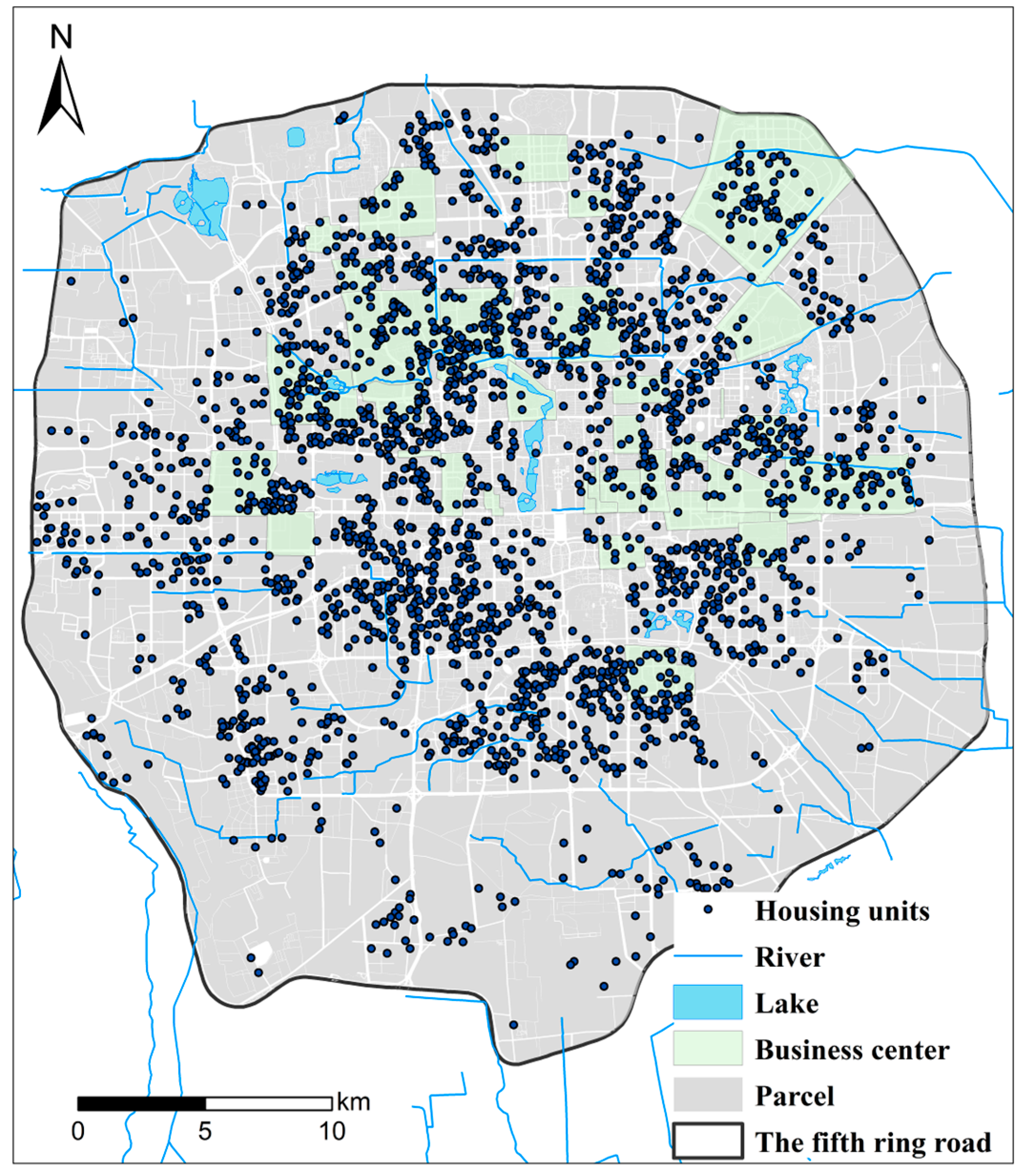
2.1. Study Area

In 2014, the fifth ring road area in Beijing, China, was approximately 669 km2, which accounted for 4.1% of the area of Beijing city. However, the population in this area was approximately 10.5 million people, which accounted for 48.4% of the total population of Beijing. Thus, the fifth ring road area is the main centre in Beijing. A map of the whole study area and the geographic elements are shown in Figure 1. There were 6103 road segments with a cumulative length of 1925.1 km. There were 33 main business districts located in the study area, with an average acreage of 5.1 km2. Some famous business districts, such as Dongdan, Xidan, Wangfujing, and Wudaokou, had concentrated commercial facilities and a good ability to attract industry. The fifth ring road area of Beijing is a typical and meaningful study area, so many studies have been conducted here [2,26,42,43,44].

2.2. Data Acquisition

The basic geographical data we used in the study were electronic navigation map data from Autonavi, generated in 2014 and covering parks, schools, and bus and metro station POIs (points of interest) in addition to roads, rivers, lakes, and business district polygon shapefiles. The parcel data were for the year 2012, so there was some mismatch with 2014’s Autonavi data, especially in the street network. We used these street data only for better map visualization so that this would not influence our results.
The HGVI values were calculated based on massive Tencent street view image datasets from 2014, and SegNet [45]. To decrease the influence of seasonal change, we used street view images taken from April to October in 2014. The street view samples were selected by sampling along the road centreline at 100 m intervals, and at road intersections. Every sample point was represented by six street view images with an intersection angle of 60 degrees. A total of 208,746 street view images were obtained using the Tencent static picture API. For more detail on the crawling technique, see [34,46]. The massive street view image dataset that we developed was adopted as a surrogate of urban streetscapes in Beijing, and was used to perform further analysis over a large geographical area and to develop new metrics for the hedonic pricing model in the study.
The housing transactions and basic housing characteristics data were obtained from the Fang Company, which is a large global real estate platform covering transactions information from 642 cities all over the world (www.fang.com). The data included 22,331 transaction records in the study area in 2014 (excluding 152 invalid or omitted records). The main fields in the transaction records were the name of the residential development, housing area, window orientation, transaction price, the age of the residential development, address, geographical coordinates, building types, residential unit housing number, households, plot ratio, green coverage rate, and residential unit building number. Since most residential units had multiple transaction records (the average number of records was 9), these transactions were aggregated by residential unit, and we obtained 2370 transactions at the housing estate level for further analysis.
The statistical analysis software adopted in the article was Stata 14, which was mainly used for building regression models and statistical analysis. The crawler for obtaining the Tencent street view images and batch processing applications for the massive image datasets was written in Python, and the maps were produced in ArcGIS 10.2. The shortest distances between housing units and the amenities along the road network were calculated using the Network Analyst models of ArcGIS.

3. Methods

3.1. Hedonic Pricing Model

Hedonic pricing models have different forms; for example, linear models [47], semi-log models [48,49], and double-log models [23]. Generally, it is difficult to confirm whether one has an absolute advantage over the others [50], but this could be determined through experimental examination [11,51] or research [52]. Among the model forms, the semi-log model has five overall advantages: first, this model considers the variation of each independent variable; second, it is relatively easy to explain the implied values of the independent variables; third, this form can reduce the heteroscedasticity in the model; fourth, the calculation of this approach is simple; and fifth, this approach produces a flexible model [53]. In summary, based on the advantages above, we decided to build a semi-log hedonic pricing model with log-dependent variables and a linear combination of independent variables, the mathematical equation of which is shown in Equation (1). The estimates of this semi-log hedonic model can imply the percentage change in housing prices as a response to a unit change in an independent variable:
ln P = α 0 + β τ C τ + ln H G V I + ε
In Equation (1), P is the average transaction price at the residential unit level; lnP is the logarithmic form of P; β τ is the coefficient of a housing characteristic ( τ [ 1 ,   2 ,   3 , ,   24 ] ); ln H G V I is the logarithm form of HGVI; α 0 is the intercept term; and ε is the error term. The descriptions and statistics for the 25 characteristic variables in the model are illustrated in Table 1. The dependent variable LSPRICE is P in Equation (1).
Our hedonic model included three categories of characteristics; namely, location, housing, and neighbourhood characteristics. We took BC_DIS and C_DIS, which represent the shortest road distance from the housing unit points to business centres and the city centre (Tiananmen Square) of the study area, respectively, to reflect the location characteristic of housing prices. A detailed description of BC_DIS and C_DIS is shown in Table 1. All accessibility variables were calculated by road network distance in the article. Additionally, the 0.5 km and 1 km distance buffers were calculated by road network distance.
The housing characteristics included the following variables: AREA, YEAR, HS, PR, PF, and GR and the dummy variables ORI, TOWER, and SLAB. For ORI, if the residence has north-facing windows, the value is 1; otherwise, the value is 0. TOWER and SLAB are dummy variables. If the building type is a tower, the TOWER variable is 1; if the building type is a slab, the SLAB variable is 1; otherwise, the two variables are 0.
Concerning the neighbourhood characteristics, the variables measuring the accessibility to bus stations, metro stations, and schools (including kindergartens, primary schools, junior middle schools, senior high schools, and colleges) along road networks were included in our hedonic model (BUS_DIS, SUB_DIS, and SCH_DIS). We took the means of road network metrics to measure the length along roads between housing units and urban amenities in order to obtain a realistic result. In addition, we added the number of bus stations and schools within 0.5 km and 1 km road distances into the model (0.5 km: BUS_5H, SUB_5H, and SCH_5H; 1 km: BUS_1T, SUB_1T, and SCH_1T). As indicated by the statistics in Table 1, the densities of bus stations, metro stations, and schools could have an impact on housing prices, since the concentration of amenities can have an impact on the housing prices of residential units [26]. Except for the traffic and educational aspects, several independent variables were used to measure and explain several natural or semi-natural amenities, including PARK_DIS, LAKE_DIS, LAKE_AREA, RIVER_DIS, and HGVI. The definitions and equations for HGVI will be illustrated in the next two sections.

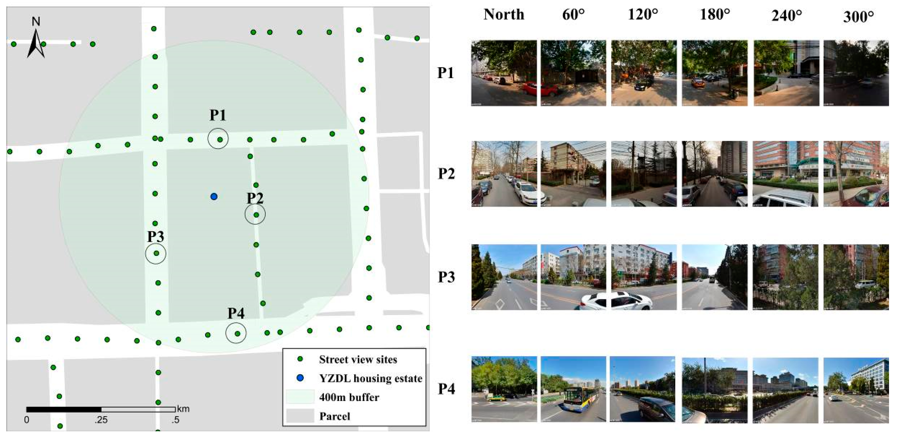
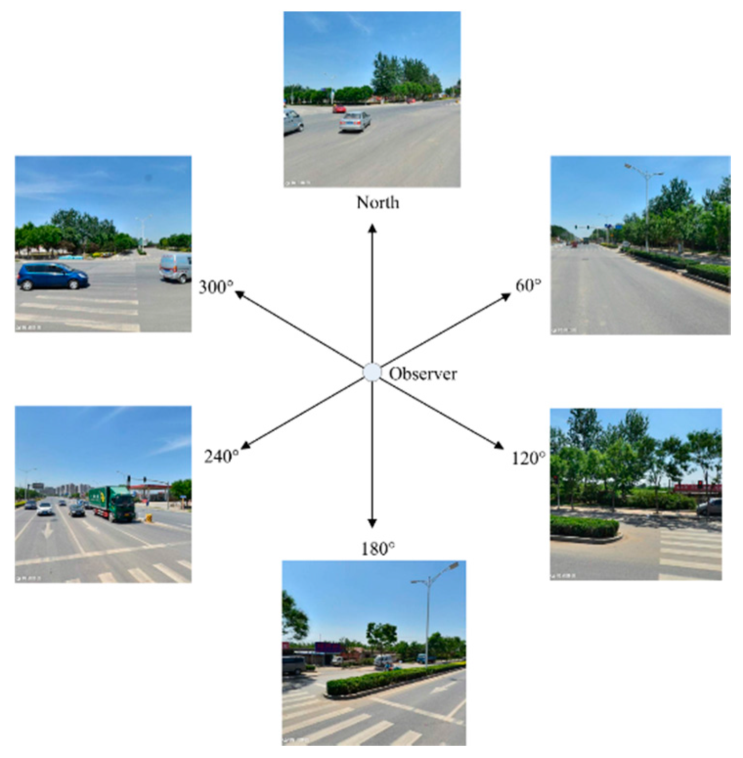
3.2. Equation of the Horizontal Green View Index

The calculation equation for the GVI is closely related to the configuration and arrangement of street view images and scene photos. Yang et al. [33] first used scene photos at road intersections to calculate the GVI value. On the basis of Yang et al.’s [33] study, Li et al. [34] used eighteen Google street view images and modified the GVI equation. Then, Long and Liu [38] used four Tencent street view images facing north, east, south, and west to calculate the GVI with an image resolution of 960 × 480. In this article, we simplified Li et al.’s [34] calculation equation and took six horizontal Tencent street view images with 600 × 600 resolutions and an intersection angle of 60 degrees to represent the streetscapes (see Figure 2). Our simplified indicator is called the HGVI in this study to differentiate from those used in other studies. Using Equation (2), we can obtain the HGVI values at all street view sample sites in Beijing:
H G V I = A r e a green A r e a total × 100 %

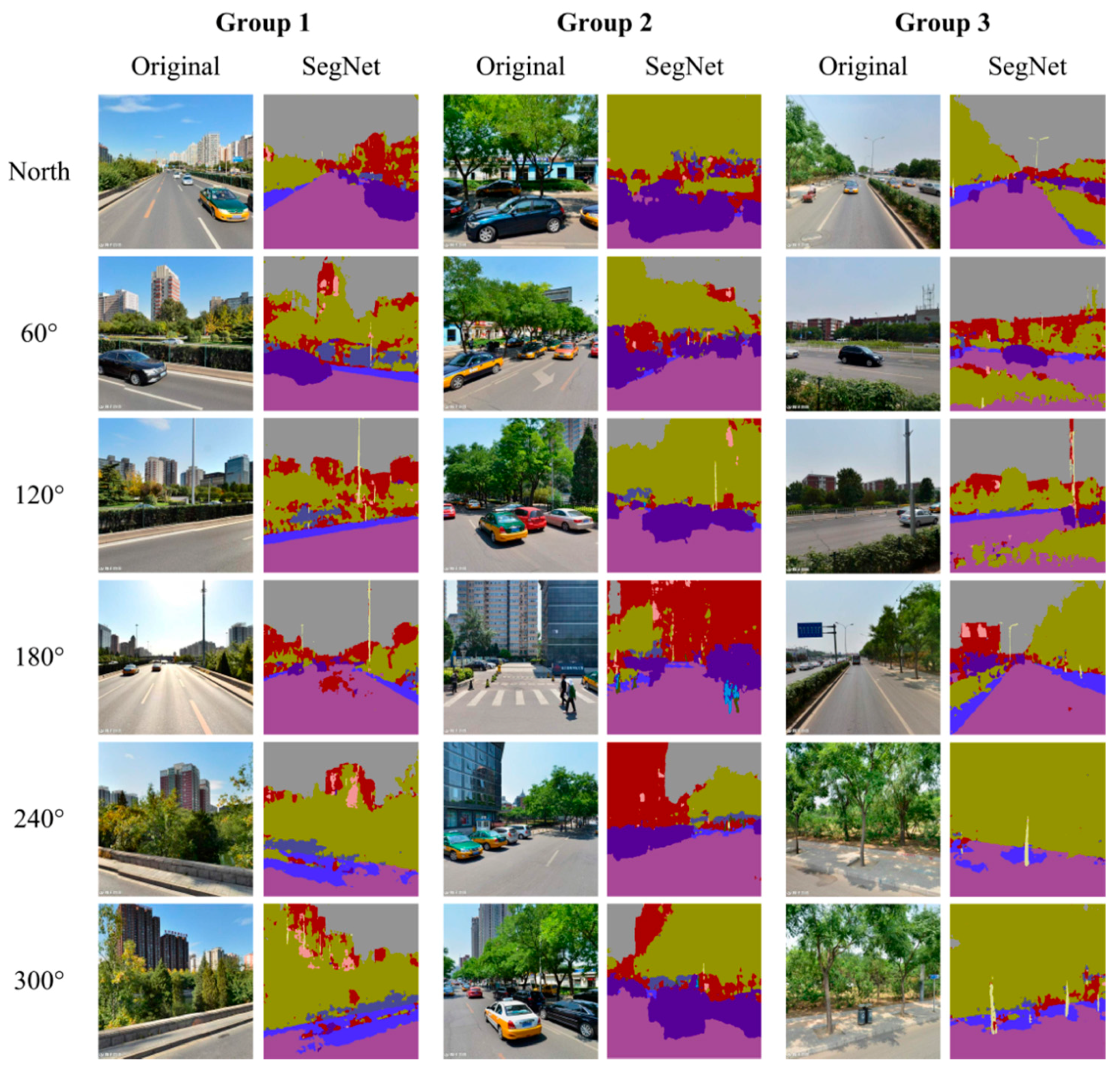
3.3. Calculating HGVI Based on SegNet
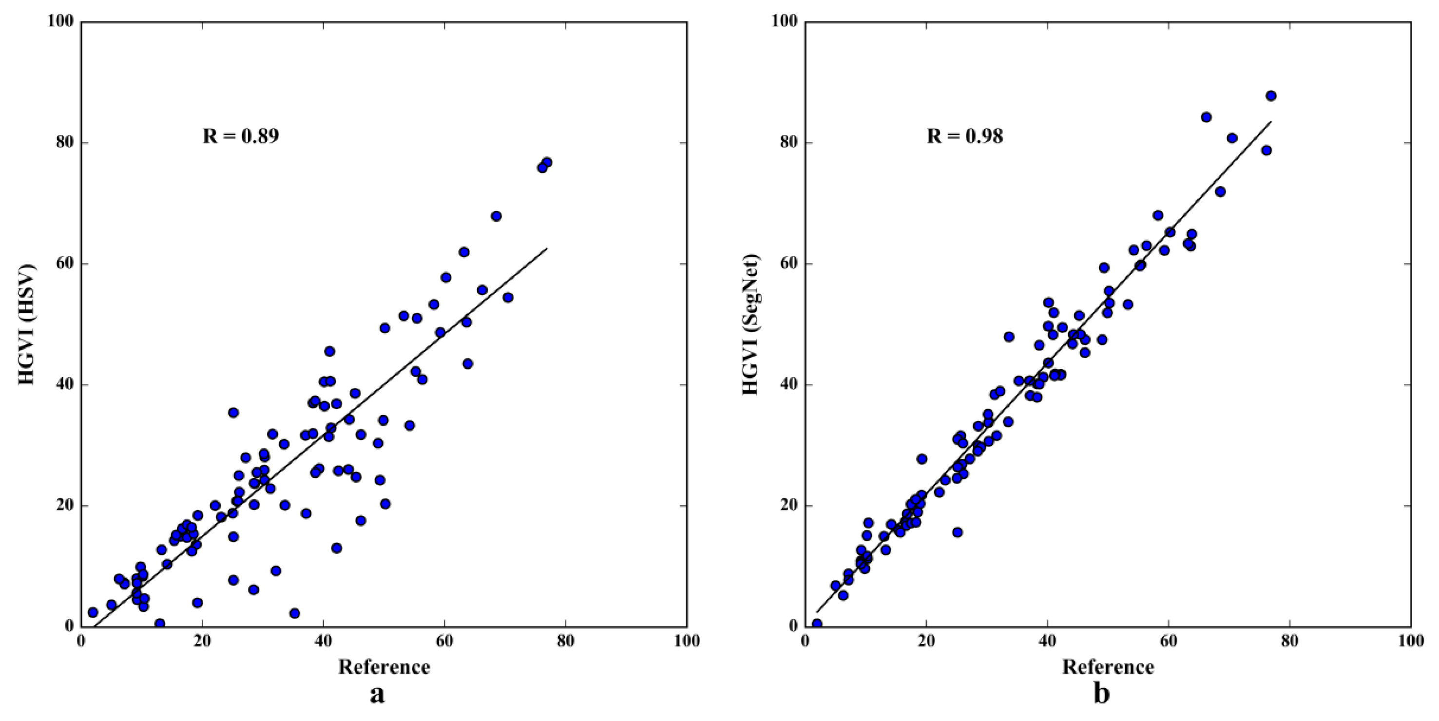
We adopted SegNet [45], which is a pixel-level semantic segmentation method, to quantify the green vegetation information from the crawled street view images. At the core of SegNet is a deep convolutional neural network encoder-decoder architecture [45], which can be used for recognising and extracting multiple landscape elements, such as green vegetation, sky, cars, pedestrians, fences, and buildings from RGB (red, green, and blue channels) pictures. In this study, we trained the deep convolutional neural network (DCNN) based on a GPU-accelerated mode (graphics processing unit) using the CamVid dataset (a driving photo dataset) [54] and iterated 5 million times so that the accuracy for the training data reached over 99%. The configuration of the hardware devices used in the experiment was one NVDIA TITAN Xp graphics card with 12 GB of video memory and 64 GB of physical memory, and an Intel Xeon E5-2630 CPU (central processing unit). The operation system of the computer was 64-bit Ubuntu 16.04.2 LTS. Finally, we used the trained DCNN model to patch the 208,746 street view images together and further calculated the HGVI values based on Equation (2).
To verify the accuracy of the segmentation results, we compared the HGVI results of SegNet and the artificial segmentation results of Photoshop using linear regression. This method uses the artificial segmentation results from Photoshop as a reference, and if the regression result was significant and the coefficient was high, the results were accurate. In addition, we also built a regression model between the results of the HSV colour model and the references for comparison of the regression model with SegNet and the references. The details of this verification step are shown in Section 3.4.
In this paragraph, we illustrate the HGVI calculation for a residential unit. Taking the YZDL community as an example, the HGVI of all street view sites with a 400 m radius circle buffer was averaged, and this mean value was the HGVI value at the residential unit level, representing the perception of street greenery neighbouring the residential unit (see the left sub-picture in Figure 3). The buffer radius was defined based on our experiences and analysis. The buffer should cover the streets neighbouring the residential units as much as possible. Additionally, the normal radius of residents’ activities should be taken into account. The radius capturing the activities of most American people is approximately 200 m from the home [55]. However, the basic dwelling unit in China was the housing unit, and there is a large difference between the residential conditions and traditions in China as compared to America (see Jiao and Liu [56]). Therefore, we took the approximate square root value (approximately 400 m) as the radius for HGVI calculation based on the mean acreage (419.5 m2) of residential units in Beijing. After calculating the HGVI values of all residential units in study area, there were approximately 36 street view sites neighbouring a residential unit, and the residential units with three sample sites or less were excluded from our study. Each street view site on the roads in Beijing was related to a set of Tencent street view pictures, and the configuration and arrangement of these images have been shown previously in Figure 2. Four example points (P1 to P4) in the right sub-picture in Figure 3 show the corresponding street view images.

3.4. Verifying HGVI

To observe the segmentation effect, we randomly took three groups of street view images from the dataset, and each group included the original street view image and the SegNet result (see Figure 4). The polygons labelled in green are the visible greenery segmented by SegNet. The HGVI value for each street view site was easily calculated.
To verify the accuracy of the segmentation process, we randomly selected 100 street view images from the image database and used the HSV colour model [38], SegNet [45], and artificial segmentation with Photoshop [33] to calculate the proportions of greenery in each image. Two linear regression models were built; namely, one between the HSV colour model results and the references and another between the SegNet results and the references. The regression verification indicated that the Pearson’s coefficient of the first model was 0.89; in contrast, the coefficient of the second model was 0.98, which was relatively higher (see Figure 5a,b). Moreover, from Figure 5b we can see that the fitting line is closer to the diagonal line of the graph than the fitting line in Figure 5a. In summary, using SegNet to calculate the HGVI values with street view images was accurate and feasible.

4. Results

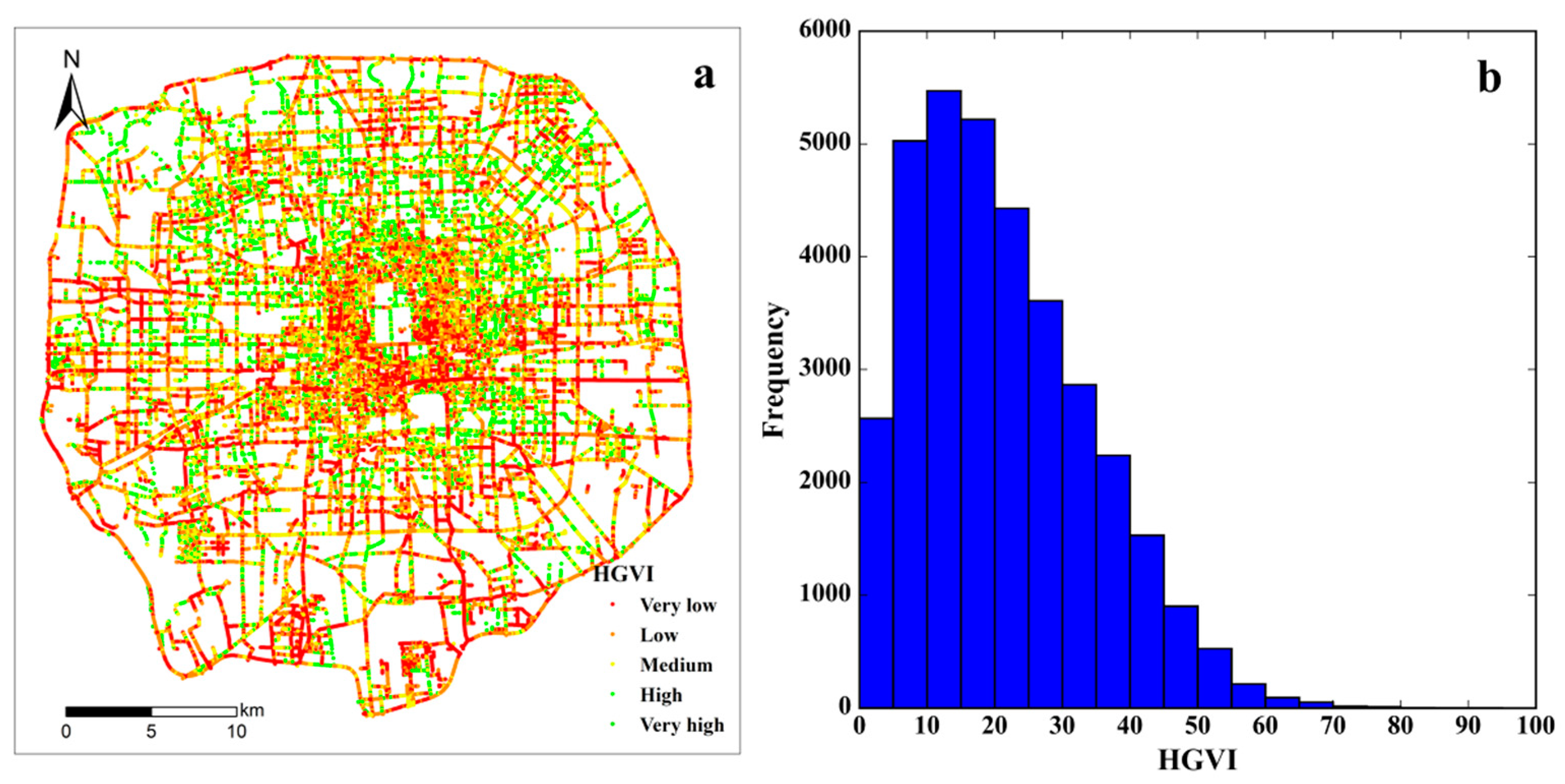
4.1. Distribution of HGVI in the Study Area

As in the method mentioned above, all the HGVI values at street level in the study area can be calculated based on the HGVI equation and SegNet. The HGVI values were classified into five classes by the natural breaks method: very low (0.16, 11.30), low (11.31, 20.51), medium (20.52, 30.66), high (30.67, 43.06), and very high (43.07, 90.03). The street-level HGVI map in Figure 6a showed that the street-visible greenery in the northern region of the study area was higher than that in the south. The map also showed that the street network in central Beijing was denser than that on the periphery, and HGVI values of the street view sites at low and very low levels dominated in this area. The average and standard deviation of all of the HGVI data at street level were 21.3 and 13.0, respectively, and the HGVI data exhibited an approximately log-normal distribution, thus, a logarithm transformation for the HGVI variable was necessary in the hedonic pricing model.

4.2. OLS Regression Results

We used the “reg” command in Stata 14 to build the ordinary least squares (OLS) regression model and added the additional term “robust” into the model to make the standard error more robust and reduce the effect of heteroscedasticity on the regression results; for more details, see Stock and Watson [57]. The OLS regression results of the two models are shown in Table 2. Model 1 shows the full-variables hedonic model and Model 2 shows the hedonic model excluding non-significant variables. The percentage of total variation explained by our model reached about 75.4% (Model 1 and 2’s R2 values were very close). In examining the coefficients of the characteristic variables in the model, all location characteristics, including BC_DIS and C_DIS, were clearly highly significant in the model. Most of the housing characteristics in the model were significant, including AREA, YEAR, PR, PF, GR, and TOWER. Most of the neighbourhood characteristics, including BUS_5H, BUS_1T, SUB_DIS, SUB_5H, SUB_1T, SCH_DIS, SCH_1T, LAKE_AREA, and the newly-developed HGVI, were significant in the model. Comparing the two models in Table 2, the significance of the variables YEAR, BUS_5H, and SUB_DIS in Model 2 increased. The coefficients of the significant variables demonstrated a very small change. The marginal prices of the characteristics (except HGVI) in the model were obtained by multiplying the non-standardized coefficients of those characteristics by the mean housing prices at the residential unit level (RMB 3,429,300). The percentage change in HGVI was calculated based on the formula 2 b 1 , where b is the non-standardized coefficient of HGVI, since it is in logarithm form.
To test for the multicollinearity effect in the model, we used VIF (variance inflation factor) to check all of the model parameters. All the VIFs of the independent variables were lower than five, which indicated that those variables did not have serious multicollinearity. The VIFs in Model 2 were smaller than in Model 1 for each variable except YEAR. In addition, the Durbin-Watson test results of Model 1 and 2 were 1.66 and 1.65, separately; these were both close to two, meaning that the autocorrelations in the models are weak. On the basis of the models in Table 2, we finally decided to use Model 2’s coefficients to estimate the marginal values of characteristics for the purpose of obtaining a fine value estimate.

4.3. The Regression Results for Location Characteristics

For every 1 km decrease in the distance between business centres and the housing unit (BC_DIS), the housing price increased by 3.1% (RMB 106,308). The C_DIS variable was relatively weaker, and a similar decrease in distance increased the housing price by 1.6% on average (RMB 54,869).

4.4. The Regression Results for Housing Characteristics

The AREA variable is the dominant factor in the model (t-value = 34.8). When AREA increased by 1 m2, the housing price increased on average by 1% (RMB 34,293). YEAR has a negative effect on housing prices, and a one-unit increase can decrease housing prices by 0.12% (RMB 4115) on average. PR is significant at the 10% level in the model, and a one-unit increase can decrease housing prices by 0.65% (RMB 22,290). When PF increases 1 RMB per m2 per month, the relative housing price increases by 2.2% (RMB 75,445), on average. GR reflects the greenery coverage inside the residential unit, and a 1-unit increase can improve the housing price by 0.1% (RMB 3429) on average. SLAB and TOWER are dummy variables (the percentage change in dummy variables is calculated based on the formula e b 1 , where b is the non-standardized coefficient and e is the natural base of the logarithm). The TOWER variable is highly significant at the 1% level. Compared to other building types, a one-unit increase in this variable can decrease the housing price by 7.1% (RMB 243,480) on average. Other variables, such as SLAB, ORI, and HS, are not statistically significant in the model.

4.5. The Regression Results for Neighbourhood Characteristics

The independent variables BUS_DIS and SCH_5H are not statistically significant in the first model. However, BUS_5H, BUS_1T, SUB_5H, SUB_1T, and SCH_1T are statistically significant at the 1% level. SUB_DIS and SCH_DIS are significant at 5% level. Among these variables, a one-unit increase in BUS_5H and BUS_1T can decrease housing prices by 0.18% (RMB 6173) and 0.1% (RMB 3429) on average, which indicated that the concentration of bus stops within a 0.5 km or 1 km radius has a slightly negative effect on housing prices. For SUB_1T and SCH_1T every one-unit increase can increase housing prices by 1% and 0.2% (RMB 34,293 and 6859), respectively, on average. However, the estimate of SUB_5H shows it can decrease the housing price by 0.76% (RMB 26,062). The significant road distance variables SUB_DIS and SCH_DIS have a different status; SUB_DIS can decrease the housing price by 1.1% (RMB 37,722), while SCH_DIS can increase the value by 4.1% (RMB 140,601), on average.
In our hedonic model, PARK_DIS, LAKE_DIS, LAKE_AREA, RIVER_DIS, and HGVI are variables that reflect the characteristics of neighbouring natural or semi-natural landscapes. First, PARK_DIS, LAKE_DIS, and RIVER_DIS are all not significant in the first model, which implies that the road distance from housing units to parks, lakes, and rivers in Beijing does not have a significant effect on housing prices based on our data. Second, LAKE_AREA has significant positive impact on housing price, and a one-unit increase in this variable can increase housing prices by 17% (RMB 582,981) on average. This result implies that lake area is a powerful characteristic in our model. Finally, according to the HGVI_LN in the model, the variable of residential developments has a significant and positive impact on housing prices at the 1% level, and a one-unit increase can increase the residential estate value by 10% (RMB 342,930) on average, which means an improvement in HGVI can significantly increase the nearby housing prices.

5. Discussion

In this section, we further discuss the characteristic elements, such as location, housing, green landscape, other landscape, traffic, and educational facilities to analyse their impacts on Beijing’s housing prices at the residential unit level. Then, we summarize the advantages of methods combining computer vision with massive street view image datasets. Following this, several recommendations are presented for domestic decision-making and urban planning. Finally, limitations and future research directions are presented.

5.1. Impact of Location Characteristics on Housing Prices

Many studies have shown that the distance from housing units to the city centre and sub-centres can affect housing prices. Our results demonstrated that BC_DIS and C_DIS have negative relationships with housing values. The result for C_DIS was consistent with that found by Yang [58], Jim and Chen [22], Shin, et al. [59], and Chen and Hao [60], but was inconsistent with that in the studies by Mcleod [61], Bae, et al. [62], and Jiao and Liu [56]. In Wuhan city, China, Jiao and Liu [56] found that the distance to the city centre did not have a significant impact on Wuhan’s housing prices because Wuhan is a polycentric city. Yang [58] demonstrated that a shorter distance from residential developments to the city centre has a significant and positive impact on housing prices in Beijing. In contrast, Xiao et al. [26] indicated that a shorter distance from houses to city sub-centres increases Beijing’s real estate values. These two studies did not indicate whether the two distances impact Beijing’s housing prices simultaneously. Multiple urban sub-centres can produce heterogeneous pulling effects that simultaneously compete with and supply conventional city centres [63]. In our model, BC_DIS and C_DIS both had significant and negative correlations with Beijing’s housing prices, and the hedonic models did not have clear multicollinearity or autocorrelation, indicating that Beijing’s housing prices were affected by BC_DIS and C_DIS simultaneously. This result occurs because the early spatial development of Beijing (before the 1990s) was focused on expanding around the city centre, but after the inner built-up area was saturated, the external expansion model evolved toward multi-centre development with a fast urbanization process. Therefore, the real estate prices were affected by the complex spatial model around the city centre and business centres (sub-centres). In other words, present-day Beijing has a monocentric and polycentric compounded spatial pattern.

5.2. Impact of Housing Characteristics on Housing Prices

AREA is a dominant independent variable in our model, which is consistent with the findings of several studies in Guangzhou [22,49], Shenzhen [12], and Beijing [12] in China, and in some western cities [21,23]. The coefficient of PF indicated that Beijing’s homebuyers would be willing to pay for resident units with better community property services. The willingness for homebuyers to maintain a high-quality living experience translates into a willingness to pay for this experience. YEAR is a significant and negative characteristic in the model and represents the age of the residential unit. This finding is consistent with those of studies in Shenzhen [64] and Beijing [26]. For housing unit building types in Beijing, the data showed that compared to slab and other building types, homebuyers dislike tower buildings. In addition, the coefficient of PR indicated that people do not like to live in an intensively residential environment.

5.3. Impact of Green Landscapes on Housing Prices

Previous literature has indicated that tree canopy cover can have positive impacts on neighbouring housing prices [29,30,31,65]. However, because street greenery was described in different ways in these papers, tree cover cannot fully represent what people truly perceived. A study in Hong Kong indicated that street views could have negative impacts on housing price [24]. However, the study did not indicate which specific street view element had negative impacts. Streetscapes are heterogeneous and complex, and are composed of multiple visual elements. In our study, we used a computer vision method to analyse massive street view image datasets to measure the greenery visible on Beijing’s streetscapes. Additionally, we built a hedonic pricing model to establish a quantitative and economic relationship between street-visible greenery and real estate values.
The coefficient of HGVI in the model shows that the HGVI of residential units has a significant and positive relationship with housing prices and, thus, a core conclusion can be obtained: Beijing’s homebuyers would be willing to pay a premium for houses in residential units with higher HGVI values. This finding indicates that homebuyers in Beijing prefer to see more greenery around residential developments. GR is a frequently used indicator that measures the green coverage in a residential unit in China. This indicator has been shown to have a positive impact on housing prices in Wuhan, China [56], and the coefficient of GR in our model aligns with this result. Therefore, housing prices are affected not only by green coverage inside the residential units, but also by neighbouring street-visible greenery. Comparing both the coefficients of HGVI and GR in the model, the marginal price of HGVI is much larger than that of GR. The visible greenery neighbouring residential units has a positive effect on housing prices and this impact is strong (10%). Therefore, improvements in street-visible greenery could cause very large increases to housing prices in Beijing, which would also increase the revenues for housing developers, investors, and real estate agencies. In recent years, Beijing’s government has been working on the construction of open blocks. The outer walls of many gated communities have been changed to perspective fences or have even had fences removed. In these projects, the impacts of street-visible greenery on the housing prices would be greater. To summarize, Beijing’s government should encourage vertical greening and ensure the visibility of the street greenery around residential units. These approaches can satisfy the consumption demands of homebuyers and will improve the aesthetic values of urban streets.
Our results indicate that homebuyers have actual requirements for street-visible greenery neighbouring residential units. When house buyers are going to buy a house, they usually investigate and compare housing information through the Internet, real estate trade magazines, or newspapers. If they really want to buy the house, they go to the residential units to see the houses and housing environments because buying a house is an important decision for most Chinese people. In addition, most of the residential units in Beijing are gated, have security guards, and are surrounded by walls. Thus, before the buyers go into the residential unit, the first scenes they will see are the streetscapes and neighbouring street greenery. The quality of the exterior scene and streetscapes may provide a first impression to homebuyers. However, because of the different preferences of different people, this impression may be positive or negative. For instance, if the buyers see poor street views with very little greenery surrounding the residential unit, their intention to buy may decrease. However, if they see high-quality surrounding streetscapes, their intention to buy may be strengthened. In addition, residents are commonly active in the areas neighbouring the residential unit and in the unit itself. Old and retired persons may take walks or walk their dogs near their residential unit to enjoy their lives in peace and safety because of the close proximity to their homes and the perceived safety of their environment. Residents may go to supermarkets and restaurants close to their houses, and during their walk, they can view the street greenery, which is important and easily overlooked. In summary, most of Beijing’s homebuyers may unconsciously form a willingness to buy a house with abundant street greenery neighbouring the community.

5.4. Impact of Other Landscapes on Housing Prices

While HGVI and GR represent the green environment of residential units, several other metrics, such as PARK_DIS, LAKE_DIS, LAKE_AREA, and RIVER_DIS, measure other urban landscape characteristics. The results show that Beijing’s homebuyers have non-significant preferences for buying houses close to parks, which is inconsistent with the results of Luttik [66] and Pearson, et al. [67]. This could be caused by the excessive utilisation of parks by many people, resulting in the production of a large amount of noise and other environmental stresses that reduce the living quality of the surrounding residents.
With regards to urban water bodies, based on the coefficients of LAKE_AREA and LAKE_DIS, we find that Beijing’s buyers favour lakes with larger areas however they have not shown a preference for the road distance to them. In other words, the road distance to lakes is not a significant characteristic. This finding occurs because the water bodies in Beijing have been seriously polluted [68,69], which can decrease the ecological effects and aesthetic values of lakes. The negative correlation between water bodies and housing prices has been demonstrated in several studies (e.g., Huang and Yin [17], Luttik [66]). Similarly, the distance to rivers in our model is also not a significant characteristic, which may also be due to river pollution. Therefore, regulators and the public should take actions to protect the rivers and lakes in Beijing in order to improve water quality.

5.5. Impact of Traffic and Educational Facilities on Housing Prices

Our results demonstrate that the road distance to the nearest bus stations does not significantly affect housing prices. The density of bus stations within a 0.5 or 1 km radius of the residential unit has a negative impact on housing prices. This is because bus stations may cause noise pollution. The road distance to metro stations has a negative impact on nearby housing prices because metro lines are very convenient and fast transportation for residents in their daily lives. The number of metro stations within 0.5 km road distance has a negative impact on housing prices. This is because homebuyers would not like their living environment to have too many metro stations nearby. However, increasing the number of metro stations within a 1 km road distance would have a positive impact on surrounding housing estates. This indicates that the metro stations concentrated within a 1 km road distance can provide a desirable traffic service to local residents. This finding could be a reference for metro station planning and arrangement. The density of educational facilities within 1 km could raise housing prices, which suggests that buyers tend to pay a premium for residential units surrounded by more schools. Such a configuration could give parents more schools to choose from for their children [70]. However, our data shows that the road distance to schools has a positive impact on housing prices, which means homebuyers do not prefer their houses to be very close to schools. This finding occurs because our school POI data includes many different types of education institutions. Further studies could discuss whether the types of schools in Beijing have an impact on housing prices.

5.6. The Advantages of Using Street View Images and Computer Vision

Using street view images could enable urban studies to be conducted on a large scale. Street view pictures have advantages that remote sensing images lack. These pictures can reflect the visual perceptions of people to some extent, and can enable policy-makers and planners to understand urban streetscapes and their elements from the perspective of the public [34,71]. Compared to questionnaires, field investigations [12], and Earth observation studies [72], using street view images and computer vision techniques has several advantages [39]. First, these approaches reduce human interference, while questionnaires need to consider gender, educational level, age, and other factors related to both the respondents and the investigators, all of which can influence the experimental results. Second, this method has advantages in data coverage and size. Third, this method can significantly reduce labour and save time because most of the procedures are completed with Python scripts. Fourth, street view images could be suitable supplements to remote sensing images for the vertical dimension, and have a high resolution for streetscape studies [37]. Finally, street view images represent low-cost datasets for researchers compared with high-resolution remote sensing images.

5.7. Policy Guidance and Recommendations

Our empirical results indicate that street-visible greenery neighbouring residential units in Beijing increased housing prices. Housing developers have obtained benefits from the surrounding street greenery but have not provided support or assistance for street greening. Therefore, the Beijing Municipal Government could levy a “green value tax” specifically on property developers. The urban landscaping department could establish a standard HGVI range (the agreeable street-visible greenery range). The specific tax amount could be calculated according to our method if the HGVI value of a residential unit is within the range. Such a measure could increase the funding for subsequent public environmental optimization and development. Additionally, such a measure will bring property developers, managers, and owners to the forefront of public street greening, especially for streets close to residential units. This research could broaden the horizon of policy-makers, i.e., enabling them to not merely focus on the tree coverage inside or outside the residential units, but also on how much greenery residents, pedestrians, and homebuyers can actually see. HGVI could represent a new metric and quantification method for street greenery planning and could be employed as a characteristic in property evaluation. During future urban street greenery planning and design, the planner should pay attention to the visible greenery within the line of sight and give pedestrians and drivers enough visible greenery to view, which can provide improved landscape aesthetics during their activities and meet the demands of most home buyers in residential environments.

5.8. Limitations and Future Research

As we were limited by the acquisition of residential unit shapefiles, we neglected the topology of the polygons of residential units, which could cause some bias. In future studies, a “donut” buffer could be employed when calculating the HGVI value of residential units. Our study used only cross-sectional data from the year 2014, so further studies could be conducted to add time dummy variables to analyse the temporal dynamics of housing prices in a hedonic pricing model. SegNet can also quantify other visual elements of streetscapes, and those elements could be incorporated into hedonic pricing models to explore their impacts on housing prices. Spatial econometrics models could be used in future research to further improve the accuracy of the model.

6. Conclusions

We analysed three categories of major characteristics of housing prices; namely, location, housing, and neighbourhood characteristics, based on a hedonic pricing model. First, we introduced the HGVI as an indicator measuring the street-visible greenery neighbouring residential units and explored its impacts on housing price. From this empirical study, several key conclusions can be drawn. First, the street-visible greenery neighbouring properties has a positive relationship with property values. This finding indicated that Beijing’s buyers are willing to pay a premium for houses with higher HGVI values, a finding that has not been discussed in previous studies. Second, we found that Beijing’s homebuyers do not like to live close to lakes, but favour lakes with larger areas. This result could be caused by the heavy pollution of such water bodies. Third, location characteristics, including the shortest distance to the city centre and business centres, had powerful impacts on housing prices. This finding indicated that Beijing’s housing prices were driven by the development mode of the city centre and sub-centres.
We provided a new empirical study for Beijing city that combined street visual perception and housing transactions. Our results demonstrated that buyers were willing to pay for adequate street-visible greenery neighbouring residential units. This article offers a tool for quantifying and analysing the street-visible greenery surrounding gated residential units. Planners and policy-makers should pay attention to the layout and design of vertical greening (e.g., green roofs and walls) in residential environments because the economic values of these structures have often been neglected. This study can help property developers realize and understand the demands of the real estate market and develop elegant and agreeable residential products. In addition, the HGVI map could serve as a reference for the allocation of greening resources. In further studies, our method could be applied to other megacities in China to verify the feasibility of the method and the universality of our conclusions.
Using massive street view picture datasets and computer vision quantification offers some advantages for urban streetscape studies. Our quantification method and the HGVI indicator, which were used to quantify the visual elements of streetscapes, could supplement real estate studies that use the hedonic pricing method. Most of the calculations were completed by Python scripts, which improved the efficiency.

Acknowledgments

This study was funded by the National Key Research and Development Program Grant (2016YFC0503605).

Author Contributions

Rencai Dong and Yonglin Zhang conceived and designed the experiments; Yonglin Zhang performed the experiments; Yonglin Zhang analysed the data; Yonglin Zhang contributed the analysis tools; Rencai Dong and Yonglin Zhang wrote the paper; and all the authors reviewed and edited the manuscript.

Conflicts of Interest

The authors declare no conflict of interest.

References

  1. Wu, J. Urban ecology and sustainability: The state-of-the-science and future directions. Landsc. Urban Plan. 2014, 125, 209–221. [Google Scholar] [CrossRef]
  2. Qian, Y.; Zhou, W.; Yu, W.; Pickett, S.T.A. Quantifying spatiotemporal pattern of urban greenspace: New insights from high resolution data. Landsc. Ecology 2015, 30, 1165–1173. [Google Scholar] [CrossRef]
  3. Asgarzadeh, M.; Koga, T.; Hirate, K.; Farvid, M.; Lusk, A. Investigating oppressiveness and spaciousness in relation to building, trees, sky and ground surface: A study in Tokyo. Landsc. Urban Plan. 2014, 131, 36–41. [Google Scholar] [CrossRef]
  4. Asgarzadeh, M.; Lusk, A.; Koga, T.; Hirate, K. Measuring oppressiveness of streetscapes. Landsc. Urban Plan. 2012, 107, 1–11. [Google Scholar] [CrossRef]
  5. Ulrich, R. View through a window may influence recovery from surgery. Science 1984, 224, 420–421. [Google Scholar] [CrossRef] [PubMed]
  6. Takano, T.; Nakamura, K.; Watanabe, M. Urban residential environments and senior citizens’ longevity in megacity areas: The importance of walkable green spaces. J. Epidemiol. Community Health 2002, 56, 913–918. [Google Scholar] [CrossRef] [PubMed]
  7. Ben-Joseph, E.; Lee, J.S.; Cromley, E.K.; Laden, F.; Troped, P.J. Virtual and actual: Relative accuracy of on-site and web-based instruments in auditing the environment for physical activity. Health Place 2013, 19, 138–150. [Google Scholar] [CrossRef] [PubMed]
  8. Hillsdon, M.; Panter, J.; Foster, C.; Jones, A. The relationship between access and quality of urban green space with population physical activity. Public Health 2006, 120, 1127–1132. [Google Scholar] [CrossRef] [PubMed]
  9. Richardson, E.A.; Pearce, J.; Mitchell, R.; Kingham, S. Role of physical activity in the relationship between urban green space and health. Public Health 2013, 127, 318. [Google Scholar] [CrossRef] [PubMed] [Green Version]
  10. Rosen, S. Hedonic Prices and Implicit Markets: Product Differentiation in Pure Competition. J. Political Econ. 1974, 82, 34–55. [Google Scholar] [CrossRef]
  11. Palmquist, R.B. Estimating the Demand for the Characteristics of Housing. Rev. Econ. Stat. 1984, 66, 394–404. [Google Scholar] [CrossRef]
  12. Chen, W.Y.; Jim, C.Y. Amenities and disamenities: A hedonic analysis of the heterogeneous urban landscape in Shenzhen (China). Geogr. J. 2010, 176, 227–240. [Google Scholar] [CrossRef]
  13. Hanushek, E.; Yilmaz, K. The complementarity of Tiebout and Alonso. J. Hous. Econ. 2007, 16, 243–261. [Google Scholar] [CrossRef]
  14. Hanushek, E.A.; Yilmaz, K. Household Location and Schools in Metropolitan Areas with Heterogeneous Suburbs; Tiebout, Alonso, and Government Policy. NBER Working Paper No. 15915. Soc. Sci. Electron. Publ. 2010, 40, 102–106. [Google Scholar]
  15. Hanushek, E.A.; Yilmaz, K. Schools and Location: Tiebout, Alonso, and Governmental Finance Policy. J. Public Econ. Theory 2013, 15, 829–855. [Google Scholar] [CrossRef]
  16. Powe, N.A.; Garrod, G.D.; Willis, K.G. Valuation of urban amenities using an hedonic price model. J. Prop. Res. 1995, 12, 137–147. [Google Scholar]
  17. Huang, H.; Yin, L. Creating sustainable urban built environments: An application of hedonic house price models in Wuhan, China. J. Hous. Built Environ. 2014, 30, 1–17. [Google Scholar] [CrossRef]
  18. Bolitzer, B.; Netusil, N.R. The impact of open spaces on property values in Portland, Oregon. J. Environ. Manag. 2000, 59, 185–193. [Google Scholar] [CrossRef]
  19. Lutzenhiser, M.; Netusil, N.R. The Effect of Open Spaces on a Home’s Sale Price. Contemp. Econ. Policy 2001, 19, 291–298. [Google Scholar] [CrossRef]
  20. More, T.A.; Stevens, T.; Allen, P.G. Valuation of urban parks. Landsc. Urban Plan. 1988, 15, 139–152. [Google Scholar] [CrossRef]
  21. Tyrväinen, L.; Miettinen, A. Property prices and urban forest amenities. J. Environ. Econ. Manag. 2000, 39, 205–223. [Google Scholar] [CrossRef]
  22. Jim, C.Y.; Chen, W.Y. Impacts of urban environmental elements on residential housing prices in Guangzhou (China). Landsc. Urban Plan. 2006, 78, 422–434. [Google Scholar] [CrossRef]
  23. Morancho, A.B. A hedonic valuation of urban green areas. Landsc. Urban Plan. 2003, 66, 35–41. [Google Scholar] [CrossRef]
  24. Jim, C.Y.; Chen, W.Y. Value of scenic views: Hedonic assessment of private housing in Hong Kong. Landsc. Urban Plan. 2009, 91, 226–234. [Google Scholar] [CrossRef]
  25. Zheng, S.; Cao, J.; Kahn, M.E. China’s Rising Demand for “Green Cities”: Evidence from Cross-City Real Estate Price Hedonics. Nber Work. Pap. 2011. [Google Scholar] [CrossRef]
  26. Xiao, Y.; Chen, X.; Li, Q.; Yu, X.; Chen, J.; Guo, J. Exploring Determinants of Housing Prices in Beijing: An Enhanced Hedonic Regression with Open Access POI Data. Int. J. Geo-Inf. 2017, 6, 358. [Google Scholar] [CrossRef]
  27. Donovan, G.H.; Butry, D.T. Trees in the city: Valuing street trees in Portland, Oregon. Landsc. Urban Plan. 2010, 94, 77–83. [Google Scholar] [CrossRef]
  28. Donovan, G.H.; Butry, D.T. The effect of urban trees on the rental price of single-family homes in Portland, Oregon. Urban For. Urban Green. 2011, 10, 163–168. [Google Scholar] [CrossRef]
  29. Mcpherson, E.G.; Simpson, J.R.; Xiao, Q.; Wu, C. Million trees Los Angeles canopy cover and benefit assessment. Landsc. Urban Plan. 2011, 99, 40–50. [Google Scholar] [CrossRef]
  30. Plant, L.; Rambaldi, A.; Sipe, N. Evaluating Revealed Preferences for Street Tree Cover Targets: A Business Case for Collaborative Investment in Leafier Streetscapes in Brisbane, Australia. Ecol. Econ. 2017, 134, 238–249. [Google Scholar] [CrossRef]
  31. Sander, H.; Polasky, S.; Haight, R.G. The value of urban tree cover: A hedonic property price model in Ramsey and Dakota Counties, Minnesota, USA. Ecol. Econ. 2010, 69, 1646–1656. [Google Scholar] [CrossRef]
  32. Landry, S.M.; Chakraborty, J. Street trees and equity: Evaluating the spatial distribution of an urban amenity. Environ. Plan. A 2009, 41, 2651–2670. [Google Scholar] [CrossRef]
  33. Yang, J.; Zhao, L.; McBride, J.; Gong, P. Can you see green? Assessing the visibility of urban forests in cities. Landsc. Urban Plan. 2009, 91, 97–104. [Google Scholar] [CrossRef]
  34. Li, X.; Zhang, C.; Li, W.; Ricard, R.; Meng, Q.; Zhang, W. Assessing street-level urban greenery using Google Street View and a modified green view index. Urban For. Urban Green. 2015, 14, 675–685. [Google Scholar] [CrossRef]
  35. Li, X.; Zhang, C.; Li, W. Does the Visibility of Greenery Increase Perceived Safety in Urban Areas? Evidence from the Place Pulse 1.0 Dataset. ISPRS Int. J. Geo-Inf. 2015, 4, 1166–1183. [Google Scholar] [CrossRef]
  36. Li, X.; Zhang, C.; Li, W.; Kuzovkina, Y.A. Environmental inequities in terms of different types of urban greenery in Hartford, Connecticut. Urban For. Urban Green. 2016, 18, 163–172. [Google Scholar] [CrossRef]
  37. Li, X.; Zhang, C.; Li, W.; Kuzovkina, Y.A.; Weiner, D. Who lives in greener neighborhoods? The distribution of street greenery and its association with residents’ socioeconomic conditions in Hartford, Connecticut, USA. Urban For. Urban Green. 2015, 14, 751–759. [Google Scholar] [CrossRef]
  38. Long, Y.; Liu, L. How green are the streets? An analysis for central areas of Chinese cities using Tencent Street View. PLoS ONE 2017, 12, e0171110. [Google Scholar] [CrossRef] [PubMed]
  39. Seiferling, I.; Naik, N.; Ratti, C.; Proulx, R. Green streets—Quantifying and mapping urban trees with street-level imagery and computer vision. Landsc. Urban Plan. 2017, 165, 93–101. [Google Scholar] [CrossRef]
  40. Naik, N.; Kominers, S.D.; Raskar, R.; Glaeser, E.L.; Hidalgo, C.A. Computer vision uncovers predictors of physical urban change. Proc. Nat. Acad. Sci. USA 2017, 114, 7571. [Google Scholar] [CrossRef] [PubMed]
  41. Shen, Q.; Zeng, W.; Ye, Y.; Arisona, S.M.; Schubiger, S.; Burkhard, R.; Qu, H. StreetVizor: Visual Exploration of Human-Scale Urban Forms Based on Street Views. IEEE Trans. Vis. Comput. Graph. 2018, 24, 1004–1013. [Google Scholar] [CrossRef] [PubMed]
  42. Cai, G.; Du, M.; Xue, Y. Monitoring of urban heat island effect in Beijing combining ASTER and TM data. Int. J. Remote Sens. 2011, 32, 1213–1232. [Google Scholar] [CrossRef]
  43. Tang, R.; Ma, K.; Zhang, Y.; Mao, Q. The spatial characteristics and pollution levels of metals in urban street dust of Beijing, China. Appl. Geochem. 2013, 35, 88–98. [Google Scholar] [CrossRef]
  44. Xia, X.; Yang, L.; Bu, Q.; Liu, R. Levels, distribution, and health risk of phthalate esters in urban soils of Beijing, China. J. Environ. Qual. 2011, 40, 1643. [Google Scholar] [CrossRef] [PubMed]
  45. Badrinarayanan, V.; Kendall, A.; Cipolla, R. SegNet: A Deep Convolutional Encoder-Decoder Architecture for Scene Segmentation. IEEE Trans. Pattern Anal. Mach. Intell. 2017, 2481–2495. [Google Scholar] [CrossRef] [PubMed]
  46. Liang, J.; Gong, J.; Sun, J.; Zhou, J.; Li, W.; Li, Y.; Liu, J.; Shen, S. Automatic Sky View Factor Estimation from Street View Photographs—A Big Data Approach. Remote Sens. 2017, 9, 411. [Google Scholar] [CrossRef]
  47. Kong, F.; Nakagoshi, N. Spatial-temporal gradient analysis of urban green spaces in Jinan, China. Landsc. Urban Plan. 2006, 78, 147–164. [Google Scholar] [CrossRef]
  48. Geoghegan, J. The value of open spaces in residential land use. Land Use Policy 2002, 19, 91–98. [Google Scholar] [CrossRef]
  49. Jim, C.Y.; Chen, W.Y. Consumption preferences and environmental externalities: A hedonic analysis of the housing market in Guangzhou. Geoforum 2007, 38, 414–431. [Google Scholar] [CrossRef]
  50. Kang, H.B.; Reichert, A.K. An Evaluation of Alternative Estimation Techniques and Functional Forms in Developing Statistical Appraisal Models. J. Real Estate Res. 1987, 2, 1–29. [Google Scholar]
  51. Haab, T.C.; Mcconnell, K.E. Valuing Environmental and Natural Resources; Edward Elgar: Northampton, MA, USA, 2003; pp. 529–530. [Google Scholar]
  52. Laurice, J.; Bhattacharya, R. Prediction performance of a hedonic pricing model for housing. Theappraisalinstitute 2005, 73, 198–209. [Google Scholar]
  53. Malpezzi, S. Hedonic Pricing Models: A Selective and Applied Review. Wis.-Madison CULER Work. Pap. 2003, 10, 67–89. [Google Scholar]
  54. Brostow, G.J.; Shotton, J.; Fauqueur, J.; Cipolla, R. Segmentation and Recognition Using Structure from Motion Point Clouds. In Proceedings of the 10th European Conference on Computer Vision, ECCV 2008, Marseille, France, 12–18 October 2008; pp. 44–57. [Google Scholar]
  55. Krizek, K.J.; Johnson, P.J. Proximity to Trails and Retail: Effects on Urban Cycling and Walking. J. Am. Plan. Assoc. 2006, 72, 33–42. [Google Scholar] [CrossRef]
  56. Jiao, L.M.; Liu, Y.L. Geographic Field Model based hedonic valuation of urban open spaces in Wuhan, China. Landsc. Urban Plan. 2010, 98, 47–55. [Google Scholar] [CrossRef]
  57. Stock, J.H.; Watson, M.W. Introduction to econometrics. Am. Stat. 2007, 45, 223–226. [Google Scholar]
  58. Yang, Z. An application of the hedonic price model with uncertain attribute—The case of the People’s Republic of China. Prop. Manag. 2001, 19, 50–63. [Google Scholar] [CrossRef]
  59. Shin, K.; Washington, S.; Choi, K. Effects of Transportation Accessibility on Residential Property Values: Application of Spatial Hedonic Price Model in Seoul, South Korea, Metropolitan Area. Trans. Res. Rec. J. Trans. Res. Board 2007, 1994, 66–73. [Google Scholar] [CrossRef]
  60. Chen, J.; Hao, Q. The impacts of distance to CBD on housing prices in Shanghai: A hedonic analysis. J. Chin. Econ. Bus. Stud. 2008, 6, 291–302. [Google Scholar] [CrossRef]
  61. Mcleod, P.B. The Demand for Local Amenity: An Hedonic Price Analysis. Environ. Plan. A Econ. Space 1984, 16, 389–400. [Google Scholar] [CrossRef]
  62. Bae, C.H.C.; Jun, M.J.; Park, H. The impact of Seoul’s subway Line 5 on residential property values. Trans. Policy 2003, 10, 85–94. [Google Scholar] [CrossRef]
  63. Richardson, H.W.; Gordon, P.; Jun, M.J.; Heikkila, E.; Peiser, R.; Dalejohnson, D. Residential Property Values, the CBD, and Multiple Nodes: Further Analysis. Environ. Plan. A 1990, 22, 829–833. [Google Scholar] [CrossRef]
  64. Sun, C.; Meng, X.; Peng, S. Effects of Waste-to-Energy Plants on China’s Urbanization: Evidence from a Hedonic Price Analysis in Shenzhen. Sustainability 2017, 9, 475. [Google Scholar] [CrossRef]
  65. Saphoresabcc, J.D. Estimating the value of urban green areas: A hedonic pricing analysis of the single family housing market in Los Angeles, CA. Landsc. Urban Plan. 2012, 104, 373–387. [Google Scholar] [CrossRef]
  66. Luttik, J. The value of trees, water and open space as reflected by house prices in the Netherlands. Landsc. Urban Plan. 2000, 48, 161–167. [Google Scholar] [CrossRef]
  67. Pearson, L.J.; Tisdell, C.; Lisle, A.T. The Impact of Noosa National Park on Surrounding Property Values: An Application of the Hedonic Price Method. Econ. Anal. Policy 2002, 32, 155–171. [Google Scholar] [CrossRef] [Green Version]
  68. Ren, Y.; Xu, Z.; Zhang, X.; Wang, X.; Sun, X.; Ballantine, D.J.; Wang, S. Nitrogen pollution and source identification of urban ecosystem surface water in Beijing. Front. Environ. Sci. Eng. 2014, 8, 106–116. [Google Scholar] [CrossRef]
  69. Li, H. Spatial-Temporal Analysis of Heavy Metal Water Pollution and the Impact on Public Health in China. J. Plant. Res. 2015, 116, 455–460. [Google Scholar]
  70. Zheng, S.; Hu, W.; Wang, R. How Much Is a Good School Worth in Beijing? Identifying Price Premium with Paired Resale and Rental Data. J. Real Estate Financ. Econ. 2016, 53, 184–199. [Google Scholar] [CrossRef]
  71. Daniel, T.C. Whither scenic beauty? Visual landscape quality assessment in the 21st century. Landsc. Urban Plan. 2001, 54, 267–281. [Google Scholar] [CrossRef]
  72. Lange, E.; Hehl-Lange, S.; Brewer, M.J. Scenario-visualization for the assessment of perceived green space qualities at the urban-rural fringe. J. Environ. Manag. 2008, 89, 245–256. [Google Scholar] [CrossRef] [PubMed]
Figure 1. Map of Beijing’s fifth ring road area and the location of residential developments.
Ijgi 07 00104 g001
Figure 2. Street view pictures at one sample site.
Ijgi 07 00104 g002
Figure 3. Area around the YZDL residential development and the TSV pictures of four example sites (points P1 to P4 are marked with black circles).
Ijgi 07 00104 g003
Figure 4. Segmentation results for the TSV pictures with SegNet.
Ijgi 07 00104 g004
Figure 5. Segmentation accuracy tests of the HSV colour model and SegNet based on regression models. (a) The regression result between the HSV colour model results and the references; and (b) the regression result between the SegNet results and the references.
Ijgi 07 00104 g005
Figure 6. Map and histogram of the HGVI values in Beijing. Sub-picture (a) shows the spatial distribution of HGVI values; and sub-picture (b) shows the histogram of HGVI values.
Ijgi 07 00104 g006
Table 1. Descriptions and statistics of variables used in the hedonic pricing model.
VariableDescriptionMeanStandard Deviation
Dependent variable
LSPRICELog selling price in 10,000 RMB (Chinese currency, US $1 = RMB 6.5)5.730.43
Location characteristics
BC_DISRoad distance to the nearest business centre (km)3.953.27
C_DISRoad distance to the geometric centre (km)11.914.74
Housing characteristics
AREAAverage usable area in the apartment (m2)79.7434.68
YEAR 2018 minus the construction time of building19.9313.40
ORI Dummy variable, 1 if it has windows facing north0.240.43
HS Household numbers13711751
PR Plot ratio2.711.61
PF Property fee (RMB/m2 per month)1.741.20
GR Green coverage rate (%)31.407.05
TOWERDummy variable, 1 if the building type is tower0.160.37
SLABDummy variable, 1 if the building type is slab0.570.53
Neighbourhood characteristics
BUS_DISRoad distance to the nearest bus station (km)0.280.23
BUS_5HNumber of bus stations within 0.5 km (road distance)7.488.07
BUS_1TNumber of bus stations within 1 km (road distance)28.2917.43
SUB_DISRoad distance to the nearest subway station entrance (km)1.491.16
SUB_5HNumber of subway station entrances within 0.5 km (road distance)0.351.47
SUB_1TNumber of subway station entrances within 1 km (road distance)1.472.93
SCH_DISRoad distance to the nearest school (km)0.290.26
SCH_5HNumber of schools within 0.5 km (road distance)2.083.24
SCH_1TNumber of schools within 1 km (road distance)8.8310.03
PARK_DISRoad distance to the nearest park (km)1.330.83
LAKE_DISRoad distance to the nearest lake (km)5.533.60
LAKE_AREAArea of the nearest lake (km2)0.260.19
RIVER_DISRoad distance to the nearest river (km)1.991.39
HGVI_LNMean horizontal green view index within 400 m in logarithm3.070.20
Table 2. Regression results for the semi-log hedonic pricing models.
Model 1Model 2
VariablesUnstandardized CoefficientsStandard ErrorVIFUnstandardized CoefficientsStandard ErrorVIF
Constant4.78 ***0.09 4.78 ***0.087
BC_DIS−0.033 ***0.00283.65−0.031 ***0.00151.51
C_DIS−0.017 ***0.00131.96−0.016 ***0.0011.28
AREA0.01 ***2.9 × 10−41.460.01 ***2.9 × 10−41.42
YEAR−0.0012 **4.6 × 10−41.15−0.0012 ***4.5 × 10−41.15
ORI−0.010.0111.07
HS3.02 × 10−62.3 × 10−61.08
PR−0.0065 *0.00341.14−0.0065 *0.00341.13
PF0.022 ***0.00521.360.022 ***0.00521.35
GR9.82 × 10−4 **4.8 × 10−41.060.001 **4.7 × 10−41.05
TOWER−0.065 ***0.0141.38−0.071 ***0.0121.12
SLAB0.0110.0091.38
BUS_DIS0.00830.0231.38
BUS_5H−0.0017 **7 × 10−41.97−0.0018 ***6.8 × 10−41.77
BUS_1T−0.001 ***3.6 × 10−41.90−0.001 ***3.5 × 10−41.85
SUB_DIS−0.0099 *0.00571.93−0.011**0.00541.65
SUB_5H−0.0077 ***0.00291.41−0.0076 ***0.00291.40
SUB_1T0.01 ***0.0021.600.01 ***0.0021.58
SCH_DIS0.047 **0.0191.220.041 **0.0191.14
SCH_5H0.00250.00171.77
SCH_1T0.0016 ***5.5 × 10−41.800.002 ***4.4 × 10−41.22
PARK_DIS6.74 × 10−40.00611.34
LAKE_DIS0.0030.00294.18
LAKE_AREA0.17 ***0.0251.100.17 ***0.0251.09
RIVER_DIS−0.0040.00351.17
HGVI_LN0.14 ***0.0261.400.14 ***0.0261.23
F ratio148.14 201.74
Adjusted R20.7544 0.7536
Durbin-Watson1.66 1.65
*** significant at the 1% level; ** significant at the 5% level; * significant at the 10% level.

