Graph-Based Matching of Points-of-Interest from Collaborative Geo-Datasets


Institute of Geography, Heidelberg University, 69117 Heidelberg, Germany
*
Author to whom correspondence should be addressed.
ISPRS Int. J. Geo-Inf. 2018, 7(3), 117; https://doi.org/10.3390/ijgi7030117
Submission received: 30 November 2017
/
Revised: 6 February 2018
/
Accepted: 12 March 2018
/
Published: 15 March 2018
Abstract
:Several geospatial studies and applications require comprehensive semantic information from points-of-interest (POIs). However, this information is frequently dispersed across different collaborative mapping platforms. Surprisingly, there is still a research gap on the conflation of POIs from this type of geo-dataset. In this paper, we focus on the matching aspect of POI data conflation by proposing two matching strategies based on a graph whose nodes represent POIs and edges represent matching possibilities. We demonstrate how the graph is used for (1) dynamically defining the weights of the different POI similarity measures we consider; (2) tackling the issue that POIs should be left unmatched when they do not have a corresponding POI on the other dataset and (3) detecting multiple POIs from the same place in the same dataset and jointly matching these to the corresponding POI(s) from the other dataset. The strategies we propose do not require the collection of training samples or extensive parameter tuning. They were statistically compared with a “naive”, though commonly applied, matching approach considering POIs collected from OpenStreetMap and Foursquare from the city of London (England). In our experiments, we sequentially included each of our methodological suggestions in the matching procedure and each of them led to an increase in the accuracy in comparison to the previous results. Our best matching result achieved an overall accuracy of 91%, which is more than 10% higher than the accuracy achieved by the baseline method.
1. Introduction
Several geospatial studies and applications rely on geometrically accurate and semantically detailed geo-data. Although authoritative and proprietary geo-datasets usually detain high levels of data correctness and consistency, they frequently lack semantic information unrelated to the specific administrative and commercial purposes they serve. Volunteered Geographic Information (VGI) platforms, on the other hand, provide freely accessible information about urban features to a considerable degree of geometric accuracy and semantic comprehensiveness [1,2]. However, this information is not available in one specific VGI platform, but is instead dispersed across different platforms, each of which with its purposes, strengths, limitations and community of volunteers. Therefore, in order to improve the effectiveness of different studies and applications, approaches need to be developed for the conflation of geo-information currently scattered in different VGI projects.
While data conflation generally aims at the enrichment and interoperability of geospatial datasets, data quality assessment is concerned with the level of correctness, consistency and completeness of the information from a certain dataset [3]. As is frequently the case, these two research areas intersect when data matching is a step of the quality assessment workflow [1,2,3,4,5]. For example, finding the same feature at different datasets increases the degree of trust that this feature exists in the real world, whereas comparing and merging their attributes serves respectively to evaluate and improve their semantic accuracy and completeness.
The matching of street networks [6,7] and building footprints [8,9] from authoritative and volunteered sources are already well-investigated topics. Linear and areal map features represent to a great extent the physical structure of a city, however many of its socio-economic and cultural aspects are frequently expressed by textual and numerical data associated to so-called points-of-interests (POIs). Despite that, to the present date, only a handful of works have put effort into the conflation of POIs, not to mention the conflation of POIs coming from VGI sources. The main reasons for this are that (i) the matching of POIs cannot be based on any geometric attribute other than their positions and topologies, which in VGI platforms are not always reliable [1]; (ii) point data frequently lacks a gold-standard dataset that can be considered as an unquestionable reference; (iii) due to the nature of volunteered data production, no single attribute is completely consistent for matching POIs and (iv) VGI point data frequently contain duplicated and missing entries. The last two of these topics require that any approach for matching POIs from VGI sources should consider different similarity measures and must be able to perform not only one-to-one but also so-called one-to-none and one-to-many matches. One-to-none and one-to-many matchings refer respectively to the common cases when a POI from one dataset is not represented in a second dataset, which requires that it remains unmatched, and cases when a real-world object is represented more than once in one or both of the datasets. Frequently, the multiple representations of the same feature in the same dataset contain complementary information and should therefore be matched to the one, or possibly multiple, representation(s) of the same feature in the second dataset.
In this paper, we propose different measures and strategies for matching POIs from two different VGI sources in an unsupervised way, i.e., without relying on training data, what makes them readily applicable in the context of broader processing pipelines. The strategies operate based on a graph whose nodes represent POIs and edges represent matching pair candidates. We demonstrate how the graph is considered for performing one-to-none and one-to-many matchings, thus making them proper for the matching of this kind of POI dataset.
The remainder of this paper is organized as follows. The next subsection gives an overview of the tasks usually performed in the matching of POIs. The following subsection reviews the few previous works dedicated to that goal. Section 2, the most important of this paper, presents our methods and describes the experiment conducted with them. Section 3 presents and discusses the obtained results. In Section 4 we provide a summary of the paper as well as a brief discussion of its contributions in view of the present and future relevance of the conflation of user-generated geo-data.
1.1. Steps in the Matching of POIs from Different Datasets
Semantic information from POIs has been used in a myriad of studies and applications, such as mobile POI recommendation [10,11], spatial analyses of socio-economic processes [12,13], land-use estimation from individual buildings [14,15], grid cells [16] and urban parcels [17,18], neighbourhood vibrancy description [19], semantic enrichment of streets segments [19,20], urban mobility modelling [21,22] and pedestrian navigation [23,24], to name a few. These and other studies and applications can benefit a lot from the conflation of POI semantic information dispersed across different VGI sources.
Generally, the matching of POI datasets typically involves the following six steps: pre-processing, candidate selection, computation of similarity measures, aggregation of the similarity measures, matching decision and evaluation.
In the pre-processing step, measures like the elimination of pronouns and apostrophes from the POIs names as well as the mapping of the POIs categories to a common taxonomy [25] may be adopted. Candidate selection refers to the restriction, usually based on a spatial distance threshold, of the candidates with which a POI may be matched. Although surely certain POI categories (e.g., stadiums, theatres, industries etc.) require larger distance thresholds than others (e.g., cafés, bars, shops), the general practice seems to be to establish a universal threshold based on the Euclidean distance of pairs of matching POIs from a training set. Threshold values ranging from 60 up to 1000 m can be found in the literature [2,26,27,28].
Probably the most important step in the matching of POIs is the quantification of the relevance of matching pair candidates. This process typically involves two tasks, namely, the computation of similarity measures between the POIs matching candidates and the aggregation of these measures into a final similarity value. The following types of similarity measures can be computed in the first step: spatial similarity, name or string similarity and semantic similarity.
The spatial similarity refers to the distance in space between two POIs from different datasets. It is expected that POIs representing the same venue are found close to each other. However, different reasons may lead to an inaccurate position of POIs, namely, the GPS-inherent positional inaccuracy, the possibility in different VGI platforms to geocode the POI at different levels of precision (i.e., city level, city district, street, street and number) and the fact that sometimes the volunteers define the POIs position by manually clicking on a screen map. In dense urban areas like avenues and city centres, where the amount of POIs is large, these sources of positional inaccuracies may greatly decrease the effectiveness of the spatial similarity as a criterion for matching POIs. As mentioned above, previous works report that corresponding POIs are sometimes found hundreds of meters from each other. This greatly limits the effectiveness of considering the topological similarity POIs, as suggested by [2,29,30]. This type of similarity considers, for example, whether two POIs from different sources are located inside the same building footprint or at the same side of the street.
String or name similarity is a very effective, and therefore widely used, measure for matching POIs [13,26,28,31]. Most stores, restaurants, banks, cafés, gyms etc. are represented as POIs containing a name attribute, which is an expressive attribute for finding their corresponding POIs in other geo-datasets. However, chains of restaurants and shops, for example, may have establishments close to each other and they may specialize in different products (e.g., ‘Gap’ and ‘Gap Kids’). In addition, venues close to monuments, historical buildings and tourist attractions as well as venues situated in a distinguishable part of the city may have similar names. Another factor that makes it necessary to combine the name similarity with other similarities is the lack of a standard for registering the names of venues in different VGI platforms. In particular, abbreviations (i.e., shortenings, contractions and acronyms), apostrophes and pronouns are known to cause problems. Different robust string similarity measures can be used to mitigate these issues [32]. Alternatively, strings can be transformed into phonetics and these can be compared as well [33], which is arguably a good practice when dealing with Chinese names [27,34].
Semantic similarity measures can be used complementarily to other measures to consider the semantic distance between the POIs categories (e.g. café, theatre, shop). Three different types of semantic similarity measures can be found in the literature, namely, model-based, corpus-based and hybrid measures [35]. Model-based measures rely on a semantic network and typically on the number of nodes and types of edges from the shortest path in the network connecting two terms to be compared. Corpus-based measures are based on a large group of texts and on co-occurrence measures of the two terms in the corpus. Hybrid measures attempt to overcome the limitations of model-based and corpus-based measures by considering both the co-occurrence of the terms in a corpus as well as their relation and distance in a semantic network. A more objective way of comparing the semantics of POIs is by text comparison approaches, which typically transform the textual description or the group of words associated to the POIs into vectors of the same size and compare these vectors either directly [31] or after reducing their size [26] by means of topic-modelling algorithms such as the Latent Dirichlet Allocation [36].
The aggregation of these different similarity measures returns an overall value expressing the relevance of matching two POIs. The simple unweighted sum [30,31] as well as decision-trees [37], logistic regression [26], entropy-based [27] and belief theory [2,38] methods have been tried in the past. Supervised methods may perform better, however, the cost of collecting samples, the longer processing time and the risk of overfitting are factors that maintain the relevance of unsupervised methods.
Although so far the matching step has been considered straightforward, naively matching each POI from a dataset with the one in the other dataset with which it has the largest similarity is an inappropriate approach. VGI datasets frequently have multiple POIs representing the same venue. Furthermore, POIs from one dataset are frequently missing in other datasets. The procedure for matching POIs from VGI sources must therefore be able to cope with these facts. In this work, we present graph-based matching strategies that take these facts into consideration.
1.2. Previous Works on POI Matching
As pointed out, many urban studies and applications rely on the correctness and completeness of the POIs semantic information. Both of these data quality aspects can be significantly improved through the conflation of POI datasets. Surprisingly though, only a handful of works have put efforts to that aim, not to mention to the conflation of POIs from VGI datasets. Scheffer et al. [31] proposed a simple approach for matching Qype and Facebook places to their OpenStreetMap (OSM) counterparts. First, they reduce the number of matching candidates by setting a distance threshold. Then, they measure the string similarity of the candidate matching pairs. If the similarity of all matching candidates are below a certain threshold, they consider instead the cosine similarity between the TF-IDF weighted term vectors representing the query POI and each of its matching candidates. The match is then performed with the candidate of highest similarity. McKenzie et al. [26] proposed a weighted regression model for matching POIs from the place review and recommendation social media Foursquare [39] and Yelp [40] based on the POIs distances and string similarities. They also considered the POIs topic similarity by means of a Latent Dirichlet Allocation model [36]. Li et al. [27] focused on a strategy for defining the weights of different POIs similarity measures. They proposed defining these weights based on the entropy of the respective similarity measure for matching Baidu and Sina POIs. Jiang et al. [13] used a robust string similarity measure developed by [32] for matching POIs from Yahoo! and proprietary sources with the ultimate goal of estimating spatially detailed land-use information. Rodrigues et al. [37] proposed a rule-based (i.e., ’if, then’ decisions) algorithm for matching POIs from commercial and collaborative sources based on their proximity as well as their name and website similarities. These last two similarities were computed with the powerful JaroWinklerTF-IDF measure [32], which is robust to misspellings errors and abbreviations. However, the authors do not elaborate on how the rules were derived or how the parameter values were defined. Touya et al. [2], as a quality assessment step, have matched subway stations and entrances POIs from OSM and from an authoritative dataset from Paris (France). They relied on a geographic data conflation method proposed by [38] which considers the POIs spatial distance as well as their name similarity measured by the normalized Levenshtein distance [41].
In relation to these works, our contribution lies in that we approach the issues of one-to-none and one-to-many matches, which are common in VGI datasets and cannot be handled by the matching strategies proposed thus far. As mentioned, our approach is based on a graph whose nodes and edges represent the POIs and their possible matches, respectively.
2. Methods
In this section, we present the methods applied for matching POIs from different VGI sources. Firstly, the similarity measures based on which the matching is performed are presented. Next, the strategy for aggregating these different measures and the graph-based matching strategies are explained. Lastly, we present a simple procedure for taking into account the fact that venues are sometimes represented by more than one POI in a VGI dataset. This procedure enables the matching strategy to perform one-to-many matches.
2.1. POI Similarity Measures
In this work, the evaluation of candidate matching pairs considered three different similarity measures, namely, spatial, string (i.e., name) and semantic similarities. The measures were adapted so that their range of values lie between 0 and 1, which facilitated their aggregation into a final single value (see Section 2) considered in the matching. The spatial similarity of POIs pi and pj was computed based on their Euclidean distance by the following equation:
where is the Euclidean distance between pi and pj and thr is the distance threshold under which two POIs from the different datasets may be considered to be matched. The proportion between and thr is subtracted from 1, so that closer POIs are assigned a spatial similarity closer to 1.
The string similarity between the POIs names was computed as the mean value of two measures known as Token Sort Ratio and Token Set Ratio [42]. Both of them firstly tokenize the words in the POIs names and order them alphabetically. The Token Sort Ratio simply computes the similarity of the two re-ordered strings. The Token Set measure is less conservative, as it computes the similarity between the intersection and the shorter of the two strings (i.e., the string with the least amount of characters). The similarity of strings is in both cases computed by the Levenshtein distance. In previous experiments, the average value of these two measures has led to better results than each of them individually [28]. As Token Sort Ratio and Token Set Ratio output percentage values, the normalization and computation of their average values was straightforward.
In order to evaluate the semantic similarity of POIs, the large English semantic network WordNet [43] was utilized. In WordNet, each word is associated to one or a group of synsets, which are synonyms or definitions from that word. Different measures are available for computing the semantic similarity of synsets in WordNet [44]. These measures differ according to whether they take into account only the semantic relation and distance of the compared terms in the network or/and the information content (IC) [45] of the synsets. The performance of the different measures has been evaluated and compared in different contexts by a significant number of works [35,46]. Their performances though are strongly dependent on the specific application and data at hand. In this work, based on their complementariness, two of these measures were considered. One of them is the measure known as Path Similarity:
in which distance is the number of nodes in the shortest network path between the nodes of synsets si and sj. This measure is therefore based only on the structure of WordNet. The other measure considered is the one proposed by Lin [47] and it takes into account the relative positions of the synsets as well as their information content. The Lin measure is computed as follows:
where is the IC of the lowest common subsumer (LCS) of si and sj. The LCS is the most specific concept which is an ancestor of both si and sj concerning the “is a” semantic relations from WordNet. For instance, the LCS of ‘mooset’ and ‘kangaroo’ would be ‘mammal’. Like the Path Similarity measure, the values of this measure also vary between 1 and 0, as and . In order to compute the information content of the synsets and their LCS, the widely used SemCor corpus [48] was used.
The computation of the semantic similarity of the POIs using the measures described above took into consideration the categories of use and function they belong to (e.g., bar, restaurant, shop etc.). As is frequently the case, the words that describe these categories might have more than one meaning, each of which is represented by a different synset in WordNet. For example, a bar might mean an establishment where drinks are served or a rigid piece of metal or wood. Because of that, when computing the semantic similarity of any two POI categories, we iterated through all the synsets belonging to these words and considered the combination of highest similarity. Furthermore, some of these categories are composed of more than one word. For example, ‘Italian restaurant’ or ‘gift shop’. In these cases, we computed the mean of all combinations (e.g., ‘Italian’ and ‘gift’, ‘Italian’ and ‘shop’, ‘restaurant’ and ‘gift’, ‘restaurant’ and ‘shop’). Lastly, we averaged the semantic similarities extracted in this way with the Path Similarity and Lin methods and this value was considered the final semantic similarity of the POI matching pairs.
2.2. Aggregation of Similarity Measures
In this work, two ways of aggregating the string (Str.S), spatial (Spt.S) and semantic (Sem.S) similarities of matching candidates were evaluated. One being the simple unweighted sum of the similarity measures and the other a weighted sum given by
where i and j represent two POI from different datasets which are close enough to each other so they can be considered matching candidates. The weight of the string similarity is always set to 1. The weight of the spatial similarity is always lower than 1 and a function of (1) the string similarity between i and j and (2) the strongest string similarity between i and its matching candidates:
Ni is the set of matching candidates from POI i. The weight of the spatial similarity is thus always proportional to the string similarity between i and j and always lower than 1. The spatial similarity will influence the matching but always to a lower extent than the string similarity. Similarly to the spatial similarity weight, the weight of the semantic similarity is given by
where
Thus, the weights of the spatial and semantic similarities are defined dynamically for each matching pair candidate. Assumed to be always the most expressive measure, the string similarity always has a larger weight than the other measures, namely, of 1. The weight of the spatial similarity is proportional to the indecision or ambiguity with regard to which i should be matched based on the string similarity. In the same way, the weight of the semantic similarity is proportional to the ambiguity remaining after evaluating based on Equation (7). We compare the accuracy of matchings performed with the following combinations of similarity measures: ‘string’, ‘string and spatial’, ‘string and semantic’ and ‘string, spatial and semantic’. The final similarity value is given by Equation (7) when considering only the string and spatial similarities. Likewise, we substituted Spt.S for Sem.S in Equations (5) and (7) when computing the POIs final similarities based only on the string and semantic similarity measures.
2.3. Graph-Based Matching Strategies
After the computation and aggregation of the similarity measures, the matching itself can be performed. We investigate three different matching strategies implemented based on a graph. In this graph, the nodes represent POI and their colours represent the dataset they belong to. The graph’s edges represent the possibility that the linked nodes are matched. The graph is thus bipartite, i.e., every node is connected to a node of the different colour (i.e., different dataset). Each edge is associated with a weight, which is the output of the function that aggregates the similarity measures described above. The edge weight represents the strength or relevance of the potential match.
Supported by the hypothetical graph depicted in Figure 1a, we now present the three different matching strategies and discuss the disadvantages and advantages of each method.
The first investigated strategy was named Naïve matching. It considers one of the POI datasets as the reference (depicted in blue) and the other as the target dataset (depicted in orange). The Naive strategy matches each node from the reference dataset to the node from the target dataset with whom it shares the edge with the highest weight. Thus, node mi from the graph in Figure 1a is matched with node qj. Probably because it is very simple to implement and effective for merging two similar datasets, this method has been widely applied for matching POI datasets [26,27,31,37]. However, it has two major drawbacks when applied to the matching of POI from VGI sources. The first is that it might produce ambiguous matches, i.e., cases when two nodes from the reference dataset are matched to the same node from the target dataset. For example, nodes mj and ml from the graph in Figure 1a would both be matched to node ql, as shown in Figure 1b. Although it is certainly possible in the VGI context that both mj and ml represent the same real-world feature, ambiguous matches are frequently the result of a mistaken match. They also occur, due to the second drawback of this strategy, namely, the assumption that every node from the reference dataset has one corresponding node at the target dataset. This assumption implies that every node of the reference dataset will be matched, regardless of whether the respective venue is also represented in the target dataset or not. Furthermore, this assumption makes the Naïve strategy unable to cope with one-to-none matching cases. Figure 1b shows the matching result obtained with the Naïve strategy for the graph on Figure 1a.
The second matching strategy we explored is named Best-best matching. The only difference to the Naïve strategy is that it will only match a node from the reference dataset with a node from the target dataset if the latter is the best match from the former and the former is the best match from the latter. This is a crucial difference, for it eliminates the risk of ambiguous matches and enables one-to-none matches. For example, it will only match node mi with qi if among the edges from mi the one it shares with qj has the highest weight and if among the edges from qj the one it shares with mi has also the highest weight. This is a conservative method in the sense that it only matches nodes when there is mutual evidence for the match. It thus decreases, theoretically, the risk of false-positive errors. On the other hand, it may leave many nodes from the reference dataset unmatched, thus producing more false-positive one-to-none matching errors, i.e., cases when the algorithm should have matched the node from the reference dataset, but it did not. Figure 1c shows the matching result obtained with the Best-best strategy for the graph on Figure 1a.
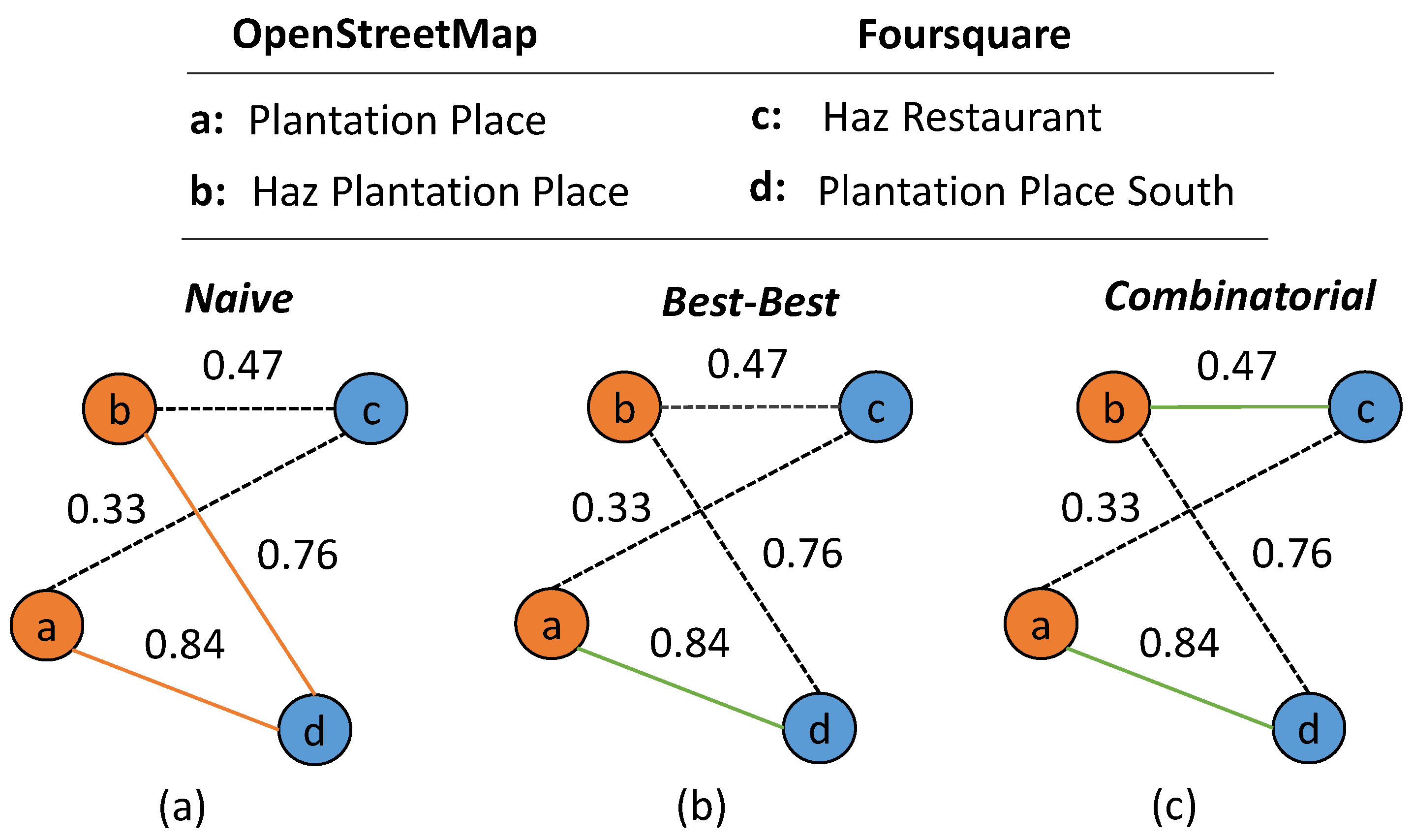
The third strategy we explored, named Combinatorial matching, performs matching in the graph-theory sense of the word. A matching solution is defined as a subset of the graph’s edges without common vertices. In our context, this means a matching solution without ambiguous matches. A graph may have many valid matching solutions. However, the Combinatorial matching strategy extracts the subset of edges with the highest sum of edge weights. This algorithm, developed by [49], when applied to bipartite graphs is also known as the weighted Hungarian combinatorial optimization algorithm [50]. The combinatorial matching solution for the graph in Figure 1a is depicted in Figure 1d. Despite ruling out ambiguous matches, this method has two drawbacks, namely, the best matching solution may discard strong edges (i.e., with large weights) depending on the graph’s structure and edge weights and it is not proper for detecting one-to-none matches. Despite that, in certain situations this method may perform better than the other two, as the example in Figure 2 demonstrates. The figure depicts a graph with nodes representing real POIs from OSM and Foursquare. The lower part of Figure 2 shows which nodes would be matched by the three strategies we explored if the edge weights were computed by the name similarity measure presented above. The Naïve strategy would produce an ambiguous match, whereas the Best-best strategy would match one of the POIs correctly while leaving the other incorrectly unmatched. The combinatorial approach, on the other hand, correctly matches both POIs by looking at the best subset of edges.
In order to overcome the drawback of the Combinatorial method that it may discard strong edges from the best subset of edges, the following transformation of the edge weights was undertaken. Firstly, the mean value of the edges connected to each node was computed. Because each edge connects two nodes, each edge has at this point two new values associated to it, namely, the mean values of the edges connected to each of its two nodes. Next, these two mean values were subtracted from the original weight of each edge. Lastly, the resulting numbers were summed. Figure 3 demonstrates these three steps based on a hypothetical graph whose combinatorial matching solution would not include the strongest edge of the graph. The effect of this edge weight transformation is that it increases the relative weight of originally strong edges while turning the weight of originally weak edges negative. This increases the chance that strong edges will belong to the best subset of edges and it will also exclude relatively weak edges from the subset, thus making this method able to perform one-to-none matchings as well. Another positive effect of this transformation of the edge weights is that it strongly mitigates performance issues. The Hungarian algorithm’s original time complexity is of O(number of nodes3), what practically made our experiments impossible to be performed on a regular computer. However, after the edge weight transformation, which, as demonstrated in Figure 3, transforms some of the edge weights to negative values and thus enables the elimination of such edges from the graph, the time taken for each experiment was in the order of 1 to 2 h.
2.4. Considering Multiple Entries from the Same Venue
As mentioned, frequently the same venue is represented by more than one POI in one or both of the datasets. Multiple entries from the same venue occur in VGI datasets when a user inattentively creates an already existing POI. When the same venue is represented as a building polygon and as a POI in the same VGI platform, a duplicated also entry occurs. We propose a simple yet effective rule-based strategy for finding hypothesis of redundant entries and considering them in the final matching result. The strategy consists of simple ’if, then’ queries that make a decision whether or not to include edges in the subset selected by the Best-best method. As an example, consider the two POI datasets distinguished by their colours in the figures above. The procedure starts by applying the Naïve matching method twice, namely once considering the blue dataset as the reference one and once considering the orange dataset as the reference one. Regarding the ambiguous edges from the first matching, the queries and decision depicted on Figure 4a are made. Likewise, the queries and decision depicted on Figure 4b are made regarding the outcome of the second naïve matching.
2.5. Experiment Design
For testing the matching strategies we proposed, a bounding-box of approximately 20 km2 located in the central area of London (England) was defined as test-area. The bounding box is circumscribed by the latitudes of 51 N and 51 N and the longitudes of 0 E and 01012 E. This area is one of the most vibrant from London and contains a large variety of commercial and leisure-related venues, like pubs, restaurants, cafés, shops, movies and museums. From this area, POI from the VGI platform OSM and the place review location-based social media Foursquare were collected. These two datasets have complementary strengths, as OSM is to most standards reliable regarding the position of POIs, whereas Foursquare contains mostly detailed semantic information about them. POI from OSM were extracted as node features with a name and at least one of the following tag keys: ‘amenity’, ’shop’, ’cuisine’, ’tourism’, ’office’, ’land-use’, ’leisure’, ’food’, ’sport’, ’use’, ’memorial’, ’type’ and ’brewery’. As not all POI are represented as points, OSM polygons (i.e. way features) with a name as well as with one of these tags and the ‘building:yes’ key/value pair were also collected. These OSM ways were transformed into points by associating its semantic data and position to the ways centres-of-mass. POIs from Foursquare were collected when their most detailed use category (see https://developer.foursquare.com/categorytree) was included in the set of categories from our test-samples. In total, 8238 POIs from OSM and 13,548 from Foursquare were collected.
For evaluating the performance of the different matching strategies, three types of test-samples were collected, as elucidated by Table 1. The one-to-one test-samples were built by randomly collecting 200 from the 8238 OSM POIs and finding their corresponding POIs in Foursquare. Five of these POIs had no corresponding ones in Foursquare and were thus considered as one-to-none test-samples. The remaining one-to-none as well as all one-to-many test-samples were collected by an exhaustive search in the OSM and Foursquare datasets from our test-area. Based on the parameters used in the t statistical test (explained below) for comparing the performance of the different matching strategies, calculations of the minimum sample size assuming a power of the test of 0.95 were performed. It is found that all three samples sizes are sufficiently large for all performance comparisons we conducted (see Section 3).
From the 21,786 POIs collected from OSM and Foursquare, a graph was created by setting an edge between nodes belonging to different datasets and located closer than 100 m from each other. The resulting graph, with a total of 339,974 edges, was used in the application of the graph-based matching strategies we propose in this paper. The distance threshold of 100 m was defined after analyzing the histogram of the distances between the 229 pairs of one-to-one and one-to-many matches from our test-samples set (Table 1). This histogram is depicted in Figure 5. The construction of the graph took about 15 min in a conventional computer, which indicates that scaling our graph-based matching strategies to larger test-areas is not expected to cause computational issues.
In order to evaluate the statistical difference in the performance of the different matching strategies, the following t statistic was computed as suggested by [51] for the comparison of accuracy percentages:
where and are the percentages of correctly matched pairs from two different matching experiments (computed based on the test-samples), p is the average between and , q is the difference between 1 and p and n is the number of test-samples. The two compared matching accuracies will be different if , where is the test’s significance level. The critical value of is computed from a t distribution of degrees of freedom. In the next section, we compare the p-values from different pairs of matching accuracies with = 0.025 and 0.05.
3. Results
The performances of the POI matching strategies were evaluated in three different analyses. In the first, we considered 229 matching pairs from which 195 are perfect one-to-one matches and 34 are matches containing at least one of its POI in another one of these 34 pairs. These 34 pairs were included in order to evaluate our strategy for detecting one-to-many matches, i.e. cases in which a POI should be matched with more than one POI from the other dataset. In the second analysis, we evaluated based on 42 POIs from OSM the strategies performance in correctly leaving POIs from OSM unmatched when these have no corresponding ones in Foursquare. The third analysis considered all test-samples together. Each of these three analyses was carried out with different combinations of similarity measures aggregated by their unweighted and weighted sum.
Figure 6a,b show the percentage of the 229 one-to-one test-sample pairs correctly matched by each of the three matching strategies applied with different combinations of similarity measures aggregated by their unweighted (Figure 6a) and weighted sums (Figure 6b). It can be seen that the accuracy achieved by the Naïve method is the highest in all cases, followed mostly by the Combinatorial method. Regarding Figure 6a and the Naive method, the matching accuracies achieved with different combinations of similarity measures are not statistically different (i.e., p-values well above 0.05) from the accuracy of the matching performed only with the string similarity (of 93%). The matching accuracies achieved with the Combinatorial method based on different combinations of similarity measures are also not statistically different from the accuracy achieved with the string similarity alone. In the case of the Best-Best method, the matching accuracy decreased significantly (p-value < 0.025) when the semantic and spatial similarities were also considered, as opposed to when the matching was performed only based on the string similarity. Comparing Figure 6a,b, it is noticeable that all three methods achieved higher accuracy levels when the similarity measures were aggregated by their weighted sum. This holds for all three measure combinations. However, the increase in the accuracy is in all nine cases not statistically significant. It should be stressed though that the Naive method applied based on the spatial and string similarities has experienced an increase of 5% in the performance (from 89% to 94%) when these measures were aggregated by their weighted sum. The statistical comparison of this difference in the performance yielded a p-value of 0.056. The Combinatorial method applied with the string and semantic similarities also experienced an increase of 5% in the accuracy (from 77% to 82%). However, the large p-value of 0.18 for the significance of this increase does not allow the claiming of a statistical improvement.
Figure 6c,d depict the one-to-none accuracies evaluated based on 42 POIs from OSM with no corresponding POI in Foursquare. The better performance of the Best-best method is statistically significant when considering the string and semantic similarities aggregated by their unweighted sum (p-value of 0.038) as well as in all three cases when the similarity measures are aggregated by their weighted sum (Figure 6d) (p-values < 0.021). It is also noticeable that the weighted sum of the similarity measures has led to a decrease in this type of accuracy, which is however in none of the cases significant.
Figure 6e,f depict the accuracy levels obtained with the one-to-one and one-to-many samples (229) together with the one-to-none samples (42). It can be observed that the Naïve method is mostly the one that performed the worst, as it is incapable of detecting one-to-none matches. The Best-best method in the other hand is the one that achieved the highest accuracy levels in all comparisons from Figure 6e,f. This superior performance is however statistically significant only regarding the matchings conducted with the string similarity (p-value of 0.032). It is also worth noticing that, although statistically not significant, the weighted sum aggregation of the similarity measures led to better accuracies than the unweighted sum aggregation. The overall best accuracy however was achieved by the Best-best method based only on the POIs string similarity (86%).
In summary, from Figure 6 the following conclusions can be made. Concerning the one-to-one matchings, the Naive method performed best. For detecting one-to-none cases, the Best-best method is by far superior to the Combinatorial method. When all three different types of test-samples are considered, the Best-best method emerged as the most effective, followed in general by the Combinatorial method. Aggregating the similarity measures by their weighted sum led in general to slight increases in the performance, which are however not statistically significant. It can be claimed that the overall best matching accuracies were achieved with the Best-best method based on the string similarity alone (accuracy of 86%, as mentioned) and based on the string and spatial similarities aggregated by their weighted sum (accuracy of 84%).
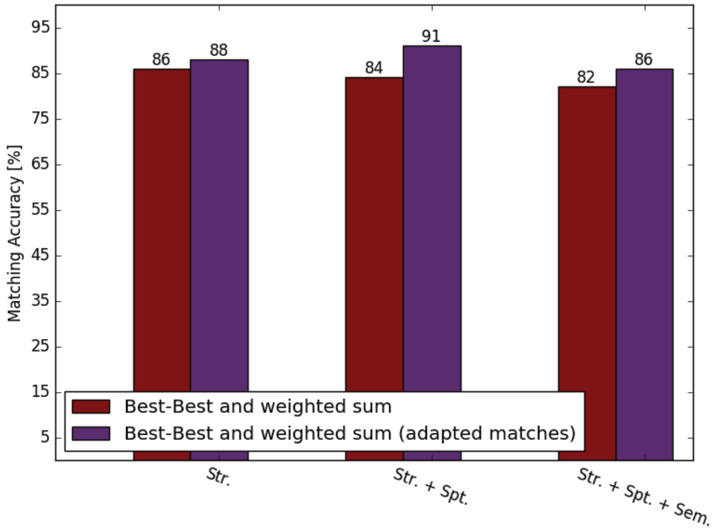
In Section 2.4, we presented a simple procedure for dealing with cases when a place is represented by more than one POI in one or both of the datasets. Figure 7 depicts the increase in the accuracy levels achieved when applying this procedure over the matches obtained with the Best-best method considering three different combinations of similarity measures aggregated by their weighted sum. These combinations were selected due to their better performances (see Figure 6e,f). It can be seen that for the three different similarity combinations, an improvement of accuracy was achieved. This improvement is of 7% (i.e., from 84% to 91%) and statistically significant (p-value of 0.014) when the string and spatial similarities are considered, thus giving evidence that the proposed procedure is effective. This also indicates that considering the spatial and string similarities, as opposed to just the string similarity, is advantageous, although the accuracy difference between these two matching strategies (of 91% and 88%, respectively) is not statistically significant.
4. Summary and Discussion
In this paper, we focused on the matching aspect of the conflation of POI from VGI platforms. The strategies we proposed are based on a graph whose nodes represent the POI from two different platforms and the edges their matching possibilities. We showed how the graph can be used for dynamically defining the weights of the similarity measures which are then summed up to a final edge weight based on which the matching is performed. The results attest that the weighted sum of the similarity measures leads in general to better, although mostly not statistically significant, matching accuracies in comparison to when the similarities are summed with equal weights. Furthermore, we demonstrated how the graph enabled us to perform one-to-none as well as one-to-many and many-to-one matches. These types of matches must absolutely be considered if the semantic information from POI from different collaborative sources is to be properly conflated. Surprisingly though, to the best of our knowledge, methods for accounting in the matching for the very current situations of duplicated and absent POI in datasets with different purposes but complementary geographic information were still lacking.
It is important to point out that neither the edges final weight computation nor the matching strategies we proposed require time-costly collection of training samples. Because of that, our methods can be more easily integrated into broader workflows with goals beyond the POI conflation step. Furthermore, unsupervised POI matching methods tend to be more transferable than supervised methods, which, although possibly more effective in a specific area, involve the risk of over-fitting and therefore of poor transferability.
The perspective seems reasonable that many geographic studies and geospatial applications will continue to rely more and more on up-to-date and semantically detailed user-generated information from urban features. As this information will unlikely be stored in a single platform, but rather in a growing number of collaborative geo-data platforms with different purposes and limitations (but of complementatry strengths), POI conflation methods able to deal with the inherent characteristics of user-generated geo-data will increasingly be required. It is therefore imperative that the different technical challenges for achieving this increasingly complex interoperability of geo-datasets be one of the main objects of current research in geoinformatics. This paper is inserted in this very context as it proposes POI matching methods that account for two typical characteristics of collaborative POI datasets, namely, incompleteness and redundancy. Our main motivation was to contribute effective and transferable POI matching methods that are more general than purpose, case and-data- specific solutions.
From our perspective, future research possibilities in this area include the development of higher-order matching methods, i.e., the simultaneous matching of POIs from more than two datasets, as a way of possibly achieving better performance than pairwise matching methods. The principles from our two graph-based matching strategies (i.e., collective and combinatorial matching and mutual agreement) can maybe be explored for higher-order POIs matching as well. Although we made the argument that one of the main advantages of the matching strategies we propose is that they do not require training, it would be pertinent to explore supervised methods for computing the edges weights. The final edges weights might, by the way, be a function of other similarity measures like topic, topological, geocoding (i.e., address) and temporal activity similarities as well. Obviously, this will depend on the geo-datasets being conflated and on the degree of completeness they have for these different types of information. The exploration of more comprehensive POIs similarity measures might also benefit strategies for matching VGI POIs with social media posts related (to different degrees of relevance) to a specific place. These methods need to be continuously adapted as novelties appear on social media types and activities as well as on the possibilities of relating (explicitly and implicitly) a post to a place.
Acknowledgments
We acknowledge financial support by Deutsche Forschungsgemeinschaft (DFG) within the funding programme Open Access Publishing, by the Baden-Württemberg Ministry of Science, Research and the Arts and by Ruprecht-Karls-Universität Heidelberg. This and other related research is being supported by DFG, project number 276698709.
Author Contributions
All three authors contributed extensively to the work presented in this paper.
Conflicts of Interest
The authors declare no conflict of interest.
References
- Jonietz, D.; Zipf, A. Defining fitness-for-use for crowdsourced points of interest (POI). ISPRS Int. J. Geo-Inf. 2016, 5, 149. [Google Scholar] [CrossRef]
- Touya, G.; Antoniou, V.; Olteanu-Raimond, A.-M.; Van Damme, M.-D. Assessing crowdsourced POI quality: Combining methods based on reference data, history, and spatial relations. ISPRS Int. J. Geo-Inf. 2017, 6, 80. [Google Scholar] [CrossRef]
- Ballatore, A.; Zipf, A. A conceptual quality framework for volunteered geographic information. In Proceedings of the XII Conference on Spatial Information Theory, Santa Fe, NM, USA, 12–16 October 2015. [Google Scholar]
- Senaratne, H.; Mobasheri, A.; Ali, A.L.; Capieri, C.; Haklay, M. A review of volunteered geographic information quality assessment methods. Int. J. Geogr. Inf. Sci. 2016, 31, 139–167. [Google Scholar] [CrossRef]
- Degrossi, L.C.; Albuquerque, J.P.D.; Rocha, R.D.S.; Zipf, A. A framework of quality assessment methods for crowdsourced geographic information: A systematic literature review. In Proceedings of the 14th International Conference on Information Systems for Crisis Response and Management, Albi, France, 21–24 May 2017. [Google Scholar]
- Li, L.; Goodchild, M.F. An optimisation model for linear feature matching in geographical data conflation. Int. J. Image Data Fusion 2011, 2, 309–328. [Google Scholar] [CrossRef]
- Abdolmajidi, E.; Mansourian, A.; Will, J.; Harrie, L. Matching authority and VGI road networks using an extended node-based matching algorithm. Geo-Spat. Inf. Sci. 2015, 18, 65–80. [Google Scholar] [CrossRef]
- Hetch, R.; Kunze, C.; Hahmann, S. Measuring completness of building footprints in OpenStreetMap over space and time. ISPRS Int. J. Geo-Inf. 2013, 2, 1066–1091. [Google Scholar]
- Fan, H.; Zipf, A.; Fu, Q.; Neis, P. Quality assessment for building footprints data on OpenStreetMap. Int. J. Geogr. Inf. Sci. 2014, 28, 700–719. [Google Scholar] [CrossRef]
- Rutta, M.; Scioscia, F.; De Filippis, D.; Ieva, S.; Binetti, M.; Di Sciasco, E. A semantic-enhanced augmented reality tool for OpenStreetMap POI discovery. Transp. Res. Procedia 2014, 3, 479–488. [Google Scholar] [CrossRef]
- Guo, L.; Jiang, H.; Wang, X.; Liu, F. Learning to recommend point-of-interest with the weighted bayseian personalized ranking method in LBSNs. Information 2017, 8, 20. [Google Scholar] [CrossRef]
- Bakillah, M.; Liang, S.; Mobasheri, A.; Arsanjani, J.J.; Zipf, A. Fine-resolution population mapping using OpenStreetMap points-of-interest. Int. J. Geogr. Inf. Sci. 2014, 48, 1940–1963. [Google Scholar] [CrossRef]
- Jiang, S.; Alves, A.; Rodrigues, F.; Ferreira, J.; Pereira, F.C. Mining point-of-interest data from social networks for urban land use classification and disaggregation. Comput. Environ. Urban Syst. 2015, 53, 36–46. [Google Scholar] [CrossRef]
- Kunze, C.; Hecht, R. Semantic enrichment of building data with volunteered geographic information to improve mappings of dwelling units and population. Comput. Environ. Urban Syst. 2015, 53, 4–18. [Google Scholar] [CrossRef]
- Niu, N.; Liu, X.; Jin, H.; Ye, X.; Liu, Y.; Li, X.; Chen, Y.; Li, S. Integrating multi-source big data to infer building functions. Int. J. Geogr. Inf. Sci. 2017, 31, 1871–1890. [Google Scholar] [CrossRef]
- Calegari, G.R.; Carlino, E.; Peroni, D.; Celino, I. Extracting urban land use from linked open geospatial data. ISPRS Int. J. Geo-Inf. 2015, 4, 2109–2130. [Google Scholar] [CrossRef]
- Arsanjani, J.J.; Helbich, M.; Bakillah, M.; Hagenauer, J.; Zipf, A. Toward mapping land-use patterns from volunteered geographic information. Int. J. Geogr. Inf. Sci. 2013, 27, 2264–2278. [Google Scholar] [CrossRef]
- Liu, X.; Long, Y. Automated identification and characterization of parcels with OpenStreetMap and points of interest. Environ. Plan. B Plan. Des. 2016, 42, 341–360. [Google Scholar] [CrossRef]
- Yang, B.; Zhang, Y.; Lu, F. Geometric-based approach for integrating VGI POIs and road networks. Int. J. Geogr. Inf. Sci. 2014, 28, 126–147. [Google Scholar] [CrossRef]
- Yang, B.; Zhang, Y. Pattern-mining approach for conflating crowdsourcing road networks with POIs. Int. J. Geogr. Inf. Sci. 2015, 29, 786–805. [Google Scholar] [CrossRef]
- Pouke, M.; Goncalves, J.; Ferreira, D.; Kostakos, V. Pratical simulation of virtual crowds using points of interests. Comput. Environ. Urban Syst. 2015, 57, 118–129. [Google Scholar] [CrossRef]
- Sun, Y. Investigating “locality” of intra-urban spatial interactions in New York city using Foursquare data. Int. J. Geo-Inf. 2016, 5, 43. [Google Scholar] [CrossRef]
- Fang, Z.; Li, Q.; Zhang, X.; Shaw, S.-L. A GIS data model for landmark-based pedestrian navigation. Int. J. Geogr. Inf. Sci. 2012, 26, 817–838. [Google Scholar] [CrossRef]
- Roussel, A.; Zipf, A. Toward a landmark-based pedestrian navigation service using OSM data. Int. J. Geo-Inf. 2017, 6, 64. [Google Scholar] [CrossRef]
- Delgado, F.; Martínez-Gonzales, M.M.; Finat, J. An evaluation of ontology matching techniques on geospatial ontologies. Int. J. Geogr. Inf. Sci. 2013, 27, 2279–2301. [Google Scholar] [CrossRef]
- Mckenzie, G.; Janowicz, K.; Adams, B. Weighted multi-attribute matching of user-generated points of interest. Cartogr. Geogr. Inf. Sci. 2014, 41, 125–137. [Google Scholar] [CrossRef]
- Li, L.; Xing, X.; Xia, H.; Huang, X. Entropy-weighted instance matching between different sourcing points of interest. Entropy 2016, 18, 45. [Google Scholar] [CrossRef]
- Novack, T.; Peters, R.; Zipf, A. Graph-based strategies for matching points-of-interests from different VGI sources. In Proceedings of the 20th AGILE Conference, Wageningen, The Netherlands, 9–12 May 2017. [Google Scholar]
- Vasardani, M.; Winter, S.; Richter, K.F. Locating place names from place descriptions. Int. J. Geogr. Inf. Sci. 2013, 27, 2509–2532. [Google Scholar] [CrossRef]
- Kim, J.; Vasardani, M.; Winter, S. Similarity matching for integrating spatial information extracted from place descriptions. Int. J. Geogr. Inf. Sci. 2017, 31, 56–80. [Google Scholar] [CrossRef]
- Scheffer, T.; Schirru, R.; Lehmann, P. Matching points of interest from different social networking sites. In KL 2012: Advances in Artificial Intelligence; Glimm, B., Krüger, A., Eds.; Springer: Berlin, Germany, 2012; pp. 245–248. ISBN 978-3-642-33346-0. [Google Scholar]
- Cohen, W.W.; Ravikumar, P.; Fienberg, S.E. A comparison of string distance metrics for name-matching tasks. In Proceedings of the 2003 International Joint Conferences on Artificial Intelligence (IJCAI-03), Acapulco, Mexico, 9–10 August 2003. [Google Scholar]
- Meltzoff, A.N.; Kuhl, P.K.; Movellan, J.; Sejnowski, T.J. Foundations for a new science of learning. Science 2009, 325, 284–288. [Google Scholar] [CrossRef] [PubMed]
- Liu, W.; Cai, M.; Yuan, H.; Shi, X.; Zhang, W.; Liu, J. Phonotactic language recognition based on Dnn-HMM acoustic model. In Proceedings of the 9th International Symposium on Chinese Spoken Language Processing (ISCSLP), Singapore, 12–14 September 2014; pp. 153–157. [Google Scholar]
- Ballatore, A.; Bertolotto, M.; Wilson, D.C. The semantic similarity ensemble. J. Spat. Inf. Sci. 2016, 7, 27–44. [Google Scholar] [CrossRef]
- Blei, D.M.; Ng, A.Y.; Jordan, M.I. Latent Dirichlet Allocation. J. Mach. Learn. Res. 2003, 3, 993–1022. [Google Scholar]
- Rodrigues, F.; Alves, A.; Polisciuc, E.; Jiang, S.; Ferreira, J.; Pereira, F.C. Estimating disaggregated employment size from points-of-interest and census data: From mining the web to model implementation and visualization. Int. J. Adv. Intell. Syst. 2013, 6, 41–52. [Google Scholar]
- Olteanu-Raimond, A.M.; Mustière, S.; Ruas, A. Knowledge formalization for vector data matching using belief theory. J. Spat. Inf. Sci. 2015, 10, 21–46. [Google Scholar] [CrossRef]
- Foursquare. Available online: https://foursquare.com/about (accessed on 11 January 2018).
- Yelp. Available online: https://www.yelp.com/about (accessed on 11 January 2018).
- Levenshtein, V.I. Binary codes capable of correcting deletions, insertions and reversals. Sov. Phys. Dokl. 1966, 10, 707–710. [Google Scholar]
- Bonzanini, M. Fuzzy String Matching in Python. Available online: https://marcobonzanini.com/2015/02/25/fuzzy-string-matching-in-python/ (accessed on 12 March 2018).
- Miller, G.A. WorldNet: A lexical database for English. Commun. ACM 1995, 38, 39–41. [Google Scholar] [CrossRef]
- Meng, L.; Huang, R.; Gu, J. A review of semantic similarity measures in WordNet. Int. J. Hybrid Inf. Technol. 2013, 6, 1–12. [Google Scholar]
- Sánchez, D.; Batet, M. A semantic similarity method based on information content exploiting multiple ontologies. Expert Syst. Appl. 2013, 40, 1393–1399. [Google Scholar] [CrossRef]
- Al-Bakri, M.; Fairbairn, D. Assessing similarity matching for possible integration of feature classifications of geospatial data from official and informal sources. Int. J. Geogr. Inf. Sci. 1995, 26, 1437–1456. [Google Scholar] [CrossRef]
- Lin, D. An information-theoretic definition of similarity. In Proceedings of the 15th International Conference on Machine Learning, Madison, WI, USA, 24–27 July 1998. [Google Scholar]
- Landes, S.; Leacock, C.; Fellbaum, C. Building semantic concordances. In WordNet: An Electronical Lexical Database; Fellbaum, C., Ed.; The MIT Press: London, UK, 1998; pp. 199–216. [Google Scholar]
- Galil, Z. Efficient algorithms for finding maximal matching in graphs. J. ACM Comput. Surv. 1986, 18, 23–38. [Google Scholar] [CrossRef]
- Kuhn, H.W. The Hungarian method for assignment problems. Nav. Res. Logist. Q. 1955, 3, 253–258. [Google Scholar] [CrossRef]
- Zwillinger, D.; Kokosa, S. Standard Probability and Statistics Tables and Formulae; Chapman and Hall: London, UK, 2000; p. 480. [Google Scholar]
Figure 1.
(a) A hypothetical graph. Nodes represent POI and edges matching pair candidates; (b) Matching result obtained with the Naïve method; (c) Matching result obtained with the Best-best method; (d) Matching result obtained with the Combinatorial method.
Figure 1.
(a) A hypothetical graph. Nodes represent POI and edges matching pair candidates; (b) Matching result obtained with the Naïve method; (c) Matching result obtained with the Best-best method; (d) Matching result obtained with the Combinatorial method.
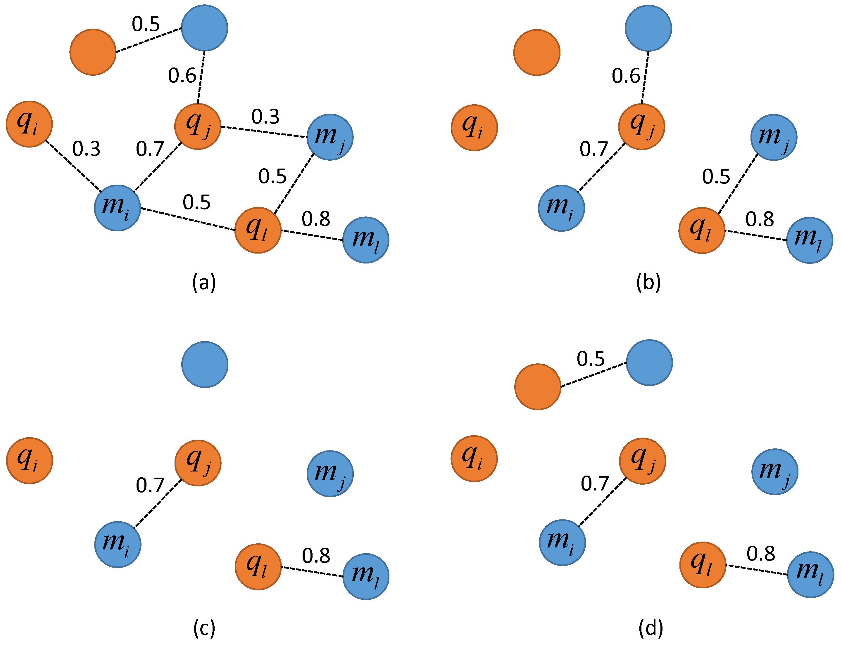
Figure 2.
Graph representing four existing POIs from OSM and Foursquare. (a–c) Matching results obtained with the three different strategies investigated in this work. Edge weights were computed with the name similarity measure presented in Section 2.1.
Figure 2.
Graph representing four existing POIs from OSM and Foursquare. (a–c) Matching results obtained with the three different strategies investigated in this work. Edge weights were computed with the name similarity measure presented in Section 2.1.

Figure 3.
Transformation applied to the graph’s edges weights before applying the Combinatorial matching strategy. (a) The graph and its original edge weights; (b) Mean values of the edges connected to each node; (c) Original edge weights minus the mean values computed in the previous step; (d) New edge weights resulting from the summation of the values obtained in the previous step.
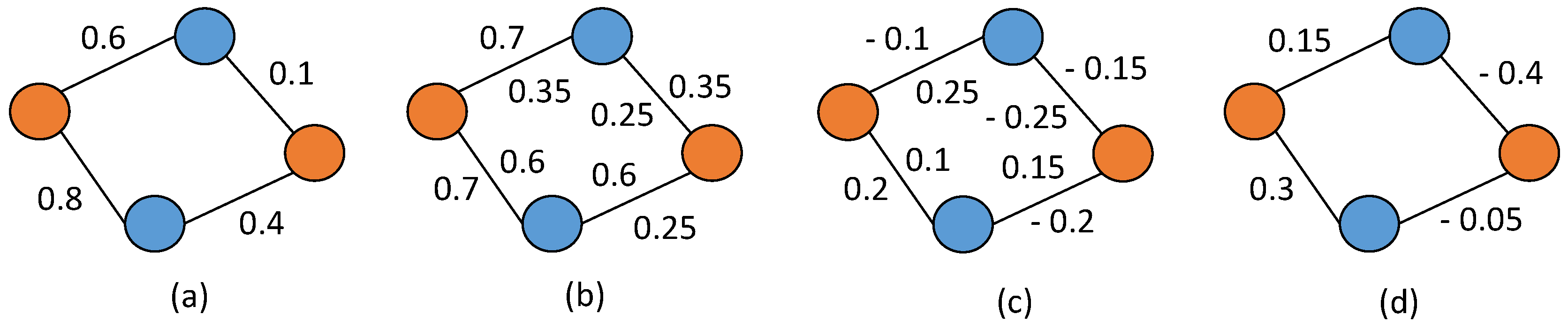
Figure 4.
Queries applied for including edges in the subset of edges extracted by the Best-best method. (a) Queries and decision applied to the ambiguous edges obtained by applying the Naïve method taking the blue dataset as the reference one; (b) Queries and decision applied to the ambiguous edges obtained by applying the Naïve method taking the orange dataset as the reference one.
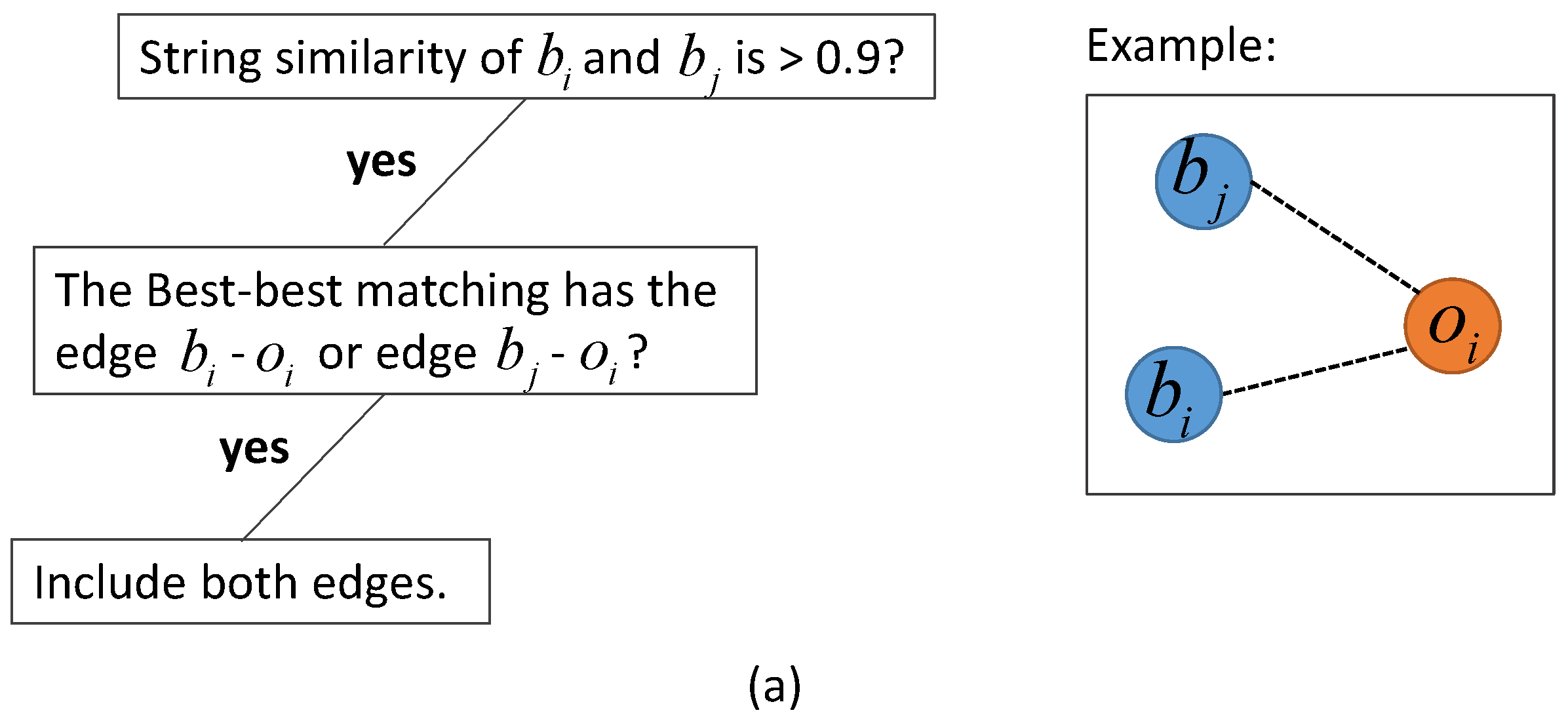
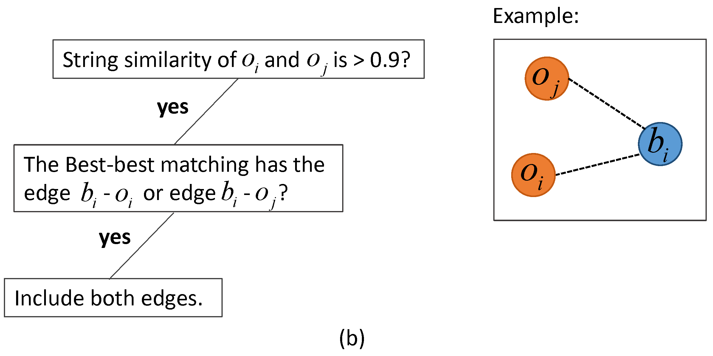
Figure 5.
Histogram of the distances between the pairs of matching POI from OSM and Foursquare comprising our test-sample set.
Figure 5.
Histogram of the distances between the pairs of matching POI from OSM and Foursquare comprising our test-sample set.
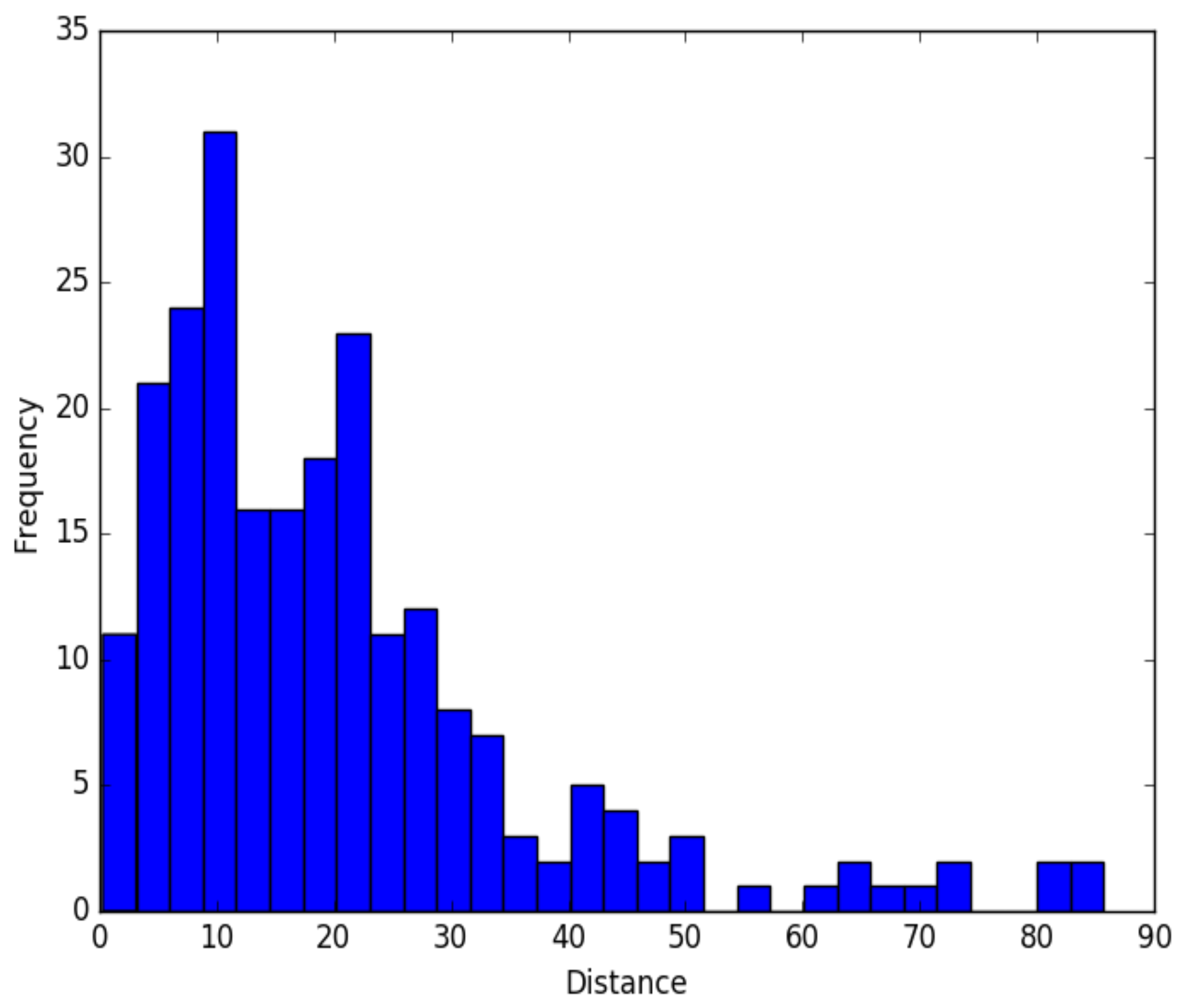
Figure 6.
Evaluation of the different matching strategies applied with different similarity measures aggregated by their unweighted and weighted sum. (a,b) One-to-one and one-to-many matching accuracies obtained with the three different strategies and similarity measures aggregated by their unweighted (a) and weighted sum (b). (c,d) One-to-none matching accuracies obtained with the Best-best and Combinatorial strategies and similarity measures aggregated by their unweighted (c) and weighted sum (d). (e,f) Overall accuracies with similarity measures aggregated by their unweighted (e) and weighted sums (f).
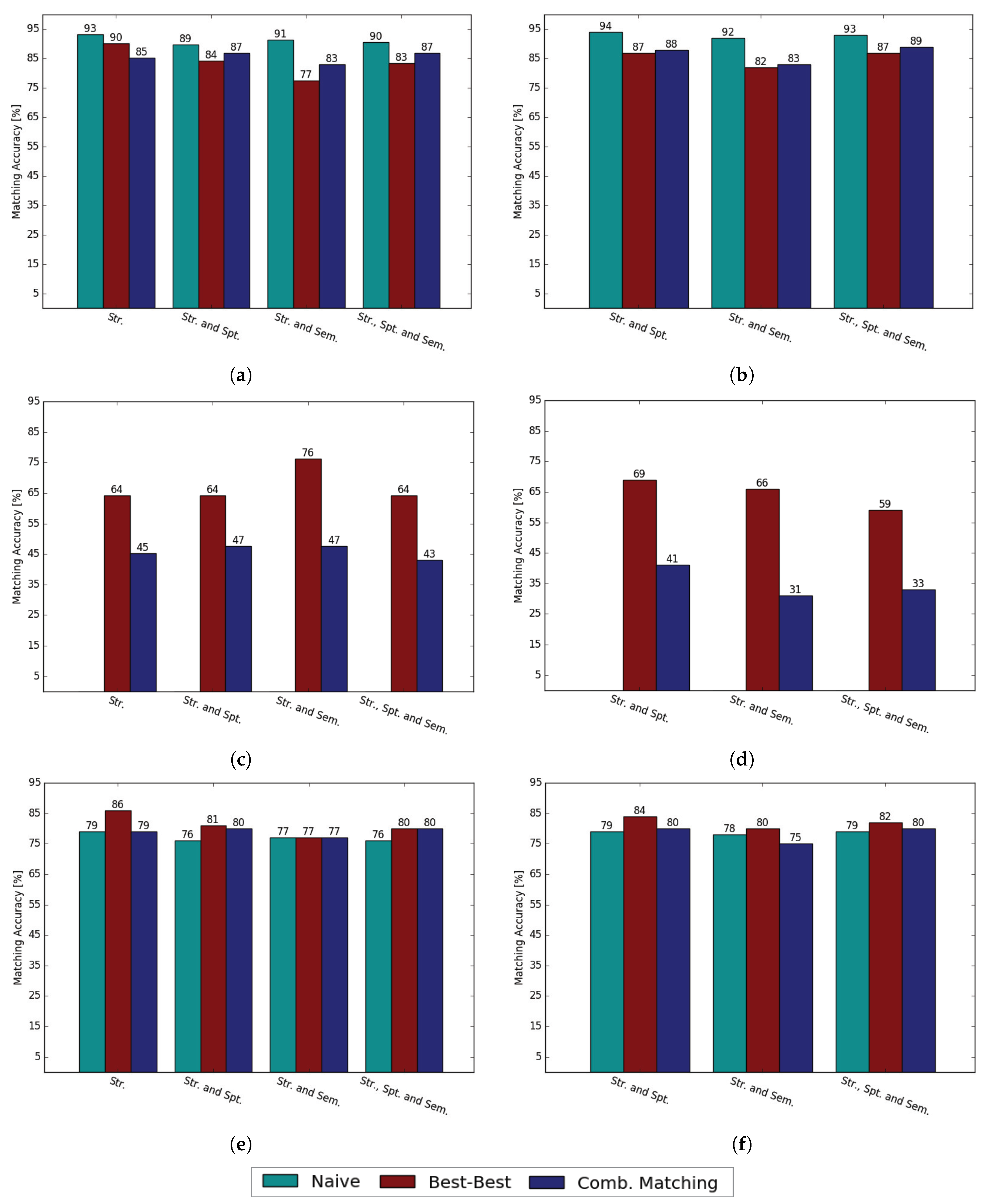
Figure 7.
Matching accuracies obtained before and after applying the procedure for tackling the existence of multiple POIs representing the same place.
Figure 7.
Matching accuracies obtained before and after applying the procedure for tackling the existence of multiple POIs representing the same place.


Table 1.
The different types and respective amounts of test-samples considered in the performance analysis of the different matching strategies.
Table 1.
The different types and respective amounts of test-samples considered in the performance analysis of the different matching strategies.
| Sample Types | Purpose Is to Evaluate the Models Performance in Detecting … | Amount |
|---|---|---|
| One-to-one | Cases when a POI from OSM should be matched with only one POI from Foursquare and vice-versa. | 195 |
| One-to-none | Cases when a POI from OSM does not have any match in Foursquare and should therefore be left unmatched. | 42 |
| One-to-many | Cases when more than one POI from OSM should be matched to the same Foursquare POI and cases when more than one POI from Foursquare should be matched to the same POI from OSM. | 34 |
© 2018 by the authors. Licensee MDPI, Basel, Switzerland. This article is an open access article distributed under the terms and conditions of the Creative Commons Attribution (CC BY) license (http://creativecommons.org/licenses/by/4.0/).
Share and Cite
MDPI and ACS Style
Novack, T.; Peters, R.; Zipf, A. Graph-Based Matching of Points-of-Interest from Collaborative Geo-Datasets. ISPRS Int. J. Geo-Inf. 2018, 7, 117. https://doi.org/10.3390/ijgi7030117
AMA Style
Novack T, Peters R, Zipf A. Graph-Based Matching of Points-of-Interest from Collaborative Geo-Datasets. ISPRS International Journal of Geo-Information. 2018; 7(3):117. https://doi.org/10.3390/ijgi7030117
Chicago/Turabian StyleNovack, Tessio, Robin Peters, and Alexander Zipf. 2018. "Graph-Based Matching of Points-of-Interest from Collaborative Geo-Datasets" ISPRS International Journal of Geo-Information 7, no. 3: 117. https://doi.org/10.3390/ijgi7030117
Note that from the first issue of 2016, this journal uses article numbers instead of page numbers. See further details here.