Article

Study on Multi-Scale Window Determination for GLCM Texture Description in High-Resolution Remote Sensing Image Geo-Analysis Supported by GIS and Domain Knowledge

1
School of management, Guangdong University of Technology, 169 Yinglong Road, Guangzhou 510520, China
2
Geographic Information Department, Guangzhou Urban Planning & Design Survey Research Institute, 10 Jianshe Road, Guangzhou 510060, China
*
Author to whom correspondence should be addressed.
ISPRS Int. J. Geo-Inf. 2018, 7(5), 175; https://doi.org/10.3390/ijgi7050175
Submission received: 18 March 2018 / Revised: 26 April 2018 / Accepted: 28 April 2018 / Published: 5 May 2018
(This article belongs to the Special Issue Leading Progress in Digital Terrain Analysis and Modeling)

Abstract

:
Texture features based on the gray-level co-occurrence matrix (GLCM) can effectively improve classification accuracy in geographical analyses of optical remote sensing (RS) images, with the parameters of scale of the GLCM texture window greatly affecting the validity. By analyzing human visual attention characteristics for geo-texture cognition, it was found that there is a strong correlation between the texture scale parameters and the domain shape knowledge in a specified geo-scene. Therefore, a new approach for quickly determining the multi-scale parameters of the texture with the assistance of a geographic information system (GIS) and domain knowledge is proposed in this paper. First, the validity of domain knowledge from an existing GIS database is measured by spatial data mining algorithms, including spatial partitioning, image segmentation, and space-time system evaluation. Second, the general domain shape knowledge of each category is described by the GIS minimum enclosing rectangle indices and rectangular-degree indices. Then, the corresponding multi-scale texture windows can be quickly determined for each category by a correlation analysis with the shape indices. Finally, the Fisher function is used to evaluate the validity of the scale parameters. The experimental results show that the multi-scale value keeps a one-to-one relationship with the classified objects, and their value ranges are from a few to tens, instead of the smaller values of a traditional analysis; thus, effective texture features at such a scale can be built to identify categories in a geo-scene. In this way, the proposed method can increase the total number of categories for a certain geo-scene and reduce the classification uncertainty, as well as better meet the requirements of large-scale image geo-analysis. It also has as high a calculation efficiency and as good a performance as the traditional enumeration method.

1. Introduction

Texture is an important image spatial feature [1,2,3]. Many texture descriptors have been developed in the past, such as frequency domain analysis based on the Fourier transform, the wavelet transform approach, the hidden Markov approach, the local binary pattern (LBP), the local multiple patterns (LMP), the geostatistical-based approach, the watershed-based approach, the gray-level co-occurrence matrix (GLCM)-based approach, and other statistical approaches [2,3,4,5,6,7,8,9,10,11,12,13,14,15,16,17,18]. Most of these approaches are mainly designed for a simple and clear classification system or a specific object, similar to in the fields of medicine, industry, the military, etc. [3,4,5,6,7,8,9,10,11,12,13,14,15,16,17,18]. However, when using high-resolution optical remote sensing (RS) images for geographical classification, the classification system will change with the needs of different geo-scenes, even in the same image, so the phenomena of “same object different spectrum”, “same spectrum different object”, and “mixed pixels” will become more prevalent, and the textures will be more complex and changeable [1,2,19,20,21,22,23,24,25,26,27,28,29,30]. Scholars have emphasized that such image analysis can be improved by employing geo-domain knowledge (especially various general statistical characteristics such as topology, location, spatial relationship, etc.) [19,20,21,22,23,24,25,26,27,28,29,30]. Thus, in this paper, a GLCM-based approach that can be easily associated with geo-knowledge is chosen to build texture features for geo applications. This is because the GLCM obtains statistics by using a certain scale window, where one can intuitively observe the actual objects and reflect the domain knowledge (mainly spatial shape attributes). Moreover, it provides information in image gray direction, interval and change amplitude, so that 14 kinds of texture features can be effectively defined based on it [3], and it meets the requirement for the classification of complex and variable geo-scenes [31].
Since 1990, scientists have created studies on the impact of various parameters on the validity of GLCM-based texture, and they found that it is very sensitive to the scale parameter, and the classification accuracy can even decrease if the parameter is unreasonable [31,32,33,34,35,36]. Marceau D.J. (1990) first used SOPT data to conduct a quantified study [31]. He used the factor analysis method to measure the impact on window size, quantization level, and four texture statistics (Energy, Contrast, Homogeneity, Entropy) for land cover types. The impacts are as follows: the scale of the window has the greatest effect on the classification, followed by the texture statistics, and the least significant is the level of quantization [31]. Later, other researchers also successively obtained similar study results [32,33,34,35,36,37]. In Cui L.’s Ph.D. dissertation (2005), this issue was described in depth [32]. She measured the impact on window scale, direction and level of quantization, and found that different directions had little effect on the classification reliability of most types, and the best solution was to use the average value of the omni direction. Different bands play a crucial role in the extraction of texture features for multispectral TM data, so the use of combined band information is important. In addition, she took the scale parameters from 3 to 50 separately for the TM image analysis and found the variation rule of 8 GLCM texture features of 14 types of geo-objects by using the enumerated window scale. She found that there was a correspondence between the different texture features and the different windows. When the window was small, the feature space composed of a combination of 2 texture features achieved good results. When the window was gradually increased, the combination dimension of the texture feature space was also increased, and the combination of 5 texture features achieved best results. Moreover, she found that the overall classification accuracy gradually increased with scale, reaching the highest value when the scale reached 35. Therefore, she concluded that the optimal identification windows of different objects were different, although only an optimal scale of 35 was used in the subsequent classification [32]. That is, multi-scale is an essential and necessary feature of spatial data, and it has a significant impact on GLCM-based texture features [31,32,33,34,35,36,37,38,39,40,41,42,43].
In many practical applications, the choice of scale parameters is still very arbitrary when using empirical method, and a small scale value is commonly chosen, either 3, 5, 7 or 9. It is easy to operate, but also extremely unreliable [32,33,34]. In addition, researchers have also developed various statistical methods for analyzing texture scales, including a histogram algorithm, a variogram algorithm, a Markov algorithm, a mean shift algorithm, and a fractal network evolutionary algorithm of Ecognition, etc. [1,8,9,10,11,12,13,14,15,16,17,18]. Additionally, Binaghi, E. et al. (2003) set the scale parameters by taking the statistics of the spatial characteristics of sampled data [43]. These methods can sometimes obtain multi-scale parameters. Therefore, they are able to achieve adaptive estimation to some extent and can improve the validity of texture features. However, the number of scales was random and few, and the values of the scales were usually low. In terms of the algorithms themselves, local optima or independent of actual categories will appear easily if they rely too much on the sample selection or the local image gray level variability analysis, or the errors will accumulate if they adopt an iterative calculation model. It can be seen that there are still many uncertainties in current studies for the selection of texture scale [31,32,33,34,35,36,37,38,39,40,41,42,43,44]. Some are only aimed at a certain application, some are only able to obtain a single scale parameter, and some are able to obtain multi-scales, but each time the results are commonly inconsistent and small for the number and value of scales. Therefore, it is necessary to find a quick and reliable setting method for multi-scale image texture in geo-analysis.
To solve the problems above, this paper proposes a new method for determining multi-scale windows of image GLCM texture descriptors by means of the integrated use of a geographic information system (GIS) and geo-spatial domain knowledge. First, we explain the rules for the changes in texture scales under different geo-scenes and classification systems and construct a framework for texture scale recognition and extraction by simulating human visual attention and interpretation characteristics [1,2,19,20,21,22,23,24,25,26,27,28,29]. Second, a body of effective geo-spatial domain knowledge is mined from an existing GIS database. Then, the link between domain knowledge and texture scale is established, so that multi-scale windows can be quickly determined for each category. The approach uses geo domain knowledge that is extracted from different GIS informative layers (which is likely to be cheap to source from historical databases) to define the characteristic size and shape of the geo-scene categories of interest. These informative layers can be topographic maps, digital elevation models (DEM), land-use maps, etc. It must be noted that there is a possibility that these maps could cover a wide temporal range, and due to this potential temporal variability of the landscape, the accuracy of the domain knowledge should be taken into account. Finally, the Fisher function analysis based on the enumeration method is used to evaluate the validity of the above multi-scale parameters [44,45,46,47]. In this paper, experiments were designed to distinguish the categories of a certain geo-scene based on GLCM texture features with multi-scales by using high-resolution optical RS images and existing GIS data in the study area. The results show that the scale parameters of geo-textures can be quantified with a one-to-one model, making them easier to understand and express, and the proposed method shows a significant improvement in efficiency with similarly good performance when compared with the traditional enumeration method. Furthermore, GLCM texture descriptors under multi-scale windows can evidently represent different thematic categories; thereby, they will increase the total number of categories in the classification system, reduce the classification uncertainty, and better meet the requirements of large-scale image geo-analysis. Therefore, the integrated use of GIS and domain knowledge is proved feasible in image geo-texture analysis, and able avoid the disadvantages of local optimization, sample dependence, and initial error accumulation of iterative calculations.

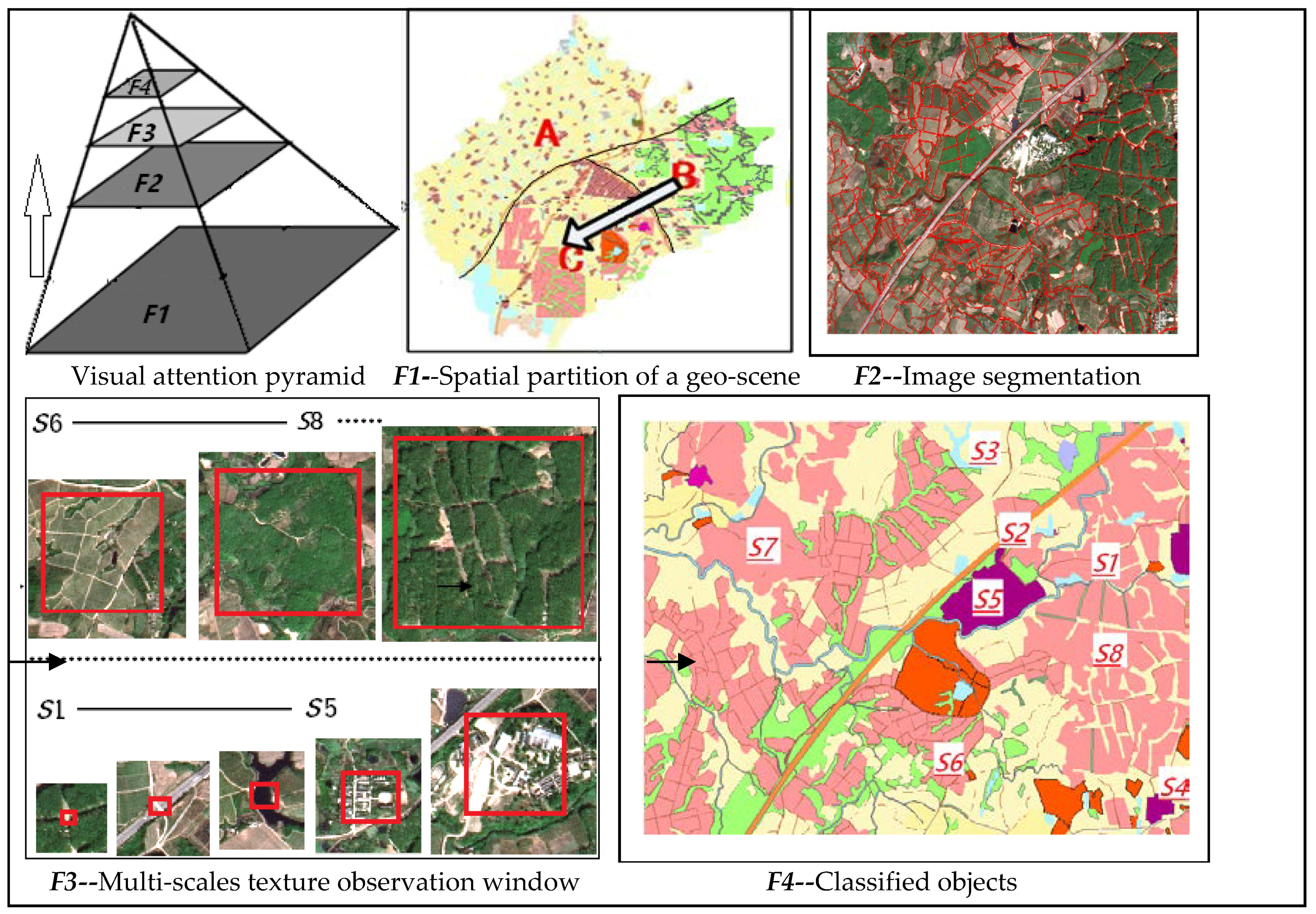
2. Overall Framework

GLCM is actually a statistical matrix of joint conditional probability distribution between the gray levels of image pixel pairs with some distance and direction within a certain window, and is used for texture descriptors [1,2,3]. Each geo-texture observation window based on GLCM must reflect the real spatial characteristics of the corresponding category. For example, in the classification system of land cover of I level, “woodlands” are taken as a single classified object. Thus, its texture unit is expanded, and a larger observation window and complex spatial structures are formed. In a classification system of land cover of II level, woodlands are subdivided into four sub-types: Dense woodland, Shrub woodland, Sparse land and other woodlands [31,32,33,48,49]. Obviously, for a texture unit of sub-types, its corresponding observation window should be relatively microscopic in the same place, and the spatial structure relatively simple. A case in which the classified geo-objects vary with the change of geo-classification system in an image can be seen in Figure 1.
In the geo-analysis of an image, each category should have its own texture observation window, which is strongly correlated with the actual definition and shape of the classified objects [20,21,22,23,24,25,26,27,28,29,30,31,32,33,34,35,36,37,38,39]. In addition, the scale selection algorithm is essentially equivalent to setting the image pixel number as the optimal scale according to the size of the object shape and the image resolution. Therefore, this paper uses GIS data and technology to mine domain knowledge (mainly the statistical characteristics of objects’ shapes), in order to determine the multi-scale of GLCM texture observation windows. The overall framework is designed as shown in Figure 2; the steps will be described below.
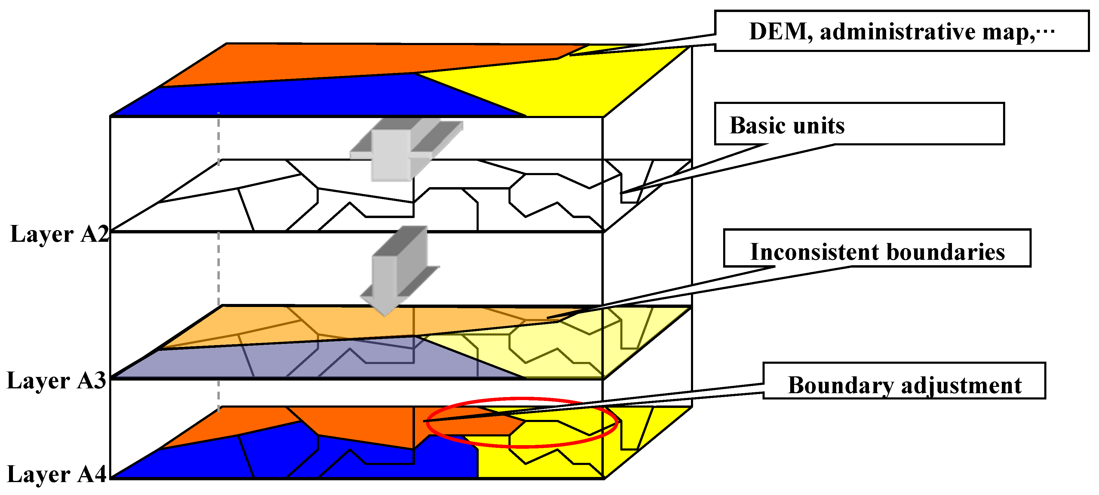
• Evaluating the validity of domain knowledge by spatial partitioning and image segmentation
The validity of the domain knowledge must be taken into account when using it to analyze texture windows. Because domain knowledge is mined from an existing GIS database, there is potential knowledge variability in the two time-phases, i.e., from GIS data to RS data. To obtain more effective domain knowledge and reduce the impact of such changes on the analysis results, some spatial data mining algorithms are employed, including spatial partitioning and image segmentation by GIS. The spatial partitioning can ensure the overall spatial consistency of a geo-scene, and the GIS-based image segmentation can further measure the stability of domain knowledge by analyzing the change rule of categories in segmentation blocks.
• Domain knowledge mining by GIS
In a stable time-space system, a set of effective polygons with representative shapes can be obtained from an existing GIS database, and the general shape characteristics of each category can be mined by employing GIS shape indices.
• Determination of multi-scale GLCM texture windows
According to the principle of determination, we set up a one-to-one model of the correlation between domain shape knowledge and texture scale to extract the appropriate multi-scale window for GLCM texture features.
• Evaluation of multi-scale parameters
To quantitatively evaluate the validity of texture scales extracted by GIS and domain knowledge, we employ the Fisher distance method, which can measure the separability of GLCM texture features under different scales; and the higher the separability, the better the setting of the corresponding scale parameters. First, a set of criteria for multi-scale parameters is obtained by measuring the separability of texture features based on enumerated scales. Then, the results deduced by the proposed method can be evaluated by means of a comparison analysis.
Overall, the progressive visual attention and cognitive process for the geo-texture scale in a geo-scene can be seen as “from the whole to the local, and from the window to the details” [21,45,46,47,48,49,50,51]. The process is illustrated in Figure 3:

3. Methods

3.1. Domain Shape Knowledge Mining by GIS

3.1.1. Spatial Partition

By considering various factors (including natural, social, and economic factors) that affect a certain geo-scene (such as the I level land-cover scene and II level land-cover scene, and the rural land-use scene and urban land-use scene, etc.), the original GIS data can be divided into several homogeneous pieces over a whole range. A partition piece can retain the pattern rules of a geo-scene, such as the consistency of natural landscape units, the consistency of ecological functions, the consistency of topology, or the integrity of administrative divisions [48,49,52]. The technology to achieve this process is referred to as spatial partitioning, including the overlay analysis method, the dominant factor method, the multi-factor comprehensive evaluation method and the cluster analysis method [52]. Based on a comprehensive comparison, this paper adopts the dominant factor method combined with the overlay analysis method, which considers the importance of various impact factors of a certain geo-scene and maintains the topology integrity and continuity of the region.
Specifically, we extract various factor layers for a certain geo-scene from existing GIS databases, such as digital elevation model (DEM) maps, administrative maps, main river maps, main road maps, etc., and then overlay polygons of these factor layers sequentially according to their importance. When the overlapping layer is inconsistent with the boundary of basic units (like a land-use polygon in a land-use scene), we adopt the maximum area principle to adjust the conflicting boundary (see Figure 4). Finally, we obtain a series of homogeneous partitioned regions for which the mined domain knowledge is basically consistent with that at the corresponding time of the GIS database.

3.1.2. Image Segmentation

In the partitioned region, above, the image segmentation blocks are obtained by cutting the RS image with the GIS basic unit data. Then, the frequency histogram for the mean gray value of segmentation blocks of each category is drawn in order to analyze the unchanged rate of each category within the two time-phases from GIS data to RS data, with the results indicating the degree of domain knowledge validity in this partitioned region.
First, the single-band image is calculated, instead of the original multi-band image, by using a classical dimension-reduction algorithm (e.g., principal component analysis or color space conversion), so that only one piece of gray value information is stored for each pixel, for efficient calculation. For a rough estimate of the validity of domain knowledge, the description of the grayscale image still reflects the combination information of bands, such as the color image. After the grayscale, the matrix dimension of the image is decreased, but the speed of operation is greatly improved, and the gradient information is still retained. Then, for category ω i , we use the frequency histogram to count the mean gray value of image segmentation blocks.
P s p e c t r u m ω i ( r k ) = n ω i k N s p e c t r u m ω i
In the equation above, r k is the k-th gray level of the image, expressed as the histogram abscissa. P s p e c t r u m ω i ( r k ) and n ω i k , respectively, indicate the frequency and numbers of the k-th gray that equals the mean gray value of the segmentation blocks of class ωi. P s p e c t r u m ω i ( r k ) is expressed as the histogram ordinate, and N s p e c t r u m ω i is the total number of segmentation blocks of category ωi.

3.1.3. Validity Evaluation of Domain Knowledge

We analyze the distribution characteristics of the above histograms of segmentation blocks in order to describe the validity of the knowledge.
In theory, if one of the above frequency histograms shows an obvious peak zone, then it indicates that the corresponding image segmentation blocks belong mainly to one category. Furthermore, if the category is the same as the historical one in the GIS database, then it indicates that these blocks have no significant changes in the land pattern between the two time phases. Assuming that the peak zone corresponds to the gray range as [ r ω i d o w n ,   r ω i u p ] , we can calculate the number of segmentation blocks that are not in the peak zone to quantify this changed rate V. As Yang C. and Zhou C. (2001) noted, if the proportion is less than the threshold value η, the time-space system is relatively stable, and it should satisfy the following formula [25]:
V ω i = ( 1 r k = r ω i d o w n r ω i u p p s p e c t r u m ω i ( r k ) ) × 100 % η

3.1.4. Shape Description

In a stable time-space system, the domain shape knowledge of a geo-scene can be strongly associated with the texture scale parameters. By comprehensively comparing various descriptive operators of the object shape, we adopt the minimum enclosing rectangle algorithm (MER). The MER refers to the minimum range that can contain a polygon’s shape, expressed in two-dimensional coordinates. The computation method comprises two main steps, one is to generate the enclosing rectangle (ER)—that is, set a rectangle under the polygon borders of the maximum abscissa, the minimum abscissa, the maximum ordinate, and the minimum ordinate. Then, the MER of a polygon can be obtained by rotating the polygon to the angle at which ER has the minimum area (see Figure 5). The MER is often used in GIS to give the approximate location and size of a geographic element. Many operations in GIS, such as spatial queries and spatial indexing, require the use of MER. Meanwhile, this operator has excellent performance when used to achieve RS image segmentation, and it can be a feature for aiding direct classification [30], because the MER adopts the minimum rectangular window with edges parallel to the axes to describe the polygon’s morphological characteristics, while GLCM also uses a rectangular window for texture feature description. Therefore, the MER window can directly describe the relationship between the polygon shape and texture scale.
First, we compute the MER of each polygon and record its parameters, including length and width, as {HER, WER}objID.
Next, the polygon regularity must be measured in order to judge whether it is suitable for shape knowledge mining. If the polygon’s shape is too narrow or curved, then the simple enclosing rectangle cannot describe its shape characteristics. In this paper, the rectangular-degree index is employed to achieve this measurement.
R = A / A M E R = A / ( H M E R × W M E R )
where A represents the actual area of a polygon and AMER represents its MER area. This indicator is simple and effective for the shape regularity description, and can reflect the degree to which a polygon fills its enclosing rectangle, as well as the irregularities of the polygon. The value of R is in the range from 0 to 1. R has a maximum value of 1.0 for rectangular objects, a value of π/4 for circular objects, and becomes smaller for objects with narrow, irregular, or curved shapes. If the rectangular degree of a polygon is lower, the texture characteristics under the MER window will be not accurate. Therefore, the following equation must be created to select the polygons with square-like shape for the subsequent analysis:
E s h a p e = { o b j I D | o b j I D { 1 , 2 , , N o b j } & & R o b j I D > T s h a p e }
In the equation above, N o b j represents the total number of polygons in the historical GIS database. R o b j I D represents the rectangular degree of polygon No. o b j I D . E s h a p e represents the polygon sets with regular shapes, wherein each polygon’s squareness degree is larger than the threshold value T s h a p e , as determined by the histogram method.

3.2. Multi-Scale Texture Window Determination Based on Domain Knowledge and GIS

3.2.1. One-To-One Associated Rules

Inspired by domain shape knowledge, texture scales can consequently be extracted; their associated rules are summarized as follows [31,32,33,34,35,36,37,38,39]:
  • A variety of categories should correspond to a variety of texture scales. This can be a one-to-one relationship or a many-to-one relationship. However, the number of texture scales should not be too large. Otherwise, it will cause information redundancy, increase algorithm consumption, and decrease the separability among the different categories. Therefore, the one-to-one model is chosen for analysis.
  • Each scale parameter can determine an observation window, which range should be close to, but slightly larger than, the polygon size of the classified object. If the window is too small, it cannot reflect the object’s spatial features. If the window is too large, the number of mixed pixels will be increased, resulting in spectral ambiguity and enormously reducing the classification accuracy.
  • If the classified object has a longitudinal structure (e.g., roads), it means that its width is relatively consistent, while its length and curvature are often uncertain. Therefore, we would choose an observation window related to the structure’s width.

3.2.2. Scale Determination

According to the one-to-one model, we can obtain the scale parameter for each category from the regular polygon collection E s h a p e by analyzing the frequency histograms of the polygon shape. Assuming that N ω i is the total number of regular polygons of the category ω i , then the frequency histogram of MER length can be defined as the following discrete function:
P ω i l e n g t h ( S ) = n ω i l e n g t h N ω i
In this frequency histogram, S represents the ranges of MER length of the category ω i , and ordinate n ω i l e n g t h and P ω i l e n g t h ( S ) , respectively, represent the number and probability of the polygons that are distributed in the range S. Additionally, the frequency histograms of the rectangular width P ω i w i d t h ( S ) will be similarly drawn.
In theory, if a category has similar shape for its polygons, then there should be a peak region distributed in its shape frequency histogram, above, whereby the corresponding shape size is able to cover the majority of polygons of this category and to achieve valid texture observation.
According to the selection principles, among the peak data of the MER length and width, if the larger one is chosen, the texture observation window will contain too many mixed pixels, thus reducing the feature validity, so it is easier to choose the smaller of the two values as the observation window of GLCM texture for this category. In this paper, the scale parameter is defined as half the number of image pixels corresponding to the observation window in geo space. Therefore, the final scale value should be divided by double the pixel resolution of an image, that is, pResolution × 2, as in the following equation:
S c a l e i = min ( w i d t h S c a l e i , l e n g t h S c a l e i ) / ( pResolution × 2 )
In this way, the best scale for the GLCM texture of each category will be obtained.

3.3. GLCM Texture Feature Evaluation Based on Fisher Function

3.3.1. GLCM Texture Features Based on Multi-Scales

GLCM is a matrix that is defined by the following parameters: observation window scale, distance and direction of pixel pairs, band and gray level of distribution probability. Since this paper mainly discusses the influence and performance of texture scale parameters on the separability of categories, the other parameters for GLCM construction have been selected using conventional and common ways. In fact, 14 kinds of GLCM-based texture feature have been defined, and 8 kinds of classical feature are commonly used for RS image analysis. They are {mean, variance, homogeneity, contrast, dissimilarity, entropy, angular second moment, and correlation} [2,3,31,32]. Therefore, these 8 texture features are also used for our experiments.
In this way, for a pixel k , its texture features set based on the scale s c a l e i is denoted as x k ( i ) . Then, all the texture features can be expressed as a feature vector t e x t u r e F e a t with dimension of K × M (where K is the number of pixels, and M is the number of scales and categories), as shown in Equation (7).
t e x t u r e F e a t = [ x 1 ( 1 ) , x 1 ( 2 ) , , x 1 ( M ) x 2 ( 1 ) , x 2 ( 2 ) , , x 2 ( M ) x k ( i ) x K ( 1 ) , x K ( 2 ) , , x K ( M ) ]

3.3.2. Separability Evaluation

Extracting multi-scale windows for texture features is better able to distinguish different categories from an image. Therefore, a quantitative criterion for measuring the validity of these texture features for classification should be employed. In general, different categories can be distinguished because they are located in different regions of the feature space. Obviously, a smaller or no overlap of these regions indicates better separability of features, as expressed in Figure 6.
The criteria for class separability evaluation commonly include Euclidean distance, Fisher distance, K-L distance, and others. In complex image classification situations, the Fisher distance adopts the determinant ratio of the between-class scatter matrix and the in-class scatter matrix as the separability criterion. Therefore, it can take the overall and local distribution characteristics into account. This method has performed well in traditional studies [44,45,46,47]. Thus, it has also been used to evaluate the validity of texture features in various scales in this study.
Specifically, x k ( i ) and x k ( j ) denote the eigenvectors of categories ω i and ω i , respectively. Then, the average distance between eigenvectors of categories is defined as Equation (8):
d ¯ ( x ) = 1 2 i = 1 M P i j = 1 M P j 1 N i N j k = 1 N i k = 1 N j d ( x k ( i ) , x k ( j ) )
In the above formula, P i and P j , respectively, represent the a priori probabilities of the corresponding categories, which can usually be expressed on the basis of probabilistic statistics of the samples in each category. Assuming that the number of sample pixels of category ω i is N p i , then P i can be obtained by Equation (9):
P i = N p i i = 1 M N p i
In addition, d ( x k ( i ) , x k ( j ) ) denotes the Euclidean distance between x k ( i ) and x k ( j ) . This is defined as Equation (10):
d ( x k ( i ) , x k ( j ) ) = [ ( x k ( i ) x k ( j ) ) T ( x k ( i ) x k ( j ) ) ] 1 2
Then, the overall in-class scatter matrix of samples can be defined as Equation (11):
S w = i = 1 M P i 1 N p i k = 1 N p i ( x k ( i ) m i ) ( x k ( i ) m j ) T
The overall between-class scatter matrix of samples can be defined as Equation (12):
S b = i = 1 M P i ( m i m ) ( m i m ) T
The overall scatter matrix of samples can be defined as Equation (13):
S t = 1 i = 1 M N p i i = 1 M ( x i m ) ( x i m ) T
In the above formula, m i represents the average feature space vector of samples in category ω i and m represents the average feature space vector of samples of all categories. These are defined as Equation (14):
m i = 1 N p i i = 1 N p i x k ( i ) ,   m = i = 1 M P i m i
Then, the criteria for separability of categories can be defined as Equation (15):
a = 1 , J = d 2 ( x ) = T r [ S w + S b ] = T r [ S t ]
In the above formula, Tr {.} represents the trace of the matrix (the sum of the diagonal elements of the matrix). In this way, the trace of the overall scatter matrix of samples (the Fisher distance) can be used as the separability criterion. The larger the value, the more dispersed the samples and the better the separability.

4. Experiment and Discussion

4.1. Study Data

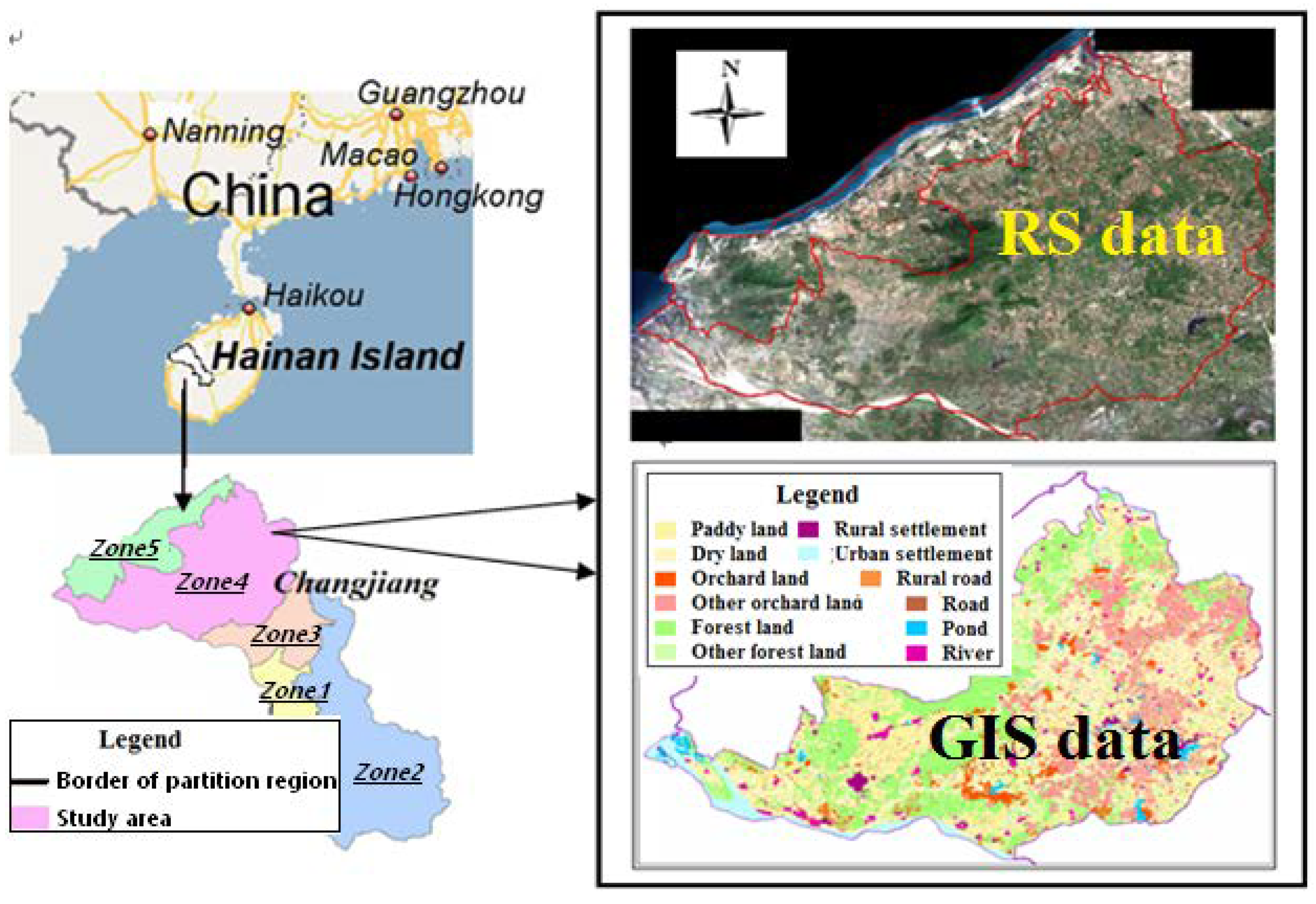
In this paper, Changjiang County, Hainan Province was chosen as the study area. We aimed to obtain effective scale parameters for multi-scale GLCM texture features in distinguishing the land-use categories. Land-use classification is a common geo-scene in practical work, with a complex system and specific meaning. The collected study data include the following. (1) The 2008 SPOT5 RS image, which has a high spatial resolution of 2.5 m and a true color space (Red, Green, Blue). It is intended for land-use classification cartography of 1:10,000. (2) The existing GIS database in vector format, including 2005 and 2008 GIS land-use maps at the scale of 1:10,000, where the 2005 GIS data can be used to extract domain knowledge, and the 2008 GIS data can be taken as the current real geo-objects to verify the classification accuracy. The other auxiliary GIS data, which are mainly used for spatial partitioning, include the 2006–2020 land-use planning map and DEM graded map, etc.

4.2. Spatial Partition and Classification System of Land-Use

First, by using the 2006–2020 GIS and land-use planning data, we extract the following partitioning factors: important resource distributions, administrative boundaries, and the functional division map. Meanwhile, the 2005 land-use polygon boundary is taken as the basic unit. Their cartographic priority is set according to the visual size in the local region as follows: DEM graded map > railway distribution map > provincial and municipal highway distribution map > important river distribution map > functional division map > village administrative boundary map. According to this order, each factor map should be superimposed on the basic land-use polygon. Finally, the study area is divided into five homogeneous regions, which have to maintain the integrity and continuity of land-use polygons and administrative boundary, as shown in Figure 7.
According to land-use planning, the land-use pattern of the Zones 2–4 will not be extensively adjusted in 2005–2008, so the domain knowledge mined from the 2005 land-use map in these regions is seen to be usable. To better illustrate the adaptability of the proposed method, the 4′ Zone has been chosen for the experiments because it has a more complex land-use pattern.
According to the latest land-use classification system used in practical work, there should be 12 land-use classification categories (see in Table 1).

4.3. Evaluation of Domain Knowledge

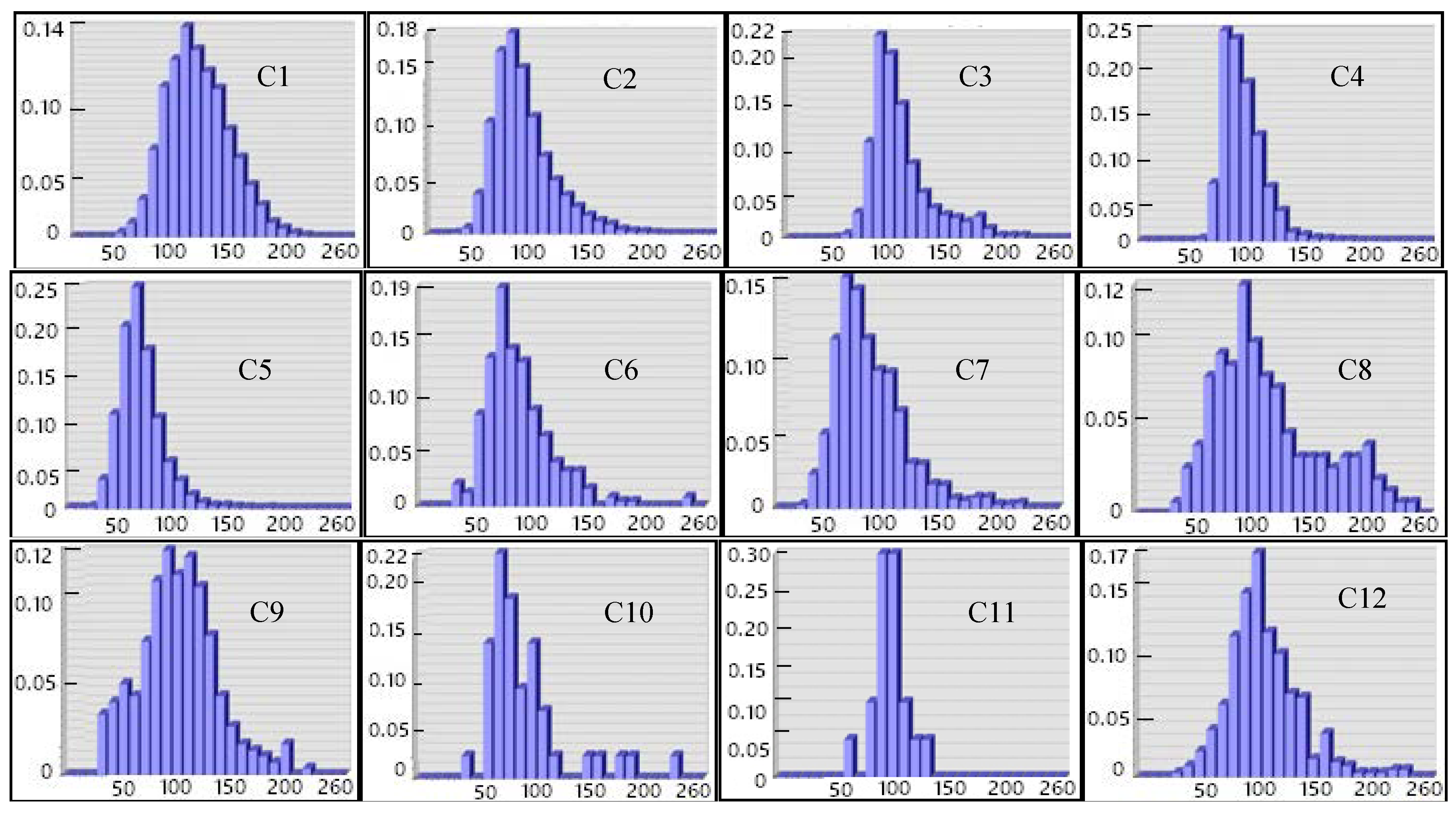
In the ArcGIS software, we first split up the RS raster image using the GIS vector polygon boundary and calculate the mean gray value of each segmentation block. For this RS image with 3 bands, its gray image can be obtained by converting color space from RGB (red, green, blue) to HSI (hue, saturation, and luminance) and eliminating the hue and saturation information while retaining the luminance values. When we plot the frequency histograms of the blocks under the corresponding gray levels of each category, the gray level is set as 26, which means that there are 26 breaks/bars in the histogram, i.e., rk = 1, 2, …, 26, and each level is 10. Since the category number is 12, we get 12 groups of statistical graphs of the gray level of segmentation blocks, as shown in Figure 8:
Thus, we can easily obtain the peak zone of a histogram above because of its approximate normal distribution. Then, Equation (2) will be used to count the changed-rate V of the number of polygons for each category. The statistics are shown in Table 2, where the total number of polygons of each category in the historical GIS data is denoted as totNum, and the number of polygons for which the category has not been changed between the two-time phases is denoted as tipNum. Following related previous works (especially by Yang C., Zhou C. 2001), in the classical statistical theories of the “golden section” and “five-grade marking”, the changed rate of polygons’ number of a category should be lower than the threshold η as 40%; that is, at least 60% of the polygons’ categories should not have been changed. In this case, the domain knowledge system can be characterized as stable and qualified [25,48,49].
In the table above, a smaller polygon category’s changed-rate results in higher stability. Because most categories meet the pre-defined judgment of Equation (2), they are relatively stable and unified under the selected spatial-time scale in which the corresponding domain knowledge is reliable. Meanwhile, the changed-rate of categories 8 and 10 are near 40%. Therefore, that corresponding domain knowledge may be relatively ineffective in the subsequent analysis.

4.4. Scales Determined by GIS and Domain Knowledge

Based on the secondary development program function of the ArcGIS platform, the following operators have been obtained.
(1)
There are a total of 17,991 land-use polygons in the partition region, of which 3893 patches were selected according to their regularity as effective polygon shapes for morphological knowledge statistics.
(2)
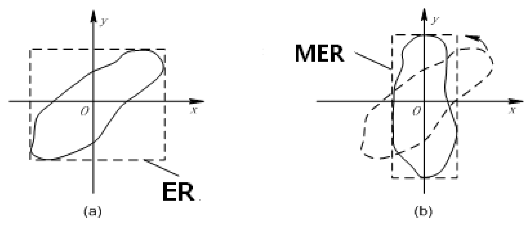
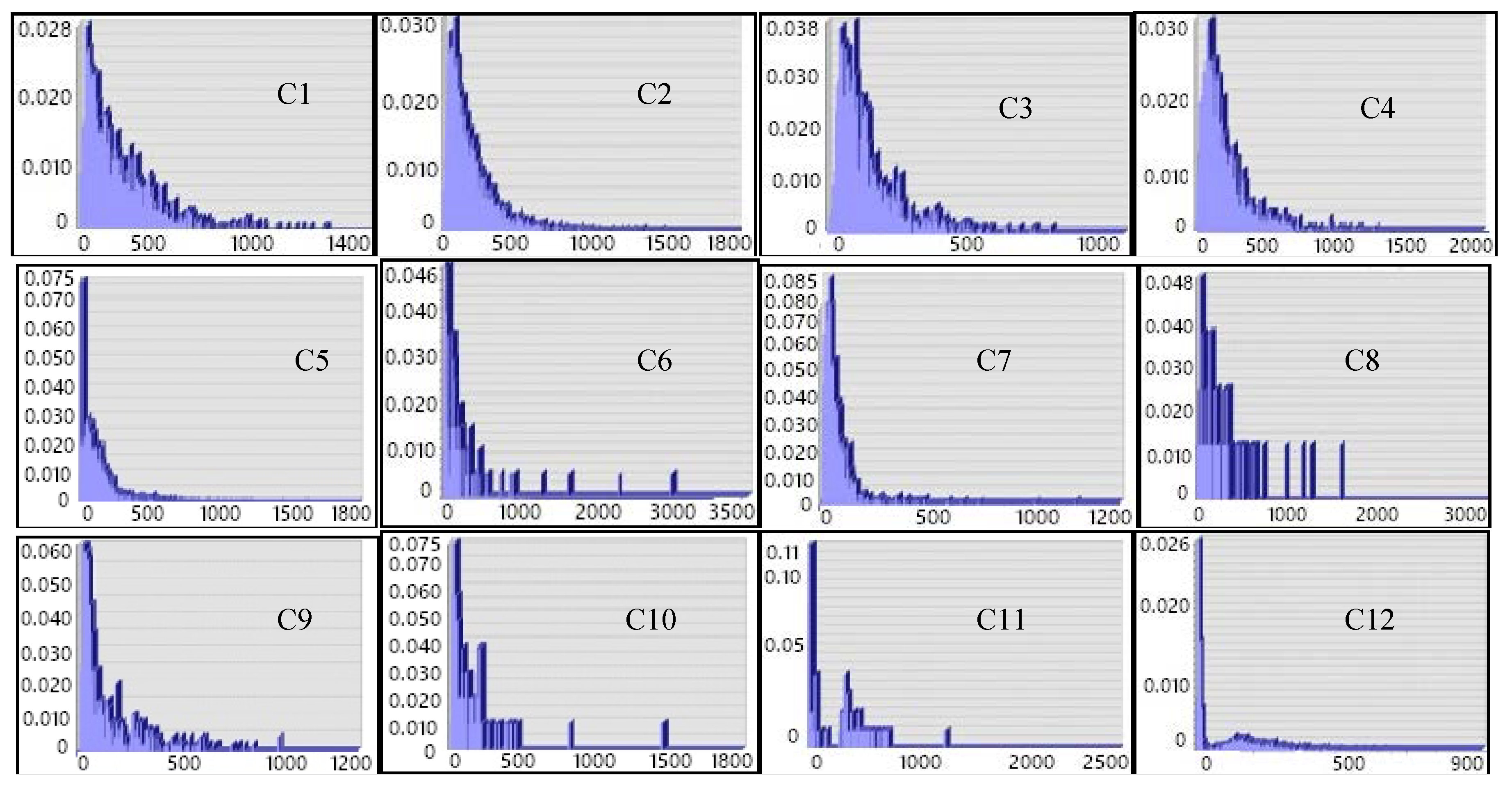
According to the effective polygon sets, we plot out the frequency histograms of the length and width of the MER for each category. Because we are interested only in the shorter side of the rectangle, as described in the discussion and Equation (6) above, frequency histograms of the widths of MER should be plotted for each category, as shown in Figure 9.
These figures show the following rules. (1) There are obvious peaks in most categories, which shows that a strong regularity lies in their morphology. Moreover, a more concentrated frequency distribution indicates a more obvious morphological regularity with its category. (2) There is no obvious peak or peaks in a few categories. This includes category 8, which contains several morphological characteristics. Therefore, the validity of their domain knowledge has been further constrained.
(3)
The texture scale parameter Scalei of each category is set by selecting the smaller value of the statistical width and length of MER, in accordance with Equation (6). Meanwhile, we indicate the variance of the length and width as STD_Width and STD_Length to measure the representativeness of the selected texture scale. Then, the scale value should be the nearest odd number obtained by the window size in geo-space divided by pixel resolution × 2 (2.5 × 2 = 5 m in this study). The results are shown in Table 3.
According to the analysis in Table 3, some conclusions can be obtained. (1) The minimum texture scale corresponds to category 12 (rural road). It is a linear feature that takes the line width as a basis for analysis. The maximum texture scale corresponds to category 8 (river), which has the largest area and an irregular shape. At the same time, however, we should also note that there are still some short and small rivers in the study area. The texture features observed on this large a scale are not conducive to the extraction of these objects. For categories 1–6 (a series of cultivated lands), the selected texture scales are also larger, which indicates that there is a massive stretched distribution in the polygons. This conclusion can also be directly observed from the GIS historical database. Moreover, category 9 represents a rural residence, and its texture scale is much smaller than the urban residence in category 10. This result is also in accordance with the actual case. (2) The variances in the length and width of the enclosing rectangles for most categories are generally less than 50, except for category 8, which has a variance greater than 70. This result further illustrates that the differences in the morphological characteristics of category 8 will lead to a consequence of there beingno representative scale that can be selected.
In conclusion, the texture scale sets that are selected with the aid of GIS historical knowledge are in accordance with the local actual situation and people’s general cognition.

4.5. Scales Determined by the Enumeration Method

In this paper, the Fisher distance algorithm is employed to quantitatively measure the validity of the selected texture scales. The determinant ratio of the between-class scatter matrix and the within-class scatter matrix has been taken as the criterion of category separability in this index.
(1)
First, the enumeration method is used to calculate texture features under a series of scales. On the basis of relevant research results [31,32,33,34,35,36,37,38,39,40,41,42], we select an enumeration scale of L = 3:101.
As for setting the other parameters of GLCM-based texture features, some conventional and efficient methods were used (as shown in Table 4), with the single-band image value also being obtained by converting the color space from RGB to HSI and retaining the luminance values of HSI, thereby obtaining the distance value that is most commonly set to 1, and obtaining the direction value by computing the average texture statistics in its four directions. Additionally, the dimension of GLCM is determined by the image gray level. Considering the calculation efficiency and the storage need of the matrix in practical applications, the gray level of the original image should be compressed, i.e., an 8-bit image with a gray level of 0–255 is compressed into a 3-bit image with a gray level of 0–8, which can effectively avoid the sparse matrices in GLCM.
In this way, we can calculate 8 classic GLCM-based texture features as described in Section 3.3.1; meanwhile, we employ a principal component analysis algorithm to deduce 3 principal features, so as to reduce feature dimensions and ensure their independence. These two groups of texture features with number of 8 and 3 are denoted as I and II.
(2)
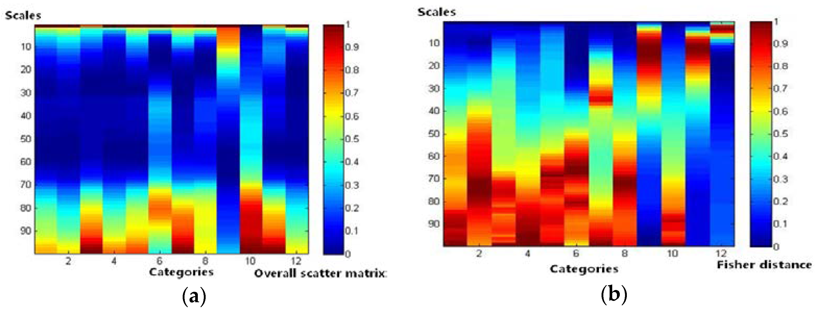
Second, the Fisher distances of the two groups of texture features based on the enumeration method are computed. In the following relational diagram, we define the category number as the x-axis and the texture scale as the y-axis. We also describe the value of the overall scatter matrix and the Fisher distance using different color blocks. Blue represents the smallest separability, and red represents the largest separability. Therefore, the relationship between the category separability and the texture scales can be clearly expressed.
The results are shown in Figure 10. Group I of the overall scatter matrix and Fisher distance is derived under 8 texture features, while the group II of the overall scatter matrix and Fisher distance is derived under 3 independent texture features. It can be observed from these graphs that: (1) For the overall scatter matrix, the peak value is distributed in a more concentrated way and is more inconsistent in all categories in group I than in group II. In addition, most categories reach high separability on some slightly smaller scale values in group II than in group I. This illustrates that, when the texture features are more independent, the separability of all categories is more consistent and can be obtained on a smaller scale value. (2) For the Fisher distance, in any category (column), there is always a peak zone in the separability bar chart, and the separability of such zone changes mostly scales according to the normal distribution, and it fluctuates. The peak values of each category in group I and group II are close. However, fluctuations and noise occur occasionally in group I, such as in category 6, while the peak region has a more obvious and concentrated distribution in group II. This illustrates that the separability is more prominent and clear when the texture features are more independent, and vice versa.
In addition, it should be noted that most categories with complex texture features or mixed pixels can be separated under a bigger texture scale value; that is to say, if only one scale parameter can be used to calculate the texture features in a particular case, its value should be as large as possible.
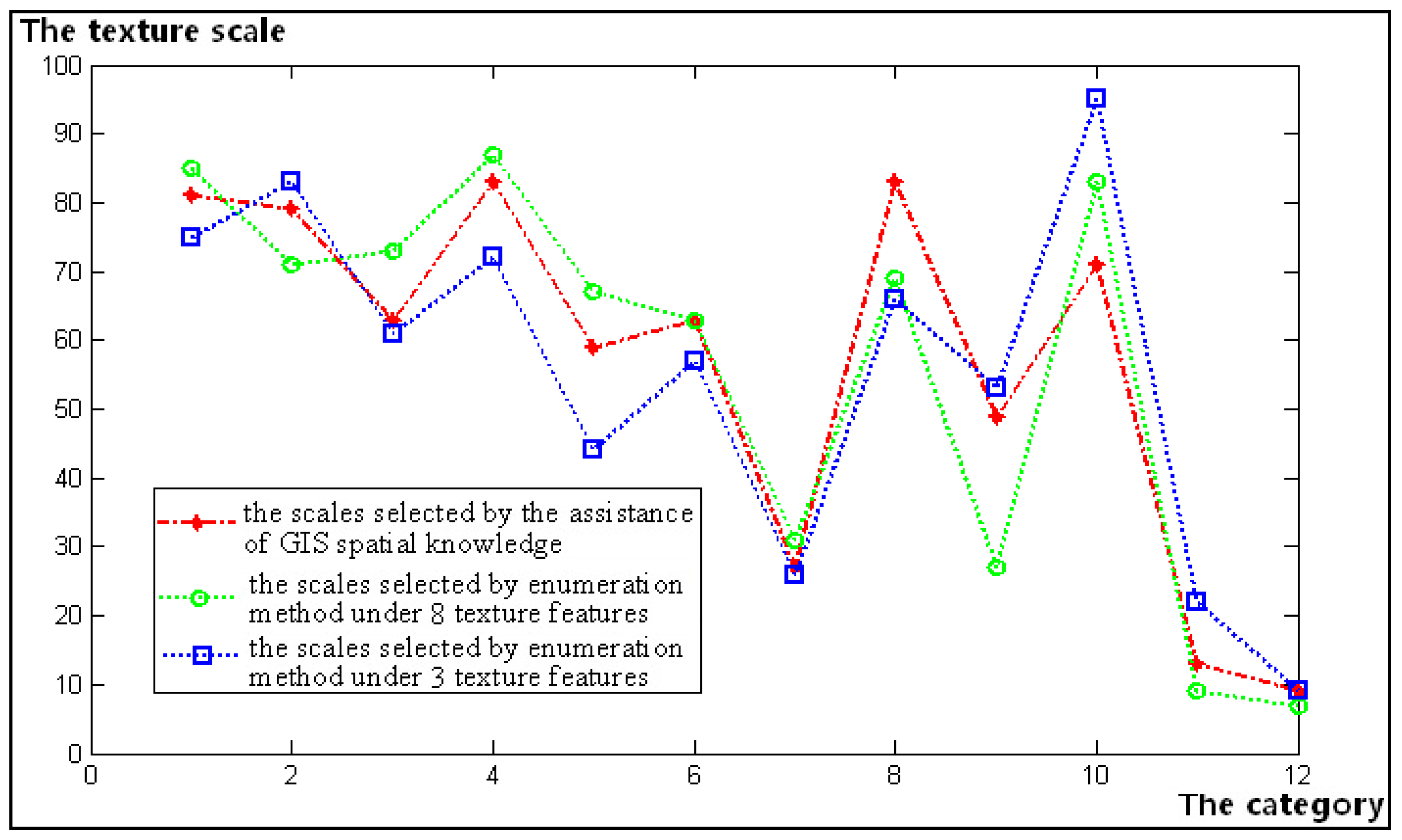
As a result, the scales corresponding to the highest separability of each category were computed. The texture scale sets determined by the different methods can be seen in Table 5.

4.6. Comparison of the Different Scale Sets

For the three groups of texture scale sets shown in Table 5, the relationship among them can be summarized as shown in Figure 11.
Some conclusions can be reached.
(1)
Intuitively, the scales that are selected by the different methods are very close and even have the same values in some categories. However, there is also a larger difference between categories 8 and 10. By analyzing the cause of the divergence, we find that category 8 represents river water, whose shape is larger in the GIS historical database. Therefore, the texture scale that is determined by its domain knowledge has a larger value of 83. However, significant changes have occurred in this category within two time-phases (see Table 1, with the change rate of 41.1%), because many rivers continue to diminish, and the standard scale parameter that is determined by the enumeration method has a smaller value of 69 or 66. Moreover, similar to category 10 (urban settlement), the scale that is determined with the aid of the GIS historical data is 71, but the standard texture scale that is determined by the enumeration method has increased to 83 or 95 with the continuous expansion of the town over several years. Therefore, under this unstable cognitive spatial-temporal system, the reliability of its domain knowledge is greatly reduced. In the scale sets 2 and 3, which are selected by the enumeration method, we can generally gain a smaller value in set 3 for most categories under 3 independent texture features. This shows that, under the same distinguishing performance, the independent texture features can slightly reduce the window scale value for texture observation in most instances.
(2)
The correlation of the different texture scale sets was computed, as seen in Table 6.
The calculation results show that the relativity Re reaches 0.93, and the significance p reaches 0.00075 in the first group of scale sets, while the relativity Re reaches 0.91, and the significance p reaches 0.00039 in the second group of scale sets. The closer the Re value is to 1, the higher the relativity between the two sets of data is; and the further the p value is below 0.05, the more significant the correlation is. Although the relativity value in the second group is slightly worse than that of the first group, its significance value is better. It is reaffirmed that the increase in the independence of the texture features enables a more significant and clear value of the scale sets derived, while the scale sets also maintain a strong performance.

4.7. Classification Results Analysis

To further evaluate the proposed method for setting texture scale sets, we carried out an experiment comparing classification ability. The SVM algorithm was employed. As a classic method, it has performed well in image analysis in many studies [1]. Specifically, we achieved image classification by using GLCM-based texture features under a series of typical single- or multi-scale sets.
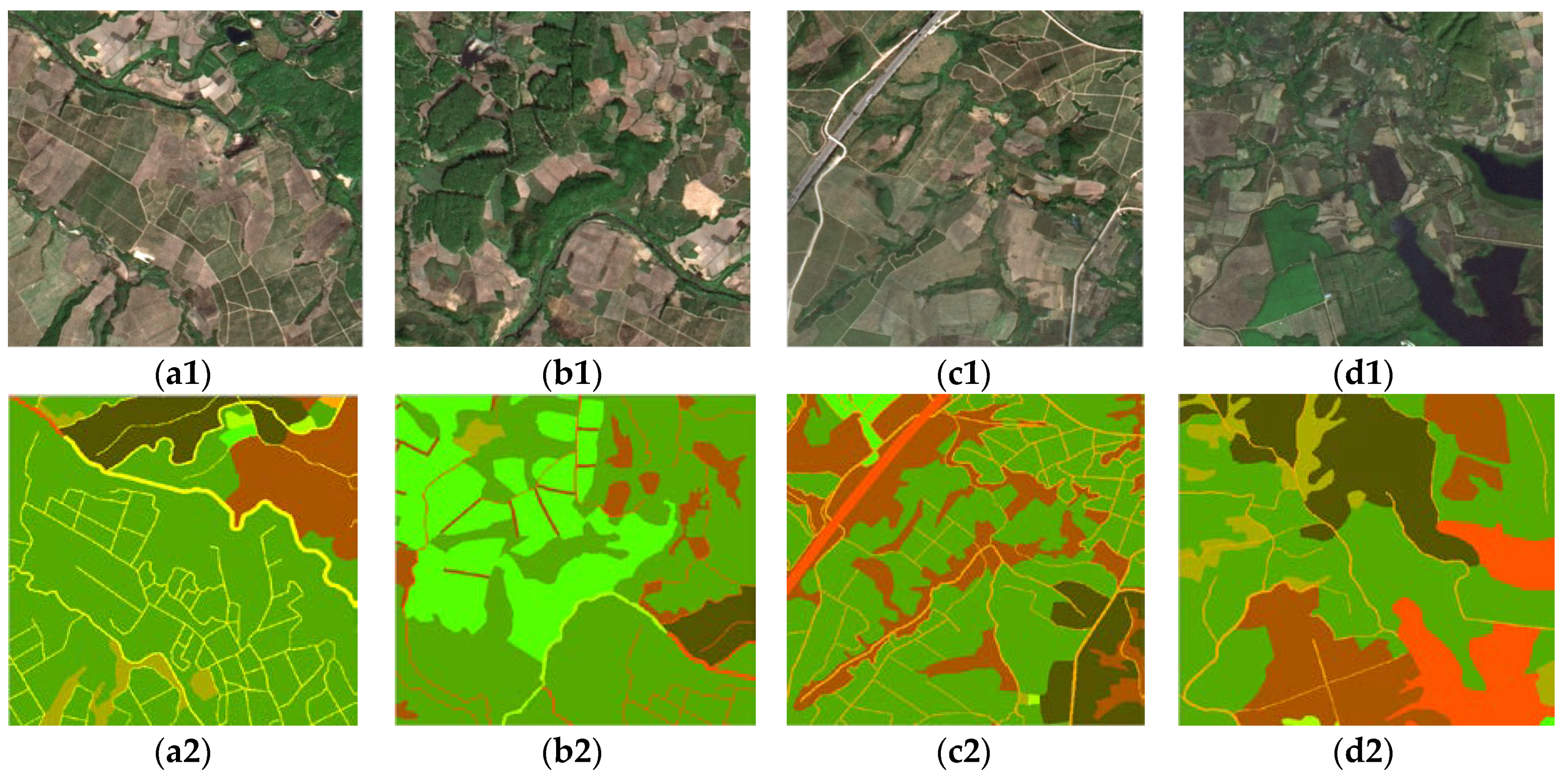
First, we choose any images cut from the RS data in the study area (as shown in Figure 7) for testing. The size of each cut image is 500 × 500 pixels, and its classification system is as shown in Table 7 and Figure 12.
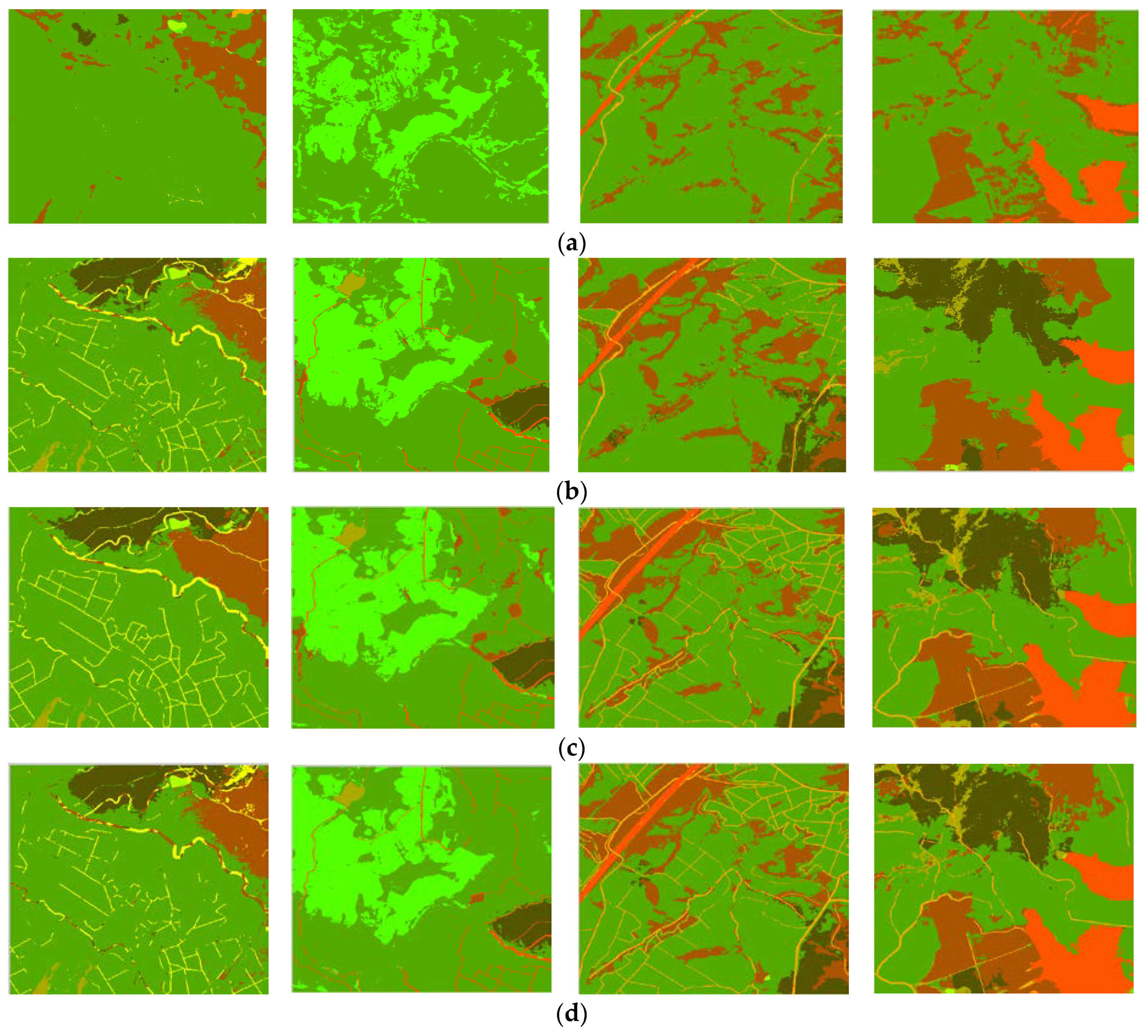
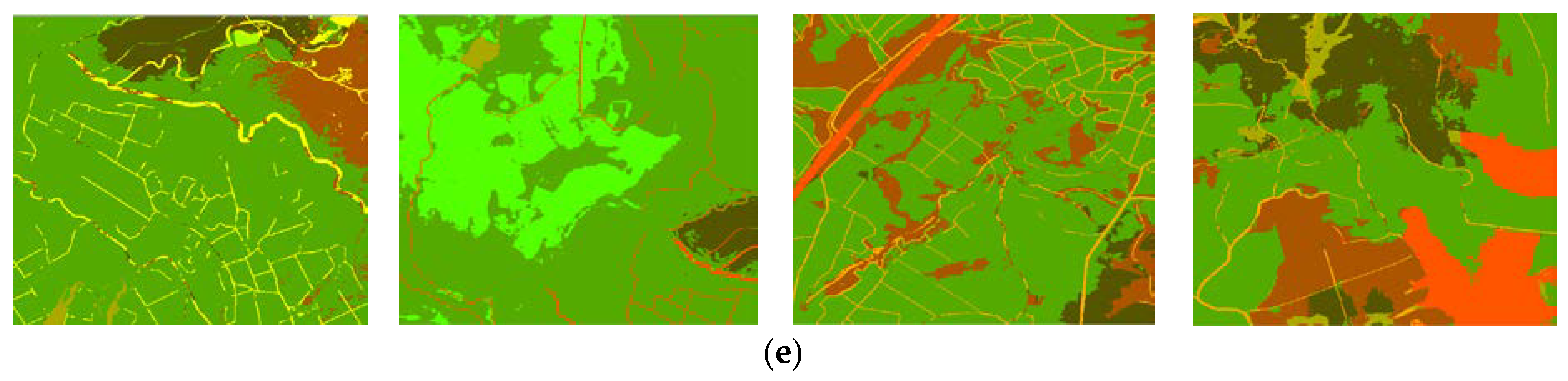
Then, the sample ratio parameter is set as 0.3, 0.6, or 0.8, while the other parameters remain unchanged from the SVM algorithm. Since the variation in classification accuracy is within 1%, its influence on the algorithm can be regarded as negligible. Therefore, we use the sample ratio of 0.3, in consideration of algorithm efficiency. The experiments results are as shown in Figure 13.
The overall accuracy and kappa coefficient are calculated in Table 7.
As shown in the results above, the classification abilities of different feature spaces are as follows: the classification accuracy is lowest when only spectral features are used, followed by the integrated usage of texture features under a single scale, and the highest accuracy, especially the highest kappa coefficient, is from the integrated usage of texture features under multi-scale sets.
When the single-scale value is gradually increased from 1, the overall classification accuracy significantly increases and reaches the highest level when the scale value, respectively, is 89, 81, 79, 73 in image 1–4. When the multi-scale is respectively given as sets 1, sets 2, and sets 3, the classification accuracy are all high value and very close in images 1–4. However, the optimal scale sets is different for these different classification systems, that is to say, no a kind of scale sets has absolute classification advantage. Overall, there are strong and significant correlations between the 3 groups of scale sets, which further proves the rationality and validity of the proposed method that extracts the texture scale based on domain knowledge and GIS.

4.8. Algorithm Efficiency Analysis

(1)
With the enumeration method, the best scale parameters can be gained by comparing texture features under numerous scales. When the range of the enumerated scale was set from 3 to 111 in this experiment, the algorithm’s time consumption changed, as shown in Figure 14a.
Clearly, this algorithm is extremely time-consuming. As the texture scale increases, the time consumption for calculating texture features increases exponentially. When the scale is larger than 15, the time consumption exceeds 10 min, with the maximum even reaching 5 h (i.e., when scale = 111). If the enumeration method is used to determine texture scale parameters, as the image data continues to increase, the accumulated time will reach an unbearable degree, such as in Equation (16):
y = i = 1 m a x E N k 1 e ax i
The equation above is derived from the exponential regression line in this study, where k1 and a are the variables determined by the computer’s performance, and maxEN represents the maximum value of the enumeration number. It shows that algorithm complexity is a relationship of cumulative exponential regression.
(2)
Based on the GIS and the domain knowledge-assisted method, the texture scale features can also be effectively extracted. This is realized through traversal, statistics, and the analysis of patches from the existing GIS database using the ArcGIS platform. When the proposed method is widely used, and GIS data can be managed in a standardized way, then its algorithmic complexity will be largely proportional to the number of patches. The corresponding time consumption can be reflected in the following statistical curve in Figure 14b.
It can be seen that this algorithm has superior performance, especially in terms of efficiency. It only takes 180 s to perform the operation on the entire experimental area (region 4 of size 581 km2). Therefore, compared with the enumeration method, it substantially increases efficiency and is therefore more suitable for high-resolution remote sensing image analysis of larger geo-data. We summarize the relationship between polygon numbers and time consumption in Equation (17):
y = b + k 2 x
The equation shows a simple linear relationship, where b is the time of data management and data cleansing of GIS, and k2 is the variable determined by the computer’s performance. The algorithm has very low complexity; moreover, the calculation results are reasonable and valid, which is consistent with the scales selected by the enumeration method. It can be said that the texture scale extraction method based on the spatial knowledge of land-use proposed in this paper is scientific and reasonable and can meet the efficiency and precision requirements of classification.

5. Conclusions

  • In a geo-scene classification of high-resolution RS images based on GLCM texture, the window scale of GLCM is an important parameter for determining its validity. Since the classification system changes with different needs, the observation windows of GLCM should also be changed correspondingly, so that the real texture features of classified objects can be intuitively reflected. Based on this, a one-to-one model that is strongly correlated with the actual definition and shape of classified objects was built to set the texture scales of each category. This is a new and practical method that is easy to understand and use.
  • The proposed approach is based on the integrated computation of existing GIS data and current RS data, and the comprehensive use of a variety of domain shape knowledge, thereby avoiding the disadvantages of local optimum, sample dependence, and initial error accumulation when compared with other approaches relying only on the images themselves. Moreover, it shows a significant improvement in efficiency.
  • In terms of the experimental results, the multi-scale value keeps the one-to-one relationship with the classified objects, and their value ranges are from a few to tens, rather than the smaller values of traditional analysis. Since most categories with complex texture features or mixed pixels are separable under bigger texture scales, the GLCM texture descriptors under these geo multi-scale windows can evidently represent the different geo categories. Meanwhile, the proposed approach has good performance that is the same as the classical enumeration approach and high calculation efficiency, so it can not only increase the total number of categories for a certain geo-scene, but also reduce the classification uncertainty. Obviously, the integrated use of RS image spatial features and GIS domain knowledge is proved necessary and effective in image geo-texture analysis.
Future research will construct a united platform in order to collectively handle and analyze the GIS and RS statistics and further contribute to the selection of the GLCM texture direction with the aid of GIS and domain knowledge.

Author Contributions

Z.L. provided the initial idea for this study, conceived the experiments, and wrote the paper; Y.L. contributed the experimental data and supplied the infrastructure for the experiments; and Z.L. and Y.L. performed the experiments and analyzed the results.

Funding

This research was funded by National Natural Science Foundation of China(NSFC) grant number 4130137.

Acknowledgments

This paper was also received the help from B.J., M.Y., and Y.C., et al., in Guangzhou Urban Planning & Design Survey Research Institute. They provided important suggestions and reviews.

Conflicts of Interest

The authors declare no conflicts of interest.

References

  1. Lu, D.; Weng, Q. A survey of image classification methods and techniques for improving classification performance. Int. J. Remote Sens. 2007, 28, 823–870. [Google Scholar] [CrossRef]
  2. Liu, X. Summary of texture Research. Appl. Res. Comput. 2008, 25, 2284–2288. [Google Scholar]
  3. Haralick, R.M.; Shanmugam, K.; Dinstein, R. Textural features for image classification. IEEE Tran. Syst. Man Cybern. 1973, 3, 610–621. [Google Scholar] [CrossRef]
  4. Gong, P.; Howarth, P.J. Frequency-based contextual classification and gray-level vector reduction for land-use identification. Photogramm. Eng. Remote Sens. 1992, 58, 423–437. [Google Scholar]
  5. Randen, T.; Husoy, J. Filtering for Texture Classification: A Comparative Study. IEEE Trans. Pattern Anal. Mach. Intell. 1999, 21, 291–310. [Google Scholar] [CrossRef]
  6. Manjunath, B.S.; Ma, W.Y. Texture Features for Browsing and Retrieval of Image Data. IEEE Trans. Pattern Anal. Mach. Intell. 1996, 18, 837–842. [Google Scholar] [CrossRef]
  7. Reyes-Aldasoro, C.C.; Bhalerao, A. The Bhattacharyya space for feature selection and its application to texture segmentation. Pattern Recognit. 2006, 39, 812–826. [Google Scholar] [CrossRef]
  8. Malpica, N.; Ortuño, J.E.; Santos, A. A multi-channel watershed-based algorithm for supervised texture segmentation. Pattern Recognit. Lett. 2003, 24, 1545–1554. [Google Scholar] [CrossRef]
  9. Trevisani, S.; Rocca, M. MAD: Robust image texture analysis for applications in high resolution geomorphometry. Comput. Geosci. 2015, 81, 78–92. [Google Scholar] [CrossRef]
  10. Guo, Z.; Zhang, L.; Zhang, D. Rotation invariant texture classification using LBP variance (LBPV) with global matching. Pattern Recognit. 2010, 43, 706–719. [Google Scholar] [CrossRef]
  11. Atkinson, P.M.; Lewis, P. Geostatistical classification for remote sensing: An introduction. Comput. Geosci. 2000, 26, 361–371. [Google Scholar] [CrossRef]
  12. Herzfeld, U.C. Master of the obscure—Automated geostatistical classification in presence of complex geophysical processes. Math. Geosci. 2008, 40, 587–618. [Google Scholar] [CrossRef]
  13. Chica-Olmo, M.; Abarca-Hernandez, F. Computing geostatistical image texture for remotely sensed data classification. Comput. Geosci. 2000, 26, 373–383. [Google Scholar] [CrossRef]
  14. Zhang, C.; Franklin, S.E.; Wulder, M.A. Geostatistical and texture analysis of airborne-acquired images used in forest classification. Int. J. Remote Sens. 2004, 25, 859–865. [Google Scholar] [CrossRef]
  15. Lucieer, A.; Stein, A. Texture-based landform segmentation of LiDAR imagery. Int. J. Appl. Earth Obs. Geoinf. 2005, 6, 261–270. [Google Scholar] [CrossRef]
  16. Qian, X.; Hua, X.S.; Chen, P. An effective local binary patterns texture descriptor with pyramid representation. Pattern Recognit. 2011, 44, 2502–2515. [Google Scholar] [CrossRef]
  17. Ojala, T.; Pietikäinen, M.; Mäenpää, T. Multi-resolution gray-scale and rotation invariant texture classification with Local Binary Patterns. IEEE Trans. Pattern Anal. Mach. Intell. 2002, 24, 971–987. [Google Scholar] [CrossRef]
  18. Zhu, C.; Wang, R. Local multiple patterns based multi-resolution gray-scale and rotation invariant texture classification. Inf. Sci. 2012, 187, 93–108. [Google Scholar] [CrossRef]
  19. Qin, Q. Problems in Automatic Interpretation of Remote Sensing Images and Ways to Solve. Sci. Technol. Surv. Mapp. 2000, 25, 21–25. [Google Scholar]
  20. Chen, Z. Research on High-Resolution Remote Sensing Image Classification Technology. Ph.D. Thesis, Institute of Remote Sensing Applications, Chinese Academy of Sciences, Beijing, China, 2006. (In Chinese). [Google Scholar]
  21. Chen, S. Geo-spatial/temporal Analysis in Geo-processing. J. Remote Sens. 1997, 1, 161–169. (In Chinese) [Google Scholar]
  22. Huang, X.; Zhang, L.; Li, P. Remote sensing image classification based on high spatial resolution with shape and spectrum fusion. J. Remote Sens. 2007, 11, 193–199. [Google Scholar]
  23. Luo, H. Geo-Knowledge Assisted Soil Automatic Classification Method Based on Systematic Criteria by Remote Sensing in Mountainous Areas. Ph.D. Thesis, Wuhan University, Wuhan, China, 2005. (In Chinese). [Google Scholar]
  24. Shu, H. Knowledge based image classification approach supported by a GIS. Acta Geod. Cartogr. Sin. 1997, 26, 329–336. (In Chinese) [Google Scholar]
  25. Yang, C.; Zhou, C. Investigation on classification of remote sensing image on basis of knowledge. Geogr. Territ. Res. 2001, 17, 72–77. (In Chinese) [Google Scholar]
  26. Luo, J.; Zhou, C.; Yang, Y. Classification of Land Cover/Land Use Based on Remote Sensing Geo-intelligent Graphical Model. J. Nat. Resour. 2001, 16, 179–183. (In Chinese) [Google Scholar]
  27. Huang, H.; Yang, Q.; Wang, C. Relationship between land use types and topographic factors based on DEM. J. Southwest Univ. (Nat. Sci. Ed.) 2009, 31, 159–164. (In Chinese) [Google Scholar]
  28. Ou, L.; He, Z.; Ma, H.; Zheng, H. Application of knowledge-based stratified classification in remote sensing information extraction of land use/land cover. Sci. Technol. Surv. Mapp. 2008, 33, 173–175. (In Chinese) [Google Scholar]
  29. Wan, Y.; Huang, J. Influence of geometric and graph theoretical measures on land classification using high-Resolution remote sensing images. Geomat. Inf. Sci. Wuhan Univ. 2009, 34, 794–798. (In Chinese) [Google Scholar]
  30. Li, D.; Wang, S. Spatial Data Mining Theory and Application; Science Press: Beijing, China, 2006. (In Chinese) [Google Scholar]
  31. Marceau, D.J.; Howarth, P.J.; Dubois, J.M.; Gartton, D.J. Evaluation of the grey-level co-occurrence matrix method for land-cover classification using SPOT imagery. IEEE Trans. Geosci. Remote Sens. 1990, 28, 513–519. [Google Scholar] [CrossRef]
  32. Cui, L. Integrative Analysis and Evaluation of the Interpretation Features in Remote Sensing Image. Institute of Remote Sensing Applications. Ph.D. Thesis, Chinese Academy of Sciences, Beijing, China, 2005. (In Chinese). [Google Scholar]
  33. Huang, H. Scale Issues in Object-Oriented Image Analysis. Ph.D. Thesis, Institute of Remote Sensing Applications, Chinese Academy of Sciences, Beijing, China, 2003. (In Chinese). [Google Scholar]
  34. Ma, H.; Li, D. Geographic Window Fixing and Its Application Based on Spatial Statistics. Geomat. Inf. Sci. Wuhan Univ. 2001, 26, 18–23. (In Chinese) [Google Scholar]
  35. Woodcock, C.E.; Strahler, A.H. The factor of scale in remote-sensing. Remote Sens. Environ. 1987, 3, 311–332. [Google Scholar] [CrossRef]
  36. Wang, L.; He, D. Texture unit, texture spectrum, and texture analysis. IEEE Trans. Geosci. Remote Sens. 1990, 4, 509–512. [Google Scholar]
  37. Goodchild, M.F.; Quattrochi, D.A. Scale in Remote Sensing and GIS; CRC Press LLC Lewis Pulishers: Boca Raton, FL, USA, 1997. [Google Scholar]
  38. Goodchild, M.F. Metrics of scale in remote sensing and GIS. Int. J. Appl. Earth Obs. Geoinf. 2001, 3, 114–120. [Google Scholar] [CrossRef]
  39. Cao, C.; Lam, N.S.N. Understanding the Scale and Resolution Effects in Remote Sensing and GIS; Scale in Remote Sensing and GIS; Lewis Publishers: Boca, Raton, FL, USA, 1997; pp. 57–72. [Google Scholar]
  40. Franklin, S.E.; Wulder, M.A.; Lavigne, M.B. Automated derivation of geographic window sizes for use in remote sensing digital image texture analysis. Comput. Geosci. 1996, 22, 665–673. [Google Scholar] [CrossRef]
  41. Cao, J.; Dong, Y. A Multi-scale Texture Segmentation Method. In Proceedings of the 2014 10th International Conference on Natural Computation, Xiamen, China, 19–21 August 2014; pp. 873–877. [Google Scholar]
  42. Siqueira, F.R.; Schwartz, W.R.; Pedrini, H. Multi-scale gray level co-occurrence matrices for texture description. Neurocomputing 2013, 120, 336–345. [Google Scholar] [CrossRef]
  43. Binaghi, E.; Gallo, I.; Pepe, M. A cognitive pyramid for contextual classification of remote sensing images. IEEE Trans. Geosci. Remote Sens. 2003, 12, 12–14. [Google Scholar] [CrossRef]
  44. Bo, H.; Ma, F.; Jiao, L. Analysis of computational complexity of gray level co-occurrence matrix for image texture. J. Electr. Inf. Technol. 2006, 34, 155–158. (In Chinese) [Google Scholar]
  45. Zhang, Y. Image Engineering; Qinghua University Press: Beijing, China, 1999. (In Chinese) [Google Scholar]
  46. Rafael, C.G. Digital Image Processing (MATLAB Version); Electronic Industry Press: Beijing, China, 2005. [Google Scholar]
  47. Luo, D. Pattern Recognition and Image Processing; Horwood Publishing: Chichester, UK, 1998. [Google Scholar]
  48. Wang, W.; Han, T. Land Use Planning; China Agriculture Press: Beijing, China, 2004. (In Chinese) [Google Scholar]
  49. Wu, J. Landscape Ecology—Concept and Theory. Chin. J. Ecol. 2000, 19, 42–52. (In Chinese) [Google Scholar]
  50. Yan, S.; Wang, T.; Liu, Y.; Xiao, C. Remote sensing image human-computer interaction interpretation system and its technical features. J. Remote Sens. 2002, 6, 198–204. (In Chinese) [Google Scholar]
  51. Tamura, H.; Shunji, M.; Yamawaki, T. Textural features corresponding to visual perception. IEEE Trans. Syst. Man Cybern. 1978, 8, 460–473. [Google Scholar] [CrossRef]
  52. Liu, Y. Study on Land Use Spatial Zoning Based on Multi-Objective Optimization Model. Ph.D. Thesis, Wuhan University, Wuhan, China, 2008. (In Chinese). [Google Scholar]
Figure 1. Schematic diagram of different classified objects under different classification systems in a region. (a) A RS images; (b) The I level land-cover system; (c) The II level land-cover system.
Ijgi 07 00175 g001
Figure 2. Scheme of GLCM texture multi-scale selection and evaluation based on GIS and domain knowledge.
Ijgi 07 00175 g002
Figure 3. Schematic diagram of the visual attention and cognitive process of the texture scale using GIS and domain knowledge. The cognitive pyramid summarizes the visual attention space from large to small as F1 to F4. F1 shows the spatial partition result as “A, B, C” by using GIS and domain knowledge. F2 shows the image segmentation blocks in the partition region C. F3 shows a set of observation windows of image texture from “S1 to S8”. F4 shows the actual classified objects that can be identified by the texture features under the multi-scales of “S1 to S8”.
Ijgi 07 00175 g003
Figure 4. Diagram of spatial partitioning using GIS overlapping analysis. Layer A1 shows an auxiliary map, such as a Digital Elevation Model (DEM), administrative map, etc. Layer A2 shows the basic polygon units in the GIS database. Layer A3 shows the situation in which the new boundary formed by overlaying is inconsistent with the boundary of the basic units. Layer A4 shows the spatial partition map formed by adjusting the conflicting boundary based on the maximum area principle.
Ijgi 07 00175 g004
Figure 5. Diagram of the generation of the minimum enclosing rectangle (MER) for a polygon; (a) Obtaining the enclosing rectangle (ER) of a polygon by coordinate direction measurement; (b) Obtaining the minimum enclosing rectangle (MER) of a polygon by rotating the object.
Ijgi 07 00175 g005
Figure 6. Schematic diagram of separability among categories.
Ijgi 07 00175 g006
Figure 7. Land-use spatial partition map and classification system determination.
Ijgi 07 00175 g007
Figure 8. The frequency histograms of segmentation blocks’ spectral means for each category. The x-axis is the gray level of 26, and the y-axis is the frequency of the blocks under each gray level.
Ijgi 07 00175 g008
Figure 9. The frequency histograms of the lengths and widths of the MER for each category. The x-axis is the length with the unit of meters, and the y-axis is the frequency of the MER widths.
Ijgi 07 00175 g009
Figure 10. The statistical results of the separability of texture features under different scales for each category. The number of categories is 12, the scale set is enumerated from 3:101, and the color from blue to red represents the changes in separability from low to high. (a) The overall scatter matrix of group I changes with the texture scales; (b) the Fisher distance of group I changes with the texture scales in the group I texture features; (c) the overall scatter matrix of group II changes with the texture scales; (d) the Fisher distance of group II changes with the texture scales.
Ijgi 07 00175 g010aIjgi 07 00175 g010b
Figure 11. The correlation of texture scale sets among different methods.
Ijgi 07 00175 g011
Figure 12. The cut images and their true classification results in the GIS database. (a1) image 1, (a2) true result 1; (b1) image2, (b2) true result 2; (c1) image 3, (c2) true result 3; (d1) image 4, (d2) true result 4.
Ijgi 07 00175 g012
Figure 13. The classification results of the texture feature space under different scales. (a) Only spectral features are used; (b) scale = {89}, scale = {81}, scale = {79}, scale = {73}; (c) scale = scale set 1; (d) scale = scale set 2; (e) scale = scale set 3.
Ijgi 07 00175 g013aIjgi 07 00175 g013b
Figure 14. Algorithm efficiency analysis. (a) The enumeration method (2000 × 2000 pixels); (b) the GIS-assisted method.
Ijgi 07 00175 g014
Table 1. Image classification system of land use and its interpretative signs (zone 4).
ClassIndexCategoriesCode in GIS DatabaseInterpretation Sign
1Paddy land011 Ijgi 07 00175 i001
2Dry land013 Ijgi 07 00175 i002
3Orchard land021 Ijgi 07 00175 i003
4Other orchard land023 Ijgi 07 00175 i004
5Forest land031 Ijgi 07 00175 i005
6Other forest land033 Ijgi 07 00175 i006
7Pond114 Ijgi 07 00175 i007
8River111 Ijgi 07 00175 i008
9Rural settlement072 Ijgi 07 00175 i009
10Urban settlement071 Ijgi 07 00175 i010
11Road102 Ijgi 07 00175 i011
12Rural road104 Ijgi 07 00175 i012
Table 2. Statistics of the changed rate of the polygon category based on GIS data and image segmentation.
ClassIndexC1C2C3C4C5C6C7C8C9C10C11C12
totNum22405610112420864341287107018549911327409
tipNum16803842753145135372567631093166819289
V (%)25.031.533.030.418.510.828.741.136.739.829.629.3
Table 3. The selection results of the best texture scale for each category.
ClassIndexScalewidthScalelengthScaleSTD_WidthSTD_Length
C181808847.0049.00
C279798241.0048.00
C363646333.0036.00
C483838850.0049.00
C559625939.0041.00
C663637044.0040.00
C727302713.0014.00
C8838783102.0077.00
C939394229.0026.00
C1071737141.0037.00
C1113301310.0011.00
C1293499.009.00
Table 4. The setting of parameters in constructing the GLCM-based texture features.
ParametersThe Number of Image BandImage Gray LevelGLCM ScaleGLCM DistanceGLCM DirectionThe Number of Texture Features
The value10–8A set1Mean value8 or 3
Selected methodColor space convertingGray level compressGIS assistedA common valueA common valuePrincipal component analysis
Table 5. The scale sets that are extracted by the GIS-assisted method and the enumeration method.
Scale SetsSelected MethodClassIndex
123456789101112
1GIS-assisted method81796383596327834971139
2Enumeration method under 8 texture features8571738767633169278397
3Enumeration method under 3 texture features75836173455727675395219
Table 6. Relevant indices of scale sets between the GIS-assisted method and the enumeration method.
Relevance IndicatorsScale Sets 1 and Scale Sets 2Scale Sets 1 and Scale Sets 3
Re0.930.91
p0.0000750.000039
Table 7. The classification results of the different features.
Image DataCategoriesSpectral FeaturesTexture FeaturesGLCM ScaleOverall Accuracy (%)Kappa
Image 1{1,2,3,4,5,7,8,9,12}{R,G,B}//75.030.33
{89}84.800.69
scale sets 190.580.86
scale sets 290.420.85
scale sets 390.250.85
Image 2{1,2,4,5,7,8,12}{R,G,B}//72.240.45
{81}85.600.73
scale sets 189.950.84
scale sets 288.210.82
scale sets 387.650.81
Image 3{1,2,3,5,7,9,11,12}{R,G,B}//66.570.32
3 principal component{79}79.720.63
scale sets 187.950.83
scale sets 286.830.81
scale sets 388.690.84
Image 4{1,2,3,4,5,6,7,12}{R,G,B}//62.510.41
3 principal component{73}84.350.78
scale sets 189.370.84
scale sets 289.080.84
scale sets 390.550.86

