An Endmember Initialization Scheme for Nonnegative Matrix Factorization and Its Application in Hyperspectral Unmixing

Abstract

Nonnegative matrix factorization (NMF) is a blind source separation (BSS) method often used in hyperspectral unmixing. However, it tends to converge to a local optimum. To overcome this limitation, we present a simple, but effective endmember initialization scheme for NMF, which is realized by improving initial values through the application of the automatic target generation process (ATGP) algorithm. The initial spectra and abundances of target endmembers are first obtained using the ATGP algorithm and nonnegative least squares (NNLS) method, respectively. The preliminary results are then optimized through iterative application of NMF. To validate the applicability and effectiveness of the proposed method, we analyzed the improvement of NMF by the ATGP algorithm, using the synthetic hyperspectral data and real hyperspectral images. The results from the proposed method are compared with those of the vertex component analysis (VCA)-NMF algorithm, which uses the VCA algorithm to perform initialization for NMF, the minimum volume constrained NMF (MVC-NMF) algorithm, the traditional two-step VCA-fully-constrained least squares (FCLS) algorithm, which uses the VCA to extract the endmember matrix, and the FCLS algorithm to estimate the abundance matrix. The comparison results prove that proper endmember initialization can help the NMF algorithm yield better estimation results. Through the optimization of target endmembers’ initial values, the proposed ATGP-NMF algorithm can consistently produce good results at a lower computational cost, especially in the case of a real hyperspectral image for which pure pixels do not exist and there is little prior knowledge. With its high applicability and effectiveness, the ATGP-NMF algorithm has a great potential to solve hyperspectral unmixing problems.

1. Introduction

Hyperspectral imagery can provide abundant spatial and spectral information for observed ground objects. It has attracted increasingly more attention and has been widely used. However, due to the low spatial resolution of hyperspectral sensors, mixed pixels prevail in hyperspectral images. The mixed pixel problem severely influences the precision of object recognition and classification; therefore, it has become an obstacle to quantification analysis of hyperspectral images. Hence, spectral unmixing has always been an important subject in hyperspectral data analysis [1]. Traditional spectral unmixing models are usually developed based on endmember spectra and involve two steps, i.e., endmember extraction and spectral unmixing [2,3,4,5]. These methods depend heavily on the precision of endmember extraction and require certain prior knowledge [6]. Their effectiveness is greatly limited when there is insufficient prior information. Therefore, it is greatly important and necessary to develop data-driven blind unmixing methods for hyperspectral images.

Over the past decade, the development of a new technique in the signal processing field, blind source separation (BSS) [7], has offered novel methods for spectral unmixing. Different from traditional two-stage methods, the BSS method can simultaneously obtain the endmembers and their corresponding abundances. The current blind unmixing methods mainly include independent component analysis (ICA) [8], nonnegative matrix factorization (NMF) [9], complexity-based BSS methods [10] and sparse component analysis (SCA) [11,12].

Different from other methods, NMF can obtain nonnegative results with physical significance. Therefore, NMF and its extensions have been widely used for spectral unmixing. However, these NMF algorithms often provide only “local best” solutions due to the non-convexity of objective functions [13]. Most NMF-based algorithms deal with this problem by adding different constraints, such as the smoothness constraint, the minimum volume constraint, the sparseness constraint and the regularized constraint. Representative algorithms of the smoothness constraint have been reported in [14,15]. Miao et al. developed the minimum volume constrained nonnegative matrix factorization (MVC-NMF) [16], and Li et al. introduced the sparseness constraint of abundance matrix into MVC-NMF [17]. Various sparse regression-based unmixing methods have been introduced by incorporating the sparseness constraints into spectral unmixing [18,19,20,21]. Representative research on the sparseness constraints include the coupled nonnegative matrix factorization (CNMF) [22], the substance dependence constrained sparse nonnegative matrix factorization (SDSNMF) [23], the total variation regularized reweighted sparse NMF (TV-RSNMF) [24] and the simultaneously sparse and low-rank constrained NMF (DSPLR-NMF) [25]. Recent research has also considered regularized constraints, such as the sparsity-constrained NMF with $L_{1/2}$ regularization [26], the sparsity-regularized robust NMF (RNMF) [27], the Arctan-NMF with smooth and sparse regularization [28], the robust collaborative nonnegative matrix factorization (R-CoNMF) [29] and the graph regularized nonnegative matrix factorization (GNMF) [13]. These methods are mainly proposed to get rid of the local minima of NMF by adding constraints to the endmembers or the abundances. However, most statistical-based blind unmixing methods can still be trapped in local minima if the initial values are not properly provided.

Researchers have also tried to solve the local optimization problem by providing reasonable initialization and have found that the proper initialization of NMF and its extensions can help them to avoid the “local best” problem and refine their solutions [30,31]. Several methods have been proposed to improve the initialization, such as singular value decomposition (SVD) [32], clustering-based initialization approaches [33] and vertex component analysis (VCA) [3,34]. Although great progress has been made in improving the local optimization problem of the NMF algorithm, these studies have mainly focused on signal processing and related areas. Further studies still need to be done to verify their applicability in solving the mixed pixel problem of a hyperspectral image. Compared to traditional supervised endmember extraction methods, such as the pixel purity index (PPI), ATGP requires less prior information to extract pure pixel vectors as the endmember spectrum from the target image [35]. Moreover, most of the ATGP-generated target pixels turn out to be endmembers [36]. In other words, ATGP can provide more accurate initial points to identify endmembers. When it was used to generate initial values for another BSS method, ICA, ICA showed a better performance [37]. Therefore, we endeavored to use the ATGP algorithm to extract better initial endmembers for the NMF algorithm.

In this paper, we propose a new method that utilizes the ATGP algorithm to perform endmember initialization for NMF, with the purpose of solving the NMF’s local optimum problem. First, the ATGP algorithm is used to find initial target endmembers from a hyperspectral image, which are used to initialize the endmember matrices of NMF. The initial abundance matrices of NMF are extracted by using NNLS. Second, the endmember spectrum matrices and abundance matrices are iteratively updated by the multiplicative update algorithm until the optimization goal is achieved. Finally, the effectiveness and efficiency of the proposed method (ATGP-NMF) are verified by comparing its experimental results in different situations with the results of other methods.

The remainder of this paper is organized as follows. Section 2 briefly describes the linear mixture model (LMM), NMF and ATGP and introduces the proposed endmember initialization scheme for NMF. Section 3 presents experimental results and evaluates the performances of the proposed method and the other three algorithms on synthetic hyperspectral data and real hyperspectral images. A summary of this study and the conclusions are presented in Section 4.

2. Methodology

2.1. Linear Mixture Model

LMM assumes that the observed pixel is a linear combination of all the endmembers weighted by their corresponding abundance fractions [38,39]. In addition, LMM has been widely used for hyperspectral unmixing due to its physical effectiveness and mathematical simplicity. The LMM can be expressed as

$$\mathbf{X} = \mathbf{AS} + \mathbf{E}$$

(1)

where $\mathbf{X}=\left[{\mathbf{x}}_1{,\mathbf{x}}_2,\cdots {,\mathbf{x}}_{\mathrm{N}}\right]\in {ℝ}^{L\times N}$ represents the observation matrix with $L$ bands and $N$ pixels, and $\mathbf{A}=\left[{\mathbf{a}}_1{,\mathbf{a}}_2,\cdots {,\mathbf{a}}_P\right]\in {ℝ}^{L\times P}$ and $\mathbf{S}=\left[{\mathbf{s}}_1{,\mathbf{s}}_2,\cdots {,\mathbf{s}}_N\right]\in {ℝ}^{P\times N}$ represent the endmember matrix and the abundance matrix, respectively. $P$ denotes the number of endmembers and $\mathbf{E}\in {ℝ}^{L\times N}$ is the additive noise. In LMM, the abundance vectors are subjected to the abundance nonnegative constraint (ANC) and abundance sum-to-one constraint (ASC).

2.2. Nonnegative Matrix Factorization

NMF is a general matrix decomposition method, which decomposes the data matrix $\mathbf{X}$ as a product of two nonnegative matrices $\mathbf{A}$ and $\mathbf{S}$. Note that $L$ denotes the number of bands, $N$ denotes the number of pixels, $P$ denotes the number of endmembers, and $P <\min (L, N)$. In essence, NMF is an optimization problem. An objective function based on Euclidean distance is presently the most widely used method; in this case the goal of the NMF model is to find the minimum reconstruction error by two nonnegative matrices $\mathbf{A}$ and $\mathbf{S}$:

$$\mathrm{minimize}: \mathrm{Eus}(\mathbf{X},\mathbf{AS}) = \frac{1}{2}{\Vert \mathbf{X}-\mathbf{AS}\Vert }^2 = \frac{1}{2}{\displaystyle \sum }_{\mathit{ij}}{{(\mathbf{X}}_{\mathit{ij}}{-(\mathbf{AS})}_{\mathit{ij}})}^2$$

(2)

where ${\mathrm{a}}_{\mathit{ij}} \ge 0$, and ${\mathrm{s}}_{\mathit{ij}} \ge 0$, $\frac{1}{2}{\Vert ·\Vert }_F^2$ represents the Frobenius norm.

For the objective function $\frac{1}{2}{\Vert \mathbf{X}-\mathbf{AS}\Vert }_F^2$, many learning algorithms, such as the multiplicative update algorithm, alternating least squares algorithm and gradient descent algorithm, are presently often used to solve the optimization problem of NMF. Among these algorithms, the multiplicative update algorithm can guarantee the non-negativity of both the calculation process and the final results [40]. It also adopts an auto-adjusted step size in the iteration, rather than the traditional manual setting, which reduces the impacts of parameter selection. In this paper, we used the general iterative expression formula of the multiplicative update algorithm to solve the objective function.

For each matrix of $\mathbf{A}$ and $\mathbf{S}$, the objective function $\frac{1}{2}{\Vert \mathbf{X}-\mathbf{AS}\Vert }_F^2$ is a convex function, but if matrices $\mathbf{A}$ and $\mathbf{S}$ are considered as a whole, the objective function is no longer convex. This makes it difficult to converge to a global optimum. Tao et al. found that the NMF algorithm can determine the optimum and physically significant solution more quickly and easily if a better starting point is provided [41].

2.3. Automatic Target Generation Process

The selection of an initial target endmember has a great impact on spectral unmixing [42]. Based on unsupervised and unconstrained orthogonal subspace projection (OSP) theory, the ATGP algorithm searches for the candidate endmembers with the maximal orthogonal projection in a sequence of orthogonal projection subspaces [43]. ATGP is an unsupervised target detection technique. It implements an orthogonal subspace projector to find a set of potential targets with the maximal orthogonal projections (OPs) from the image. The orthogonal subspace projector of ATGP can be defined as:

$$P_{\mathbf{U}}^{\perp } = \mathbf{I}-\mathbf{U}{({\mathbf{U}}^T\mathbf{U})}^{-1}{\mathbf{U}}^T$$

(3)

where the subspace $\mathbf{U}$ is composed of the targets previously generated by the ATGP algorithm.

It should be noted that before the ATGP algorithm is applied, the number of spectral endmembers should be determined, especially in cases for which there is not sufficient prior information. The Harsanyi-Farrand-Chang (HFC) method based on the Neyman-Pearson detection theory has recently been widely used to determine the number of spectral endmembers [44]. Therefore, in this study, the HFC algorithm is used to determine the virtual dimensionality (VD), which is representative of the number of endmembers.

Detailed steps of the ATGP algorithm are described as follows:

• The observed pixel of the hyperspectral image is set to a vector $\mathbf{x}$, and the VD determined by the HFC algorithm is $q$.
• Based on the convex geometry theory, we choose a target pixel with the maximum vector length, which corresponds to the brightest pixel in the image, as the initial target pixel vector denoted by ${\mathbf{t}}_0 = \arg \left\{\underset{\mathbf{x}}{\max }\left[{\mathbf{x}}^{\mathrm{T}}\mathbf{x}\right]\right\}$.
• Based on the orthogonal subspace projection theory, the ATGP algorithm begins with the initial target pixel vector ${\mathbf{t}}_0$ by applying an orthogonal subspace projector $P_{{\mathbf{t}}_0}^{\perp }$ to all pixel vectors in the image and finds the first target pixel vector denoted by ${\mathbf{t}}_1$ with the maximum orthogonal projection in the orthogonal complement space ${\mathbf{t}}_1 = \arg \left\{\underset{\mathbf{x}}{\max }\left[{{(P}_{{\mathbf{U}}_0}^{\perp }\mathbf{x})}^T{(P}_{{\mathbf{U}}_0}^{\perp }\mathbf{x})\right]\right\}$.
• Suppose that we find the $i^{\mathrm{th}}$ target ${\mathbf{t}}_i$ generated at the $i^{\mathrm{th}}$ step by ${\mathbf{t}}_i = \arg \left\{\underset{\mathbf{x}}{\max }\left[{{(P}_{{\mathbf{U}}_{i-1}}^{\perp }\mathbf{x})}^T{(P}_{{\mathbf{U}}_{i-1}}^{\perp }\mathbf{x})\right]\right\}$, where ${\mathbf{U}}_{i-1}{ = [\mathbf{t}}_0{,\mathbf{t}}_1,\cdots {,\mathbf{t}}_{i-1}]$ is the target pixel vector matrix generated at the ${(i-1)}^{\mathrm{st}}$ step.
• The orthogonal subspace of ${\mathbf{U}}_i$ is given by $P_{{\mathbf{U}}_i}^{\perp }{ = \mathbf{I}-\mathbf{U}}_i{\mathbf{U}}_i^{\#}$, where ${\mathbf{U}}_i^{\#}{ = (\mathbf{U}}_i^T{\mathbf{U}}_i{)}^{-1}{\mathbf{U}}_i^T$ is the pseudoinverse of ${\mathbf{U}}_i$; the notation $\begin{array}{c}\perp \\ {\mathbf{U}}_i\end{array}$ in $P_{{\mathbf{U}}_i}^{\perp }$ indicates that the projector $P_{{\mathbf{U}}_i}^{\perp }$ maps the observed pixel $\mathbf{x}$ into the range $\begin{array}{c}\perp \\ {\mathbf{U}}_i\end{array}$, the orthogonal complement of ${\mathbf{U}}_i$; and $I$ is a unit matrix.
• The ATGP stops when $i$ equals to the number of the endmembers $q$. The target pixel vector matrix ${[\mathbf{t}}_1{, \mathbf{t}}_2,\cdots {, \mathbf{t}}_q]$ which contains $q$ target pixel vectors apart from the initial target pixel vector ${\mathbf{t}}_0$, is then regarded as the endmember spectra.

Another widely used endmember finding algorithm, i.e., the VCA algorithm, extracts endmembers by the maximal OPs from a sequence of successive orthogonal projection subspaces, which is quite similar to that of the ATGP [45,46]. Actually, the VCA algorithm can be considered as a variant of ATGP. However, the VCA algorithm does not have stable performance when random initial values are used [47]. Scholars have proven that the performance of VCA can be improved by using ATGP-generated targets as its initial conditions [48]. Compared to VCA, the ATGP algorithm is not constrained by initial conditions or dimension reduction transformations. Therefore, it serves as a more effective and accurate endmember extraction method when little or no prior information is available.

2.4. Proposed Endmember Initialization Scheme for NMF

The NMF blind unmixing method improved by the ATGP-generated initial target endmembers (ATGP-NMF) can be expressed as follows:

• Initialization: target endmembers extracted by the ATGP algorithm are used as the initial endmember matrix $\mathbf{A}$ of NMF. Since the NNLS algorithm has been used for hyperspectral unmixing, especially for the initialization of NMF [33,49], the corresponding abundances of target endmembers derived by NNLS are used as the initial abundance matrix $\mathbf{S}$ of NMF.
• Objective function and optimization algorithm: The objective functions are constructed based on the Euclidean distance, due to its simplicity, intuition and wide application. To solve the objective functions, the multiplicative update algorithm is selected as the optimization criterion. The update formula of endmember matrix $\mathbf{A}$ and abundance matrix $\mathbf{S}$ can be expressed as Equations (4) and (5):

  $${\mathbf{S}}_{\mathit{pn}}\leftarrow {\mathbf{S}}_{\mathit{pn}}\frac{{{(\mathbf{A}}^T\mathbf{X})}_{\mathit{pn}}}{{{(\mathbf{A}}^T\mathbf{AS})}_{\mathit{pn}}+\mathsf{\lambda }}$$

  (4)

  $${\mathbf{A}}_{\mathit{lp}}\leftarrow {\mathbf{A}}_{\mathit{lp}}\frac{{{(\mathbf{XS}}^T)}_{\mathit{lp}}}{{{(\mathbf{ASS}}^T)}_{\mathit{lp}}+\mathsf{\lambda }}$$

  (5)

  where ${\mathbf{S}}_{\mathit{pn}}$ is the $p^{\mathrm{th}}$ endmember abundance value of the $n^{\mathrm{th}}$ mixed pixel, and ${\mathbf{A}}_{\mathit{lp}}$ is the $p^{\mathrm{th}}$ endmember spectrum value of the $l^{\mathrm{th}}$ band. Here, a minimal positive value $\mathsf{\lambda }$ is used to ensure that the denominator is nonzero [14].
• Update: the rows of the weight coefficient matrix $\mathbf{S}$ are updated using Equation (4), while the columns of the basic matrix $\mathbf{A}$ are updated using Equation (5).
• Normalization: according to the ASC in the spectral mixing model, and following the methods suggested in [2,9,14], the weight coefficient matrix $\mathbf{S}$ is normalized after every iteration using Equation (6) to guarantee that the sum of each column vector in the weight coefficient matrix $\mathbf{S}$ is always equal to one.

  $${\mathbf{S}}_{\mathit{pn}}\leftarrow \frac{{\mathbf{S}}_{\mathit{pn}}}{{{\displaystyle \sum }}_p^P{\mathbf{S}}_{\mathit{pn}}}$$

  (6)
• Final endmember matrix $\mathbf{A}$ and endmember abundance matrix $\mathbf{S}$: matrices $\mathbf{A}$ and $\mathbf{S}$ are repeatedly updated until the maximum number of iterations is reached or until the stopping condition is satisfied, i.e., the value of the objective function is equal to zero or the prescribed error threshold $\mathsf{\epsilon }$.

  $${\mathrm{Euc}}^{(k)}({\mathbf{X},\hat{\mathbf{X}}}^{(k)})=\frac{1}{2}{\Vert \mathbf{X}-\hat{\mathbf{X}}\Vert }^{(k)}{}^2\le \mathsf{\epsilon }$$

  (7)

  where ${\hat{\mathbf{X}}}^{(k)}$ is the reconstruction of $\mathbf{X}$ after the $k^{\mathrm{th}}$ iteration.

The endmembers extracted by the blind unmixing method do not contain information about their categories; therefore, it is necessary to compare the endmember spectra extracted from hyperspectral data to the real endmember spectra and further identify their exact categories. In this study, we search for the best match of each endmember’s spectral curve in the reference spectra set until the average correlation coefficient of the spectra set reaches the maximum value.

The flowchart of the proposed method is shown in Figure 1.

3. Experimental Results

In this study, we carried out spectral unmixing experiments using the synthetic hyperspectral data and two real hyperspectral images to analyze the applicability and validity of the ATGP-NMF algorithm. The synthetic hyperspectral data were used to simulate a series of situations with different SNR levels, different purity levels and different numbers of endmembers. The real hyperspectral images representsituations in which pure pixels do not exist and there are strong spectral correlations between endmembers. The performance of the proposed method was compared with those of three representative algorithms, namely the VCA-NMF algorithm, the MVC-NMF algorithm and the VCA-FCLS algorithm. The VCA-NMF algorithm is included to test whether the ATGP approach is a better choice than the VCA to perform the initialization of NMF. The MVC-NMF algorithm, which adds the minimum volume constraint into NMF, is used to compare two different solutions for the NMF’s local optimum problem, i.e., to impose certain constraints and provide better initialization. In addition, it is a representative of constraint-NMF algorithms and has been widely used in comparative studies of NMF-based algorithms [23,50,51]. The VCA-FCLS algorithm, which uses VCA to identify endmembers and FCLS to calculate abundances, represents the traditional two-stage spectral unmixing method.

3.1. Performance Metrics

The performances of the abovementioned algorithms are evaluated from two perspectives, the similarity to real spectra and the accuracy of the abundance estimation. The similarity of the extracted endmember’s spectra to the real spectra is evaluated via the indices of spectral angle distance (SAD) [52] and spectral information divergence (SID) [3]. The accuracy of the abundance estimation is evaluated by the root mean square error (RMSE) [53]. The equations of these indices are given as follows:

• Spectral angle distance (SAD):

  $$\mathrm{SAD}(\mathbf{A},\mathbf{B}){=\cos }^{-1}(\frac{\mathbf{AB}}{\Vert A\Vert \Vert B\Vert }){=\cos }^{-1}(\frac{{{\displaystyle \sum }}_{i=1}^n{\mathbf{A}}_i{\mathbf{B}}_i}{\sqrt{{{\displaystyle \sum }}_{i=1}^n{\mathbf{A}}_i{\mathbf{A}}_i}\sqrt{{{\displaystyle \sum }}_{i=1}^n{\mathbf{B}}_i{\mathbf{B}}_i}})$$

  (8)

  where $\mathbf{A}$ is the actual spectral vector, $\mathbf{B}$ is the estimated spectral vector, and $n$ is the number of bands. The real endmember spectra can be spectra in the spectral library, observed spectra from the laboratory or field, or spectra extracted from pure pixels in remote sensing imagery.
• Spectral information divergence (SID):

  $$\mathrm{SID}(\mathbf{A},\mathbf{B})=\mathrm{D}(\mathbf{A}\left|\right|\mathbf{B})+\mathrm{D}(\mathbf{B}||\mathbf{A})$$

  (9)

  where $\mathbf{A}$ is the actual spectral vector, and $\mathbf{B}$ is the estimated spectral vector.
• Root mean square error (RMSE):

  $$\mathrm{RMSE}=\sqrt{\frac{{{\displaystyle \sum }}_{i=1}^N{{\displaystyle \sum }}_{j=1}^P{{(\mathbf{S}}_{\mathit{ij}}{-\hat{\mathbf{S}}}_{\mathit{ij}})}^2}{n}}$$

  (10)

  where ${\mathbf{S}}_{\mathit{ij}}$ is the actual abundance of the $j^{\mathrm{th}}$ endmember abundance of the $i^{\mathrm{th}}$ mixed pixel, ${\hat{\mathbf{S}}}_{\mathit{ij}}$ is the estimated value of ${\mathbf{S}}_{\mathit{ij}}$ and $n$ is the number of bands. The RMSE metric can partly reflect how the inversion results reconstruct the original information.

3.2. Spectral Unmixing Using Synthetic Data

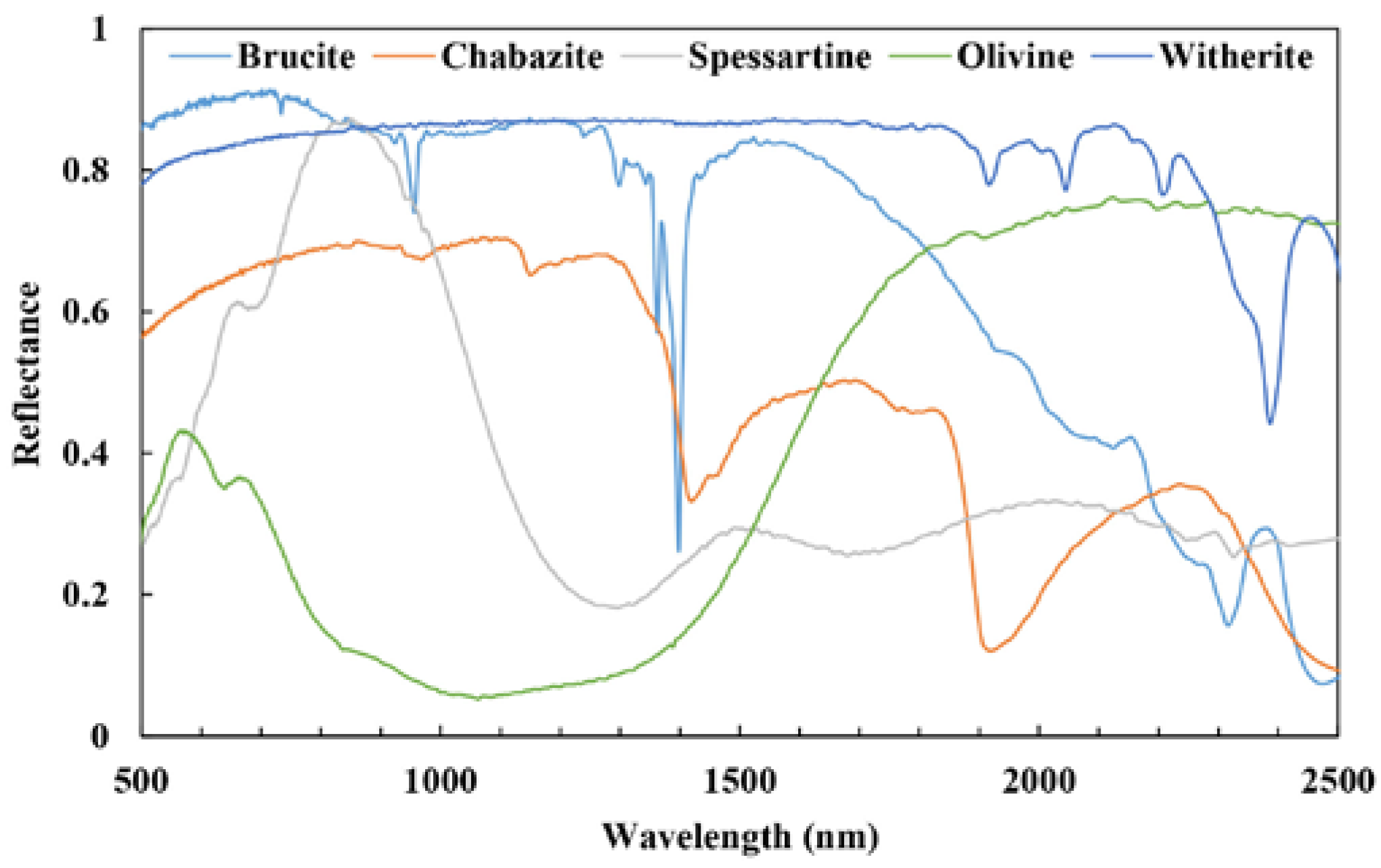
The hyperspectral synthetic data were generated using five spectral signatures randomly selected from the United States Geological Survey (USGS) digital spectral library [54], i.e., those for brucite, chabazite, olivine, spessartine and witherite (Figure 2). These spectral signatures are linearly independent and can be regarded as endmembers [16]. All signatures are available online (http://speclab.cr.usgs.gov/spectral-lib.html). The spectral data contain 420 bands covering wavelengths from 395.1–2560 nm. To create the linear mixtures, the abundance of each endmember was randomly determined using the Dirichlet distribution under the ANC and ASC. Moreover, to simulate possible errors and sensor noise, zero mean white Gaussian noise with a 30-dB signal-to-noise ratio (SNR), as defined in [55], was added to the mixture dataset.

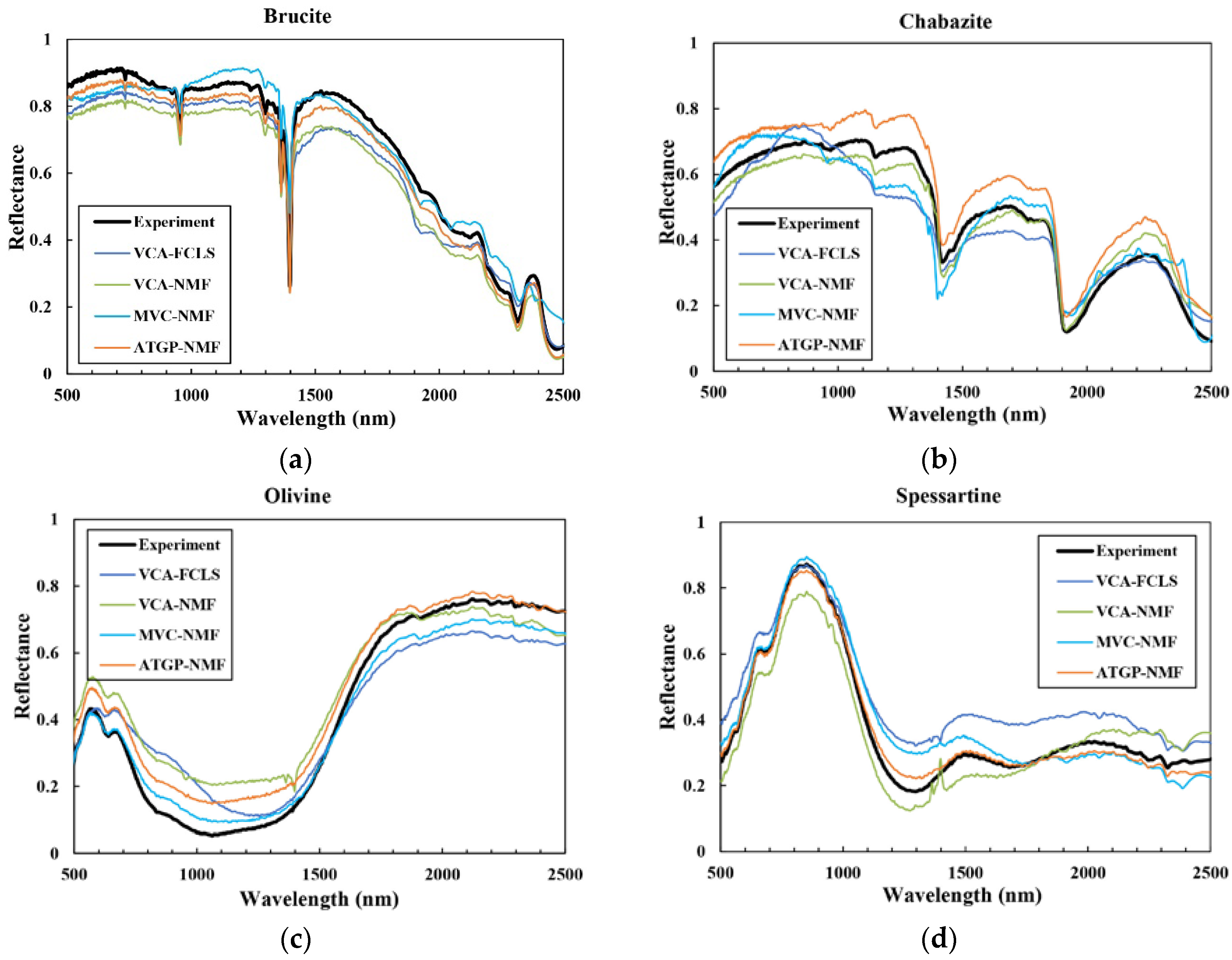
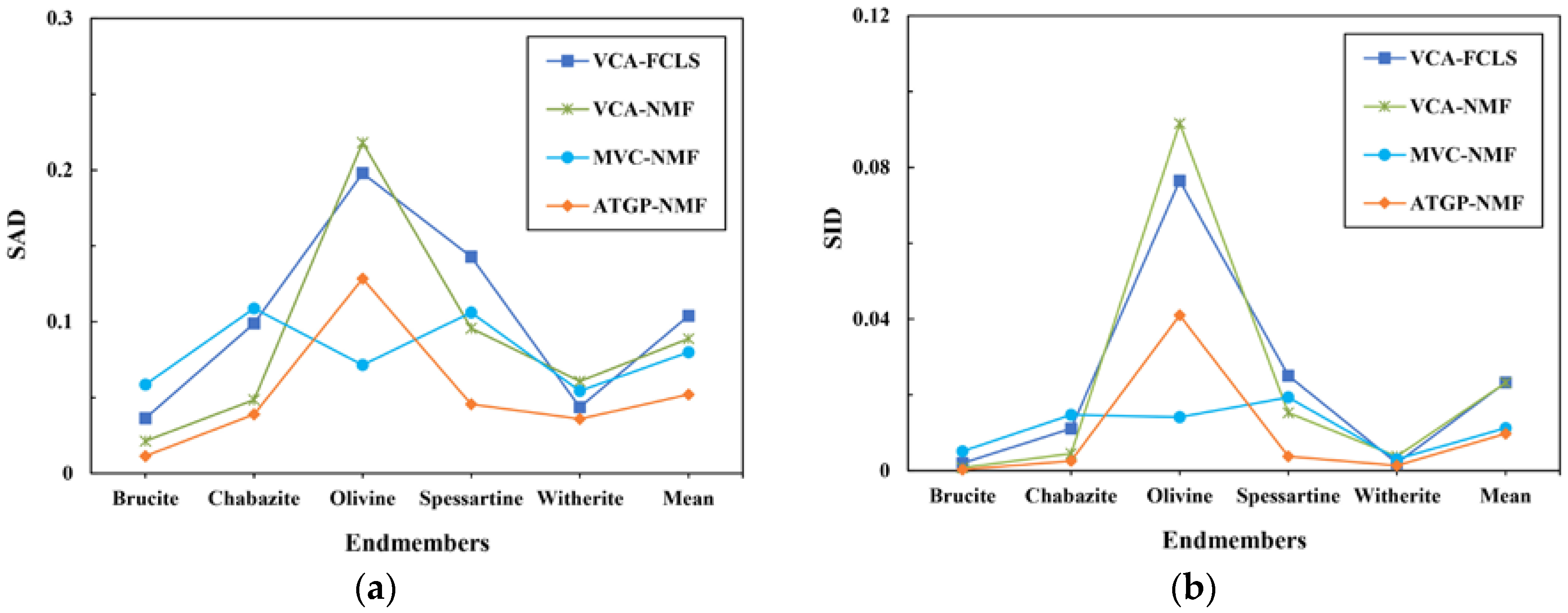
The abovementioned four algorithms, including the ATGP-NMF, VCA-NMF, MVC-NMF and VCA-FCLS algorithms, were first applied to the synthetic mixture data (SNR = 30 dB, purity level ρ = 0.8) to extract the endmember spectra (Figure 3) and calculate the corresponding abundances. The similarity of the extracted spectra to the real spectra was evaluated by SAD and SID (Figure 4). The accuracy of the abundance estimation was evaluated by RMSE (

Table 1. Spectral angle distance (SAD), spectral information divergence (SID) and RMSE values of the four algorithms on synthetic data.

Method	SAD	SID	RMSE
VCA-FCLS	0.1039	0.0233	0.1002
VCA-NMF	0.0888	0.0232	0.0867
MVC-NMF	0.0798	0.0113	0.0576
ATGP-NMF	0.0520	0.0098	0.0549

).

As shown in Figure 3 and Figure 4, the spectra extracted by the proposed ATGP-NMF algorithm are quite similar to the real spectra, with smooth curves and little noise, followed by those extracted by the MVC-NMF, VCA-NMF and VCA-FCLS algorithms. In this experiment, although a pure pixel does not exist (purity level ρ = 0.8), the purity level of the synthetic mixture data is higher. Therefore, the endmember spectra extracted by VCA-FCLS also resemble the real endmember spectra, with small SAD and SID values.

To further evaluate the robustness of these four algorithms, we compared their performances under different conditions, in terms of the SNR, purity level ρ and number of endmembers p, by using synthetic data. The comparison results are shown in Figure 5, Figure 6 and Figure 7.

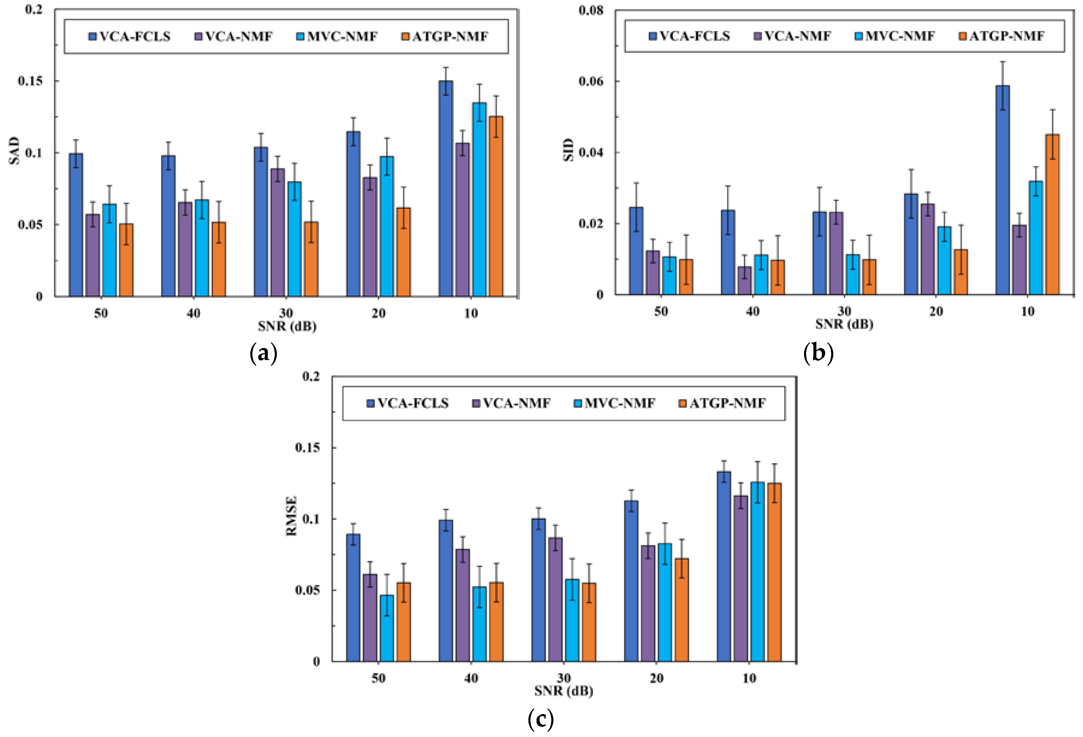
(1) Robustness to noise interference: In this experiment, tests of the algorithms’ sensitivities to noise were carried out by changing the SNR level from 50 to 10 dB. The synthetic data consist of five endmembers, i.e., the spectral signatures selected from the USGS spectral library, at the purity level of 0.8, which means pure pixels do not exist. The SAD, SID and RMSE values of the four algorithms are shown in Figure 5a–c, respectively. The ATGP-NMF algorithm performed well, yielding lower SAD and SID values than the other algorithms at different SNR levels. With the decrease in SNR, the RMSE values of ATGP-NMF decreased and stabilized; for MVC-NMF, the RMSE values kept increasing.

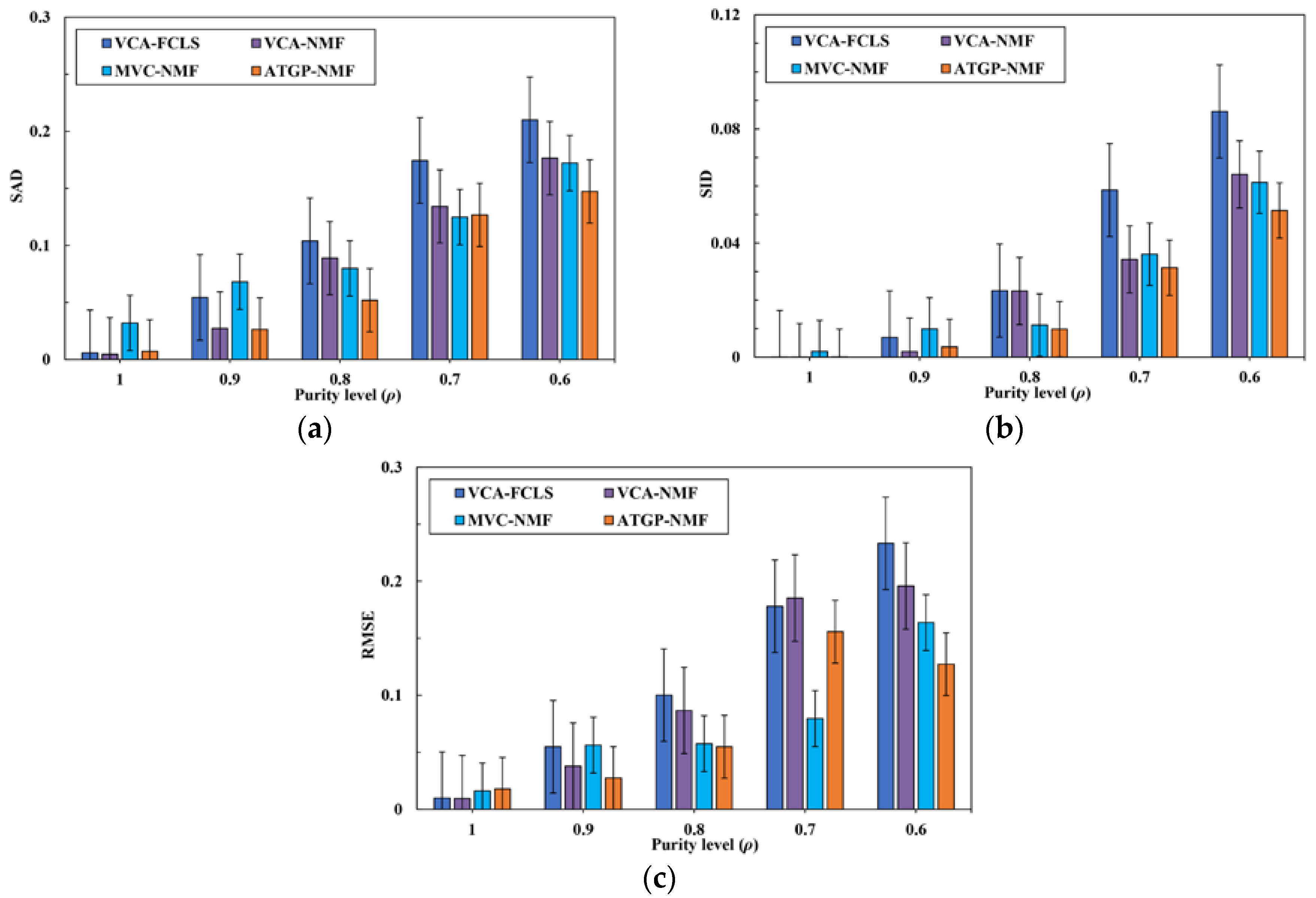
(2) Robustness to mixing degree: Following the method used in [56], we generated mixed spectra at different purity levels. In this experiment, we changed the purity level ρ from 1 to 0.6 with an SNR of 30 dB. The comparisons of the SAD, SID and RMSE values derived from the four algorithms are shown in Figure 6a–c. The SAD, SID and RMSE values of these four algorithms are inversely proportional to the purity level. At the purity level of one, i.e., when pure pixels exist, the algorithms of four methods all produced good solutions, with low SAD, SID and RMSE values. With regard to the purity level, the RMSE values of ATGP-NMF were lower overall than those of the other algorithms.

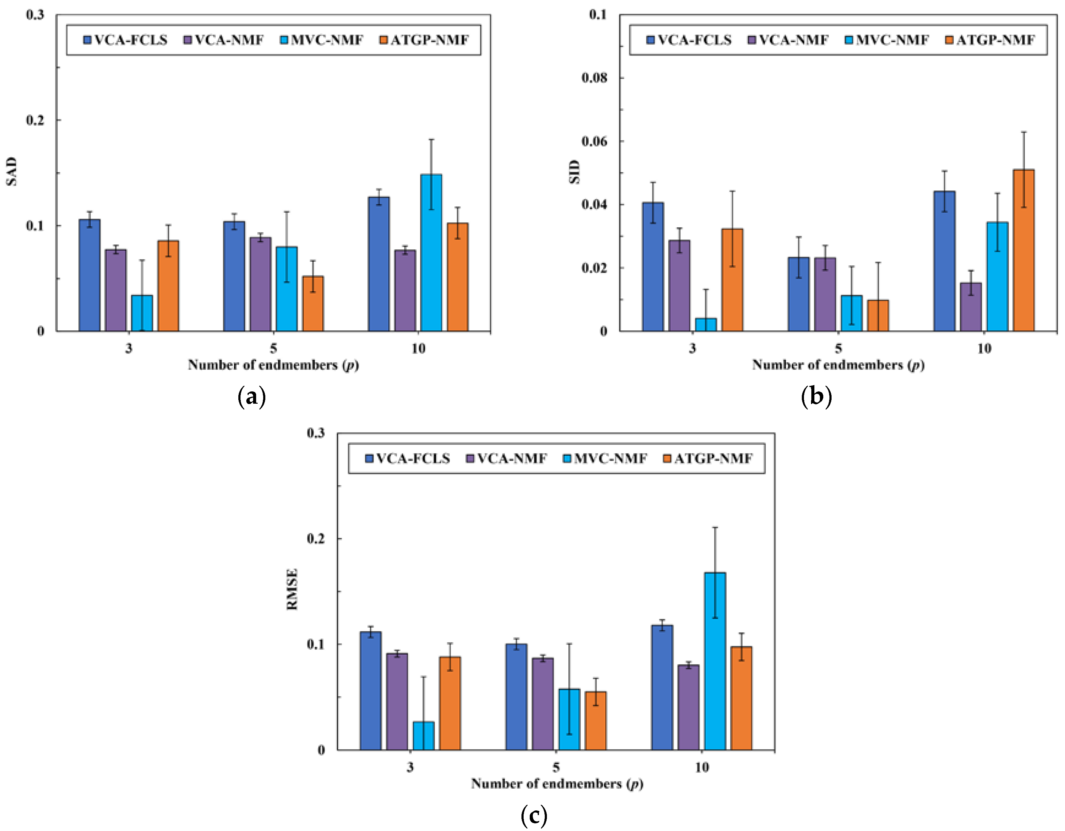
(3) Generalization of the number of endmembers: In this experiment, we generated mixed spectra with different numbers of endmembers to test these algorithms. The endmember numbers were set to 3, 5 and 10, while the SNR was set to 30 dB and the purity level was set to 0.8. When the number of endmembers was set to three, the mixed spectra were generated using the spectral signatures of brucite, chabazite and olivine. When the number of endmembers was set to 10, another five spectral signatures were selected from the USGS digital spectral library, in addition to the previously-selected five signatures. Figure 7a–c shows that the performances of VCA-NMF and ATGP-NMF are relatively better and more robust than those of the other algorithms for the tested number of endmembers.

3.3. Spectral Unmixing Using Berlin HyMap Image

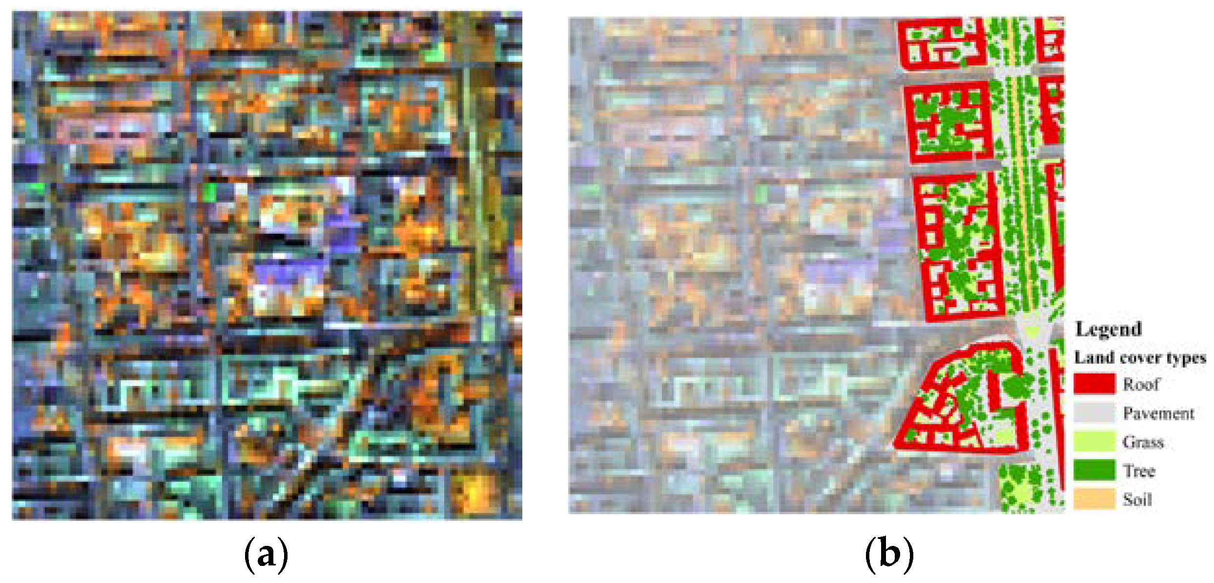
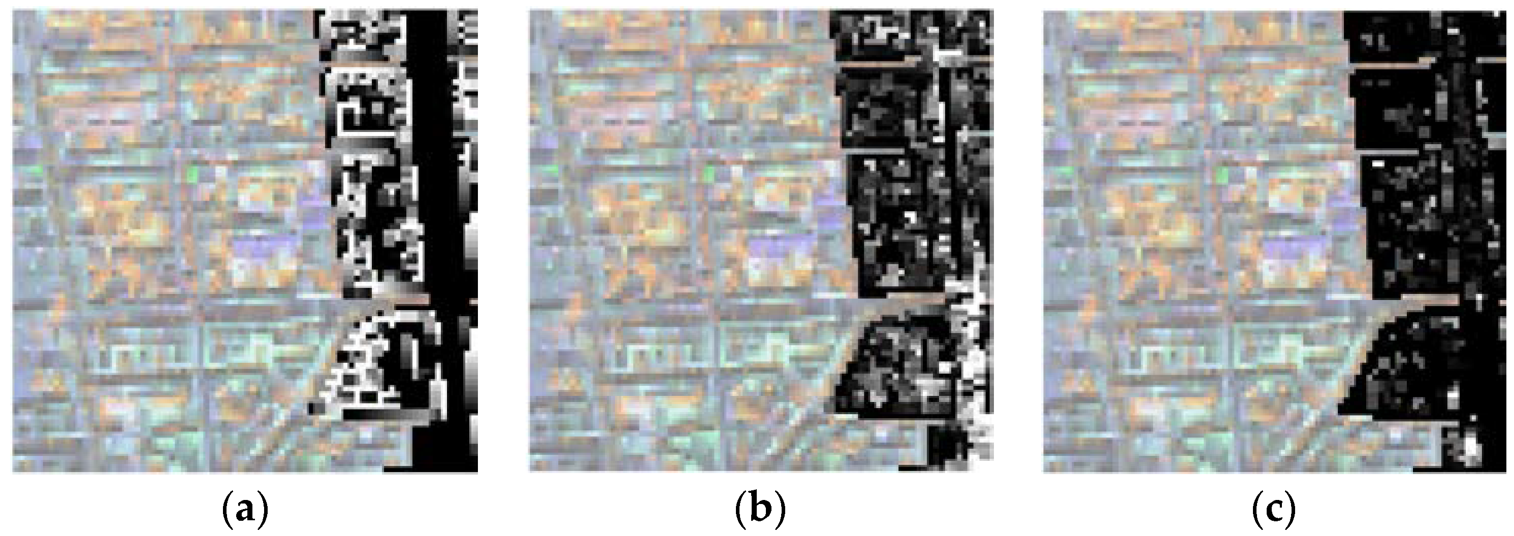
To evaluate the performance of the proposed ATGP-NMF algorithm on the real image, we conducted experiments on a subset of the Berlin-Urban-Gradient dataset, which mainly comprises a HyMap reflectance image, a library of material spectra and the reference land cover information [57]. More information on this dataset can be found in [58,59,60]. For this work, a subset with 80 × 80 pixels of the Berlin HyMap image (Figure 8a), acquired on 20 August 2009 at 9 m spatial resolution, was selected as the study data. The image contains 111 bands after removing noisy bands with spectral sampling distances between 13 and 17 nm, and spectral coverage from 440 to 2500 nm. Based on the reference land cover information, we considered five urban land cover types in the study area, i.e., roof, pavement, grass, tree and soil. The reference abundances of each land cover type (Figure 9), defined as the corresponding proportions at each pixel, were calculated based on the reference land cover map (Figure 8b). We selected the pixels with an area percentage of one and calculated their average spectral values as the reference spectrum of the land cover type. Because there were no pure pixels of the grass category, four pixels with an area percentage greater than 0.7 were selected instead.

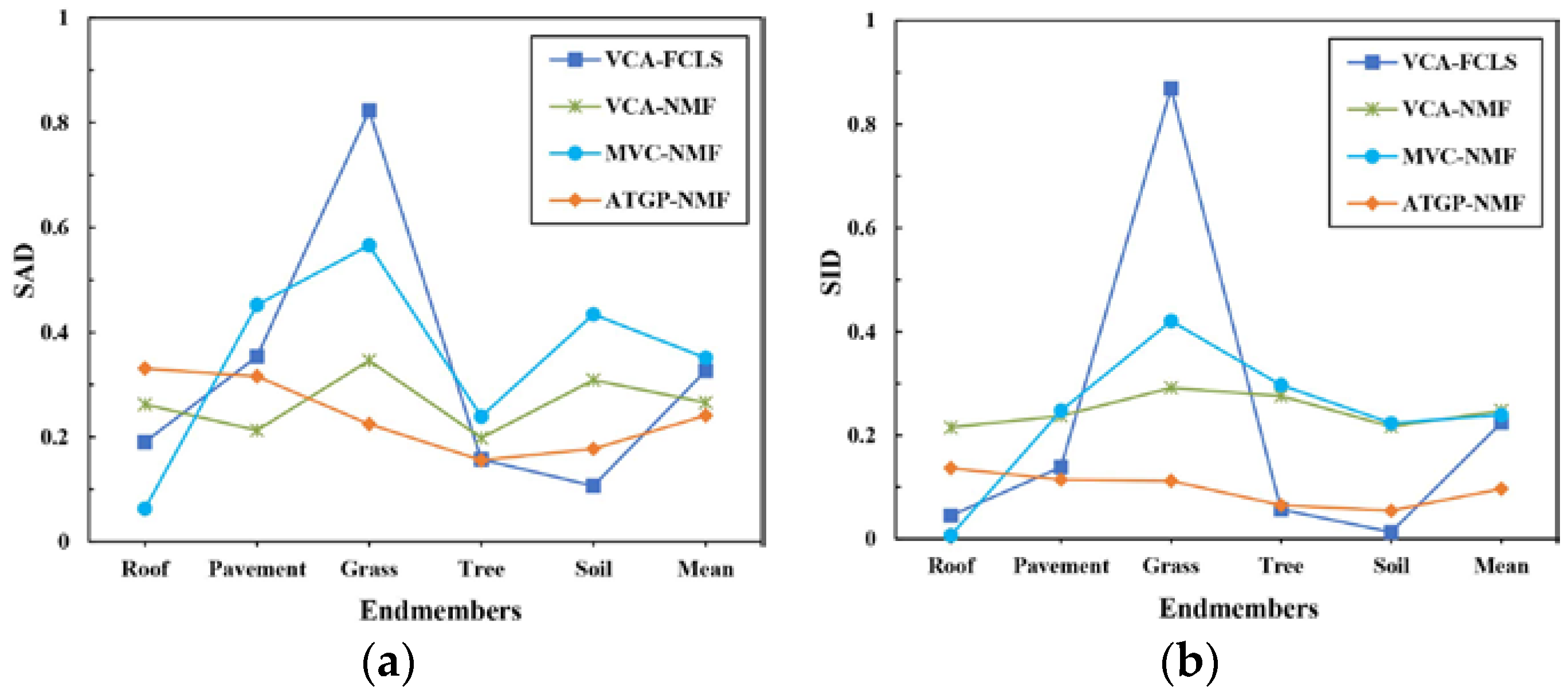
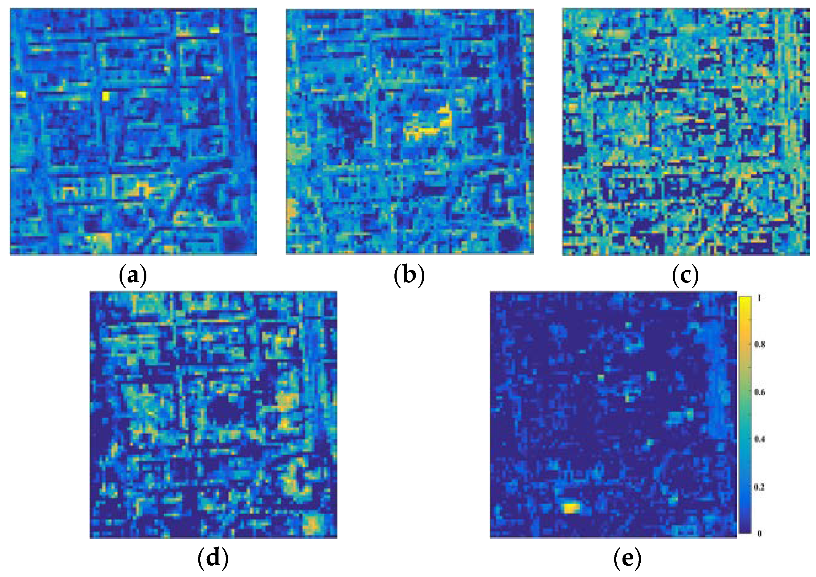
The comparisons of the VCA-FCLS, VCA-NMF, MVC-NMF and ATGP-NMF algorithms on the Berlin HyMap image are shown in Figure 10 and

Table 2. SAD, SID and RMSE values of different algorithms with the Berlin HyMap image.

Method	SAD	SID	RMSE
VCA-FCLS	0.3260	0.2246	0.3309
VCA-NMF	0.2655	0.2473	0.3249
MVC-NMF	0.3508	0.2389	0.3591
ATGP-NMF	0.2407	0.0965	0.3011

. Figure 10a,b shows that the proposed ATGP-NMF algorithm provided five endmembers with relatively low SAD and SID values. Figure 11 shows the estimated abundance maps by ATGP-NMF. Comparing to the reference abundance maps (Figure 9), it is demonstrated that the ATGP-NMF algorithm can produce satisfactory abundance separation. For all four algorithms, the estimated spectra of grass are in bad accordance with the reference endmembers. In the study area, grasses are scattered mainly around the buildings and trees, which are susceptible to the shadows of the buildings and trees and the spectral similarity between the grasses and trees.

3.4. Spectral Unmixing Using a Hyperion Image

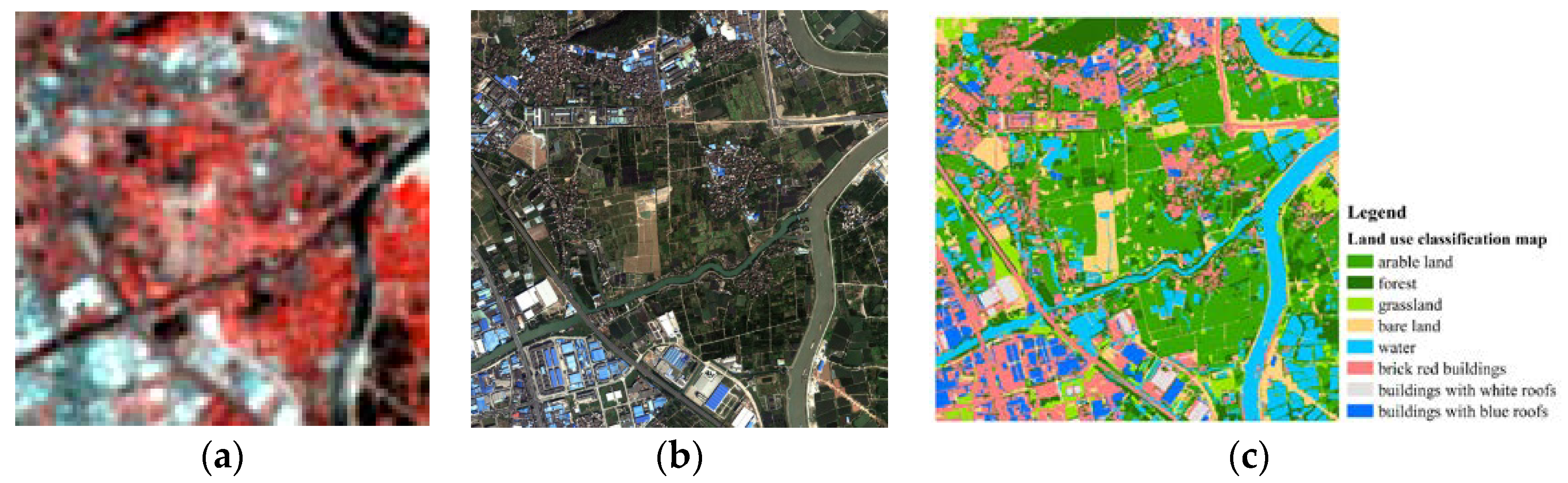
We used a Hyperion image to further verify the applicability of the proposed ATGP-NMF algorithm in complicated situations. The Hyperion image (Figure 12a), acquired on 19 January 2011, covers parts of Guangzhou and Foshan, both of which are cities in Guangdong Province, China. The test image of this study is a subset of 101 × 101 pixels with 30-m spatial resolution. In addition, the image contains 242 bands acquired in the spectral range of 356–2577 nm. To improve the spectral unmixing performance, a series of pretreatments was performed on this image, including radiometric calibration and atmospheric correction. In addition, we removed the low SNR bands and the water vapor absorption bands. A total of 158 bands (including Bands 8–57, 79–120, 133–165 and 188–220) were used in this experiment.

For the Hyperion image, the number of endmembers was estimated using HFC mentioned in Section 2.3. Considering the actual situation of the study area, we finally determined that there are eight endmembers in the study area. In this study, the reference abundances were extracted from a high-resolution remote sensing image acquired from Google Earth (Figure 12b). The classification map of the eight land cover types of the study area (Figure 12c) was then acquired through supervised classification of the high-resolution remote sensing image using the k-nearest neighbor [61]. Finally, the area percentage of each land cover type in one 30 × 30 m pixel was calculated and considered as its endmember abundance (Figure 13). In addition, due to the variability of the endmember spectra, we selected reference endmember spectra from the Hyperion image. We selected 30 samples for each land cover type and used the average spectra of these 30 samples as the reference spectra for each land cover type.

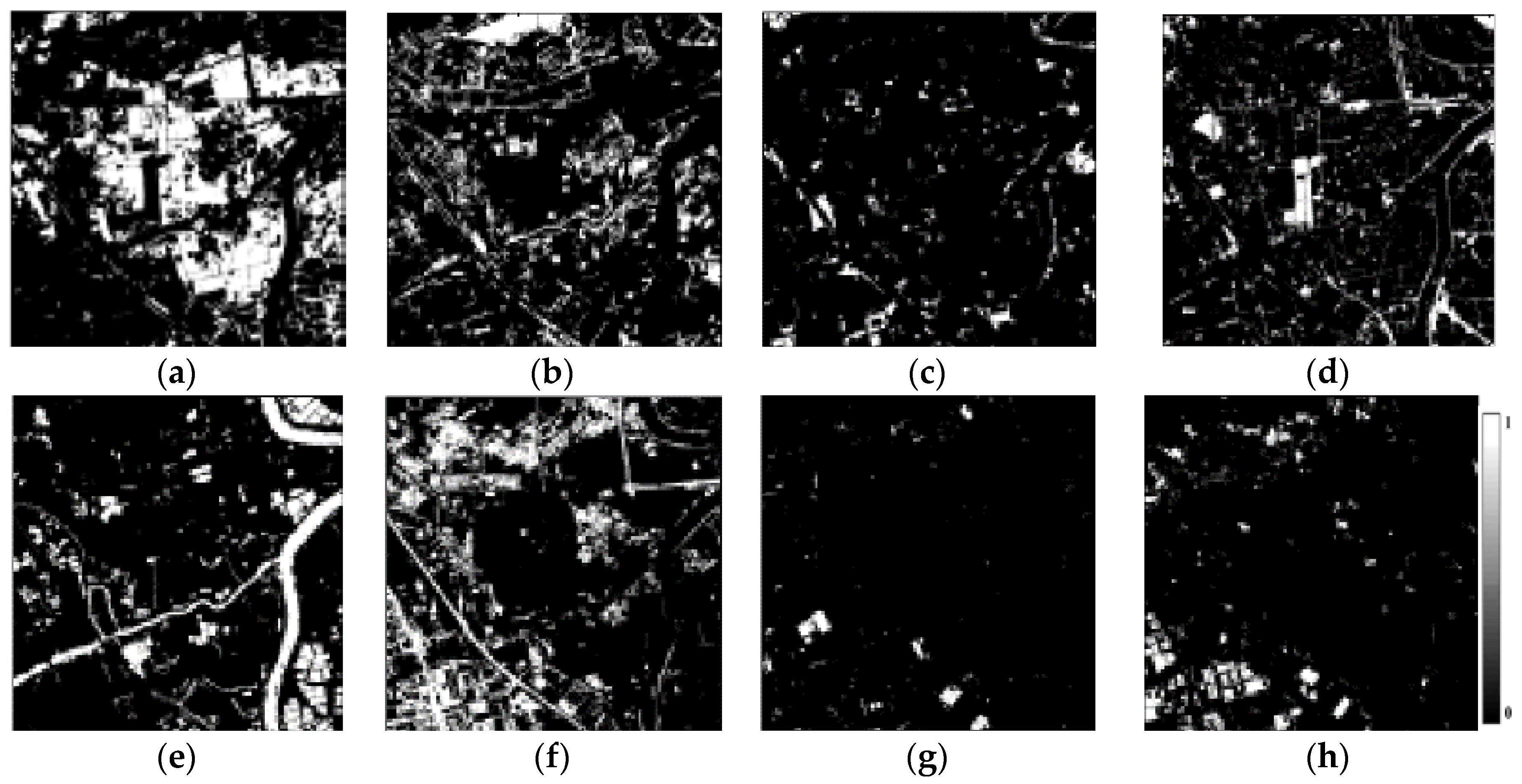
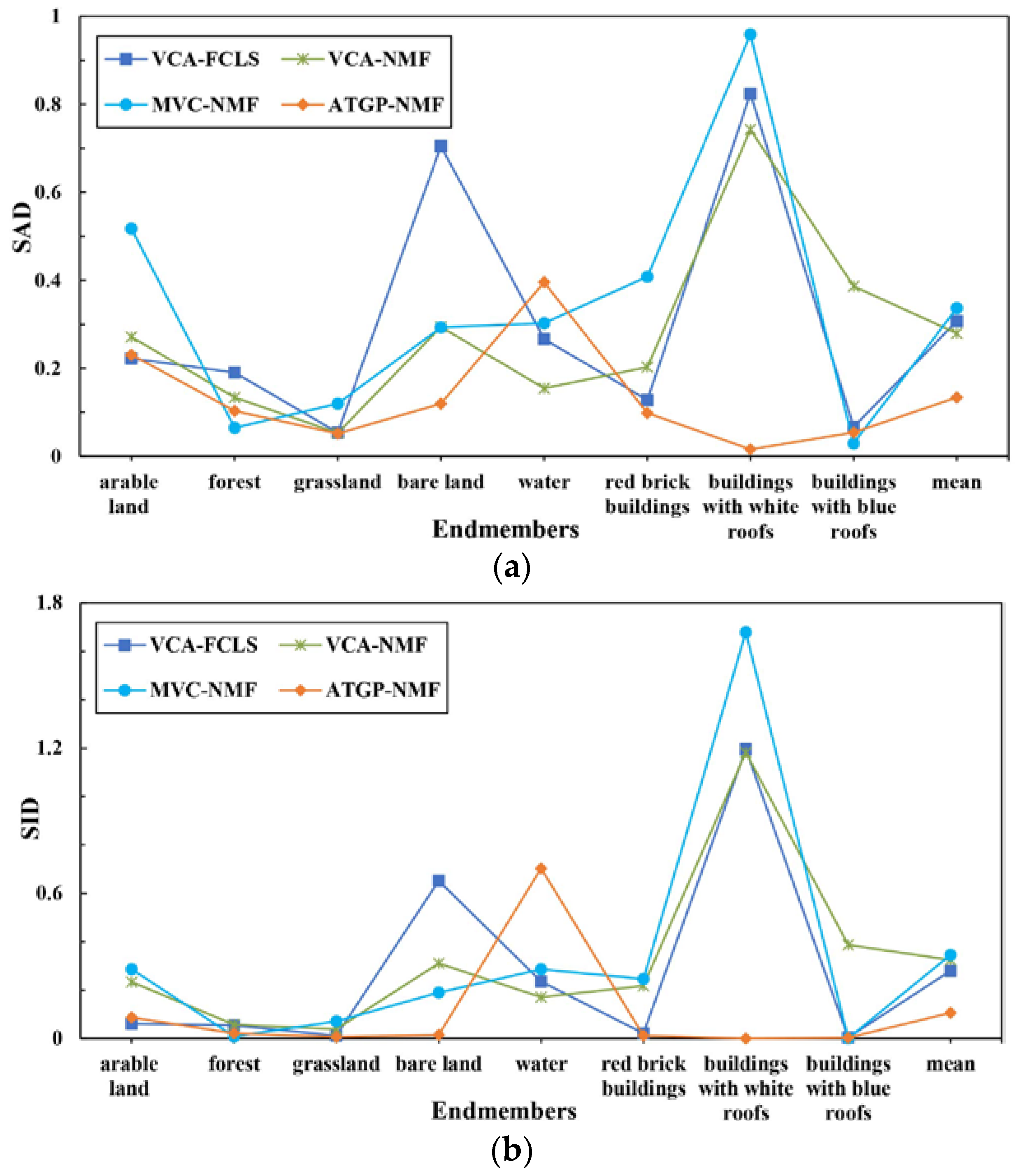
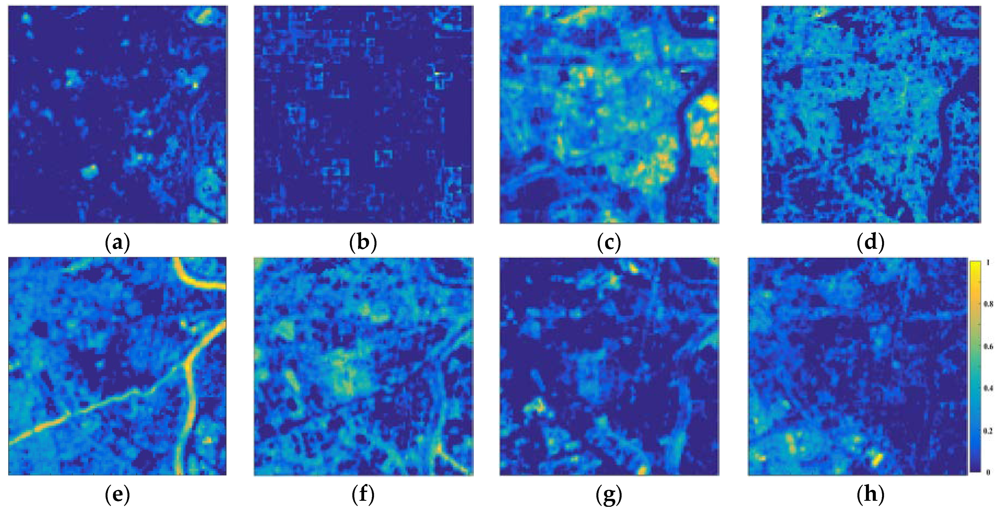
The comparison of the SAD and SID values of the four algorithms is shown in Figure 14, while the errors of the abundance estimation are given in

Table 3. SAD, SID and RMSE values of different algorithms with the Hyperion image.

Method	SAD	SID	RMSE
VCA-FCLS	0.3072	0.2797	0.3101
VCA-NMF	0.2798	0.3249	0.2866
MVC-NMF	0.3368	0.3459	0.2732
ATGP-NMF	0.1338	0.1061	0.2659

. As shown in Figure 14a,b, the proposed ATGP-NMF algorithm provided eight endmembers with relatively low SAD and SID values. Compared to those of the other three algorithms, the spectra extracted by ATGP-NMF are closer to those of the actual land cover types. The ATGP-NMF algorithm can extract endmembers with high correlations, such as buildings with white roofs and blue roofs. Figure 15 shows the abundance maps estimated by ATGP-NMF. The distribution of the estimated endmembers is close to the distribution of their corresponding land cover types. Table 3 shows that the ATGP-NMF algorithm yielded the most accurate abundance estimation results with the lowest RMSE for the hyperspectral image. This is primarily because the ATGP-NMF algorithm can effectively and efficiently find the most representative endmember spectra from hyperspectral images. Among the four different algorithms, the traditional VCA-FCLS algorithm had the poorest performance, which again proves the advantages of blind unmixing methods.

3.5. Computational Efficiency

To evaluate the computational efficiency of the particular algorithm, the computing time was often used as an important measure in many related studies [35]. The computational efficiency of an algorithm can be defined as a numerical function T(n): time versus the input size n. In this study, since the input data are the same, we used the average computing time (in seconds) of each algorithm’s application on synthetic data, the Berlin HyMap image, and Hyperion image to evaluate their computational efficiency. The four algorithms were executed in Mathworks MATLAB R2014b on a computer with Intel(R) Xeon(R) E3-1246 CPU (3.50 GHz) and 12 GB RAM. For the three NMF derivative algorithms, i.e., VCA-NMF, MVC-NMF and ATGP-NMF, the endmember spectral and abundance estimation results were determined at the maximum iteration number of 300.

Table 4. Computing time (seconds) of different methods on synthetic data, the Berlin HyMap image, and Hyperion Image.

Method	VCA-FCLS	VCA-NMF	MVC-NMF	ATGP-NMF
Synthetic Data	0.83	0.61	0.98	0.59
Berlin HyMap Image	2.15	1.99	65.26	1.95
Hyperion Image	9.37	4.37	165.66	5.28

shows that the computing time of the proposed ATGP-NMF algorithm is less than those of the traditional two-stage VCA-FCLS algorithm and the MVC-NMF algorithm. The MVC-NMF algorithm required more processing time than the other three algorithms, particularly for processing the real image. With the endmember initialization, the proposed ATGP-NMF and the existing VCA-NMF required less computation time. Table 4 also shows that ATGP-generated initial endmembers can significantly reduce the computational time of the spectral unmixing process. This is mainly because ATGP only needs to process previously-generated target pixels, not the whole dataset, to extract endmembers [42].

4. Conclusions

The traditional NMF algorithm suffers from the “local best” problem, which greatly limits its applications. In this paper, via the use of ATGP-generated initial target endmembers, the ATGP-NMF algorithm is proposed to improve the performance of NMF in hyperspectral unmixing. The ATGP algorithm is introduced to provide more accurate initial points to identify endmembers, which can then be used by the NMF to obtain the global solutions for hyperspectral unmixing. Furthermore, the proposed ATGP-NMF algorithm requires little prior knowledge and can be applied in complex situations, even if there are no pure pixels.

Experiments were carried out to evaluate the performances of ATGP-NMF and three other algorithms, namely, VCA-NMF, MVC-NMF, and VCA-FCLS, using synthetic hyperspectral data and real hyperspectral images. Based on analysis of the experimental results, the following conclusions can be made: (1) The traditional two-stage spectral unmixing method, VCA-FCLS, can only achieve satisfactory results when pure pixels exist. When there are little prior knowledge and no pure pixels, the studied BSS methods, namely, VCA-NMF and ATGP-NMF, and MVC-NMF without the pure pixel assumption can achieve better unmixing results than VCA-FCLS. (2) Of all the algorithms, the ATGP-NMF algorithm demonstrated the best applicability and consistently produced good results in different situations. The extracted endmember spectra were closer to the real spectra, and the abundance estimation was more accurate. (3) Proper endmember initialization can help the NMF algorithm yield better estimation results with less computation time.

References

- Goetz, A.F.H.; Vane, G.; Solomon, J.E.; Rock, B.N. Imaging spectrometry for earth remote sensing. Science 1985, 228, 1147–1153. [Google Scholar] [CrossRef] [PubMed]
- Heinz, D.C. Fully constrained least squares linear spectral mixture analysis method for material quantification in hyperspectral imagery. IEEE Trans. Geosci. Remote Sens. 2001, 39, 529–545. [Google Scholar] [CrossRef]
- Nascimento, J.M.; Dias, J.M. Vertex component analysis: A fast algorithm to unmix hyperspectral data. IEEE Trans. Geosci. Remote Sens. 2005, 43, 898–910. [Google Scholar] [CrossRef]
- Wei, Y.; Jin, C.; Peng, G. A new spectral mixture analysis method based on spectral correlation matching. J. Remote Sens. 2008, 12, 454–461. (In Chinese) [Google Scholar]
- Chen, J.; Jia, X.; Yang, W.; Matsushita, B. Generalization of subpixel analysis for hyperspectral data with flexibility in spectral similarity measures. IEEE Trans. Geosci. Remote Sens. 2009, 47, 2165–2171. [Google Scholar] [CrossRef] [Green Version]
- Li, X.; Wang, J.; Hu, B.; Strahler, A. Application of priori knowledge in remote sensing inversion. Sci. China (Ser. D) 1998, 28, 67–72. (In Chinese) [Google Scholar]
- Haykin, S.; Chen, Z. The cocktail party problem. Neural Comput. 2005, 17, 1875–1902. [Google Scholar] [CrossRef] [PubMed]
- Hyvärinen, A.; Oja, E. Independent component analysis: Algorithms and applications. Neural Netw. 2000, 13, 411–430. [Google Scholar] [CrossRef]
- Lee, D.D.; Seung, H.S. Learning the parts of objects by non-negative matrix factorization. Nature 1999, 401, 788–791. [Google Scholar] [CrossRef] [PubMed]
- Jia, S.; Qian, Y. Spectral and spatial complexity-based hyperspectral unmixing. IEEE Trans. Geosci. Remote Sens. 2007, 45, 3867–3879. [Google Scholar] [CrossRef]
- Georgiev, P.; Theis, F.; Cichocki, A. Sparse component analysis and blind source separation of underdetermined mixtures. IEEE Trans. Neural Netw. 2005, 16, 992–996. [Google Scholar] [CrossRef] [PubMed]
- Zhong, Y.; Wang, X.; Zhao, L.; Feng, R.; Zhang, L.; Xu, Y. Blind spectral unmixing based on sparse component analysis for hyperspectral remote sensing imagery. ISPRS-J. Photogramm. Remote Sens. 2016, 119, 49–63. [Google Scholar] [CrossRef]
- Cai, D.; He, X.; Han, J.; Huang, T.S. Graph regularized nonnegative matrix factorization for data representation. IEEE Trans. Pattern Anal. Mach. Intell. 2011, 33, 1548–1560. [Google Scholar] [CrossRef] [PubMed]
- Pauca, V.P.; Piper, J.; Plemmons, R.J. Nonnegative matrix factorization for spectral data analysis. Linear Algebra Its Appl. 2006, 416, 29–47. [Google Scholar] [CrossRef]
- Pascual-Montano, A.; Carazo, J.M.; Kochi, K.; Lehmann, D.; Pascual-Marqui, R.D. Nonsmooth nonnegative matrix factorization (nsNMF). IEEE Trans. Pattern Anal. Mach. Intell. 2006, 28, 403–415. [Google Scholar] [CrossRef] [PubMed]
- Miao, L.; Qi, H. Endmember extraction from highly mixed data using minimum volume constrained nonnegative matrix factorization. IEEE Trans. Geosci. Remote Sens. 2007, 45, 765–777. [Google Scholar] [CrossRef]
- Li, E.; Zou, Y.; Su, B. Research of the sparseness constraint MVC-NMF algorithm. Hydrogr. Surv. Charting 2011, 31, 43–46. (In Chinese) [Google Scholar]
- Yang, Z.; Zhou, G.; Xie, S.; Ding, S.; Yang, J.; Zhang, J. Blind spectral unmixing based on sparse nonnegative matrix factorization. IEEE Trans. Image Process. 2011, 20, 1112–1125. [Google Scholar] [CrossRef] [PubMed]
- Bioucas-Dias, J.M.; Plaza, A.; Dobigeon, N.; Parente, M.; Du, Q.; Gader, P.; Chanussot, J. Hyperspectral unmixing overview: Geometrical, statistical, and sparse regression-based approaches. IEEE J. Sel. Top. Appl. Earth Observ. Remote Sens. 2012, 5, 354–379. [Google Scholar] [CrossRef]
- Ma, W.K.; Bioucas-Dias, J.M.; Chan, T.H.; Gillis, N.; Gader, P.; Plaza, A.J.; Ambikapathi, A.; Chi, C.Y. A signal processing perspective on hyperspectral unmixing: Insights from remote sensing. IEEE Signal Process. Mag. 2014, 31, 67–81. [Google Scholar] [CrossRef]
- Kizel, F.; Shoshany, M.; Netanyahu, N.S.; Even-Tzur, G.; Benediktsson, J.A. A stepwise analytical projected gradient descent search for hyperspectral unmixing and its code vectorization. IEEE Trans. Geosci. Remote Sens. 2017, 55, 4925–4943. [Google Scholar] [CrossRef]
- Yokoya, N.; Yairi, T.; Iwasaki, A. Coupled nonnegative matrix factorization unmixing for hyperspectral and multispectral data fusion. IEEE Trans. Geosci. Remote Sens. 2012, 50, 528–537. [Google Scholar] [CrossRef]
- Yuan, Y.; Fu, M.; Lu, X. Substance dependence constrained sparse NMF for hyperspectral unmixing. IEEE Trans. Geosci. Remote Sens. 2015, 53, 2975–2986. [Google Scholar] [CrossRef]
- He, W.; Zhang, H.; Zhang, L. Total variation regularized reweighted sparse nonnegative matrix factorization for hyperspectral unmixing. IEEE Trans. Geosci. Remote Sens. 2017, 55, 3909–3921. [Google Scholar] [CrossRef]
- Tsinos, C.G.; Rontogiannis, A.A.; Berberidis, K. Distributed blind hyperspectral unmixing via joint sparsity and low-rank constrained non-negative matrix factorization. IEEE Trans. Comput. Imaging 2017, 3, 160–174. [Google Scholar] [CrossRef]
- Wang, W.; Qian, Y. Adaptive L1/2 sparsity-constrained NMF with half-thresholding algorithm for hyperspectral unmixing. IEEE J. Sel. Top. Appl. Earth Observ. Remote Sens. 2015, 8, 2618–2631. [Google Scholar] [CrossRef]
- He, W.; Zhang, H.; Zhang, L. Sparsity-regularized robust non-negative matrix factorization for hyperspectral unmixing. IEEE J. Sel. Top. Appl. Earth Observ. Remote Sens. 2016, 9, 4267–4279. [Google Scholar] [CrossRef]
- Salehani, Y.E.; Gazor, S. Smooth and sparse regularization for NMF hyperspectral unmixing. IEEE J. Sel. Top. Appl. Earth Observ. Remote Sens. 2017, 10, 3677–3692. [Google Scholar] [CrossRef]
- Li, J.; Bioucas-Dias, J.M.; Plaza, A.; Liu, L. Robust collaborative nonnegative matrix factorization for hyperspectral unmixing. IEEE Trans. Geosci. Remote Sens. 2016, 54, 6076–6090. [Google Scholar] [CrossRef]
- Wang, R.; Li, H.; Liao, W.; Huang, X. Endmember initialization method for hyperspectral data unmixing. J. Appl. Remote Sens. 2016, 10, 042009. [Google Scholar] [CrossRef]
- Liu, Z.; Tan, V.Y.F. Rank-one NMF-based initialization for NMF and relative error bounds under a geometric assumption. IEEE Trans. Signal Process. 2017, 65, 4717–4731. [Google Scholar] [CrossRef]
- Boutsidis, C.; Gallopoulos, E. Svd based initialization: A head start for nonnegative matrix factorization. Pattern Recognit. 2008, 41, 1350–1362. [Google Scholar] [CrossRef]
- Xue, Y.; Tong, C.S.; Chen, Y.; Chen, W.S. Clustering-based initialization for non-negative matrix factorization. Appl. Math. Comput. 2008, 205, 525–536. [Google Scholar] [CrossRef]
- Tang, A.W.; Shi, Z.; An, Z. Nonnegative matrix factorization for hyperspectral unmixing using prior knowledge of spectral signatures. Opt. Eng. 2012, 51, 087001. [Google Scholar] [CrossRef]
- Chang, C.I.; Li, Y. Recursive band processing of automatic target generation process for finding unsupervised targets in hyperspectral imagery. IEEE Trans. Geosci. Remote Sens. 2016, 54, 5081–5094. [Google Scholar] [CrossRef]
- Chang, C.I.; Plaza, A. A fast iterative algorithm for implementation of pixel purity index. IEEE Geosci. Remote Sens. Lett. 2006, 3, 63–67. [Google Scholar] [CrossRef]
- Yao, S.; Zeng, W.; Wang, N.; Chen, L. Validating the performance of one-time decomposition for fMRI analysis using ICA with automatic target generation process. Magn. Reson. Imaging 2013, 31, 970–975. [Google Scholar] [CrossRef] [PubMed]
- Keshava, N. A survey of spectral unmixing algorithms. Lincoln Lab. J. 2003, 14, 55–78. [Google Scholar]
- Xu, X.; Shi, Z. Multi-objective based spectral unmixing for hyperspectral images. ISPRS-J. Photogramm. Remote Sens. 2017, 124, 54–69. [Google Scholar] [CrossRef]
- Lee, D.D.; Seung, H.S. Algorithms for non-negative matrix factorization. In Advances in Neural Information Processing Systems; MIT Press: Cambridge, MA, USA, 2001; pp. 556–562. [Google Scholar]
- Tao, X. Research of Spectral Unmixing Based on Linear Model for Multi-Channel Remote Sensing Images. Master’s Thesis, Fudan University, Shanghai, China, 2008. (In Chinese). [Google Scholar]
- Plaza, A.; Chang, C.I. Impact of initialization on design of endmember extraction algorithms. IEEE Trans. Geosci. Remote Sens. 2006, 44, 3397–3407. [Google Scholar] [CrossRef]
- Ren, H.; Chang, C.I. Automatic spectral target recognition in hyperspectral imagery. IEEE Trans. Aerosp. Electron. Syst. 2006, 39, 1232–1249. [Google Scholar] [CrossRef]
- Harsanyi, J.C.; Farrand, W.H.; Chang, C.I. Determining the number and identity of spectral endmembers: An integrated approach using neyman-pearson eigen-thresholding and iterative constrained rms error minimization. In Proceedings of the 9th Thematic Conference on Geologic Remote Sensing, Pasadena, CA, USA, 8–11 February 1993. [Google Scholar]
- Du, Q.; Raksuntorn, N.; Younan, N.H.; King, R.L. End-member extraction for hyperspectral image analysis. Appl. Opt. 2008, 47, 77–84. [Google Scholar] [CrossRef]
- Pan, B.; Shi, Z.; Xu, X. R-vcanet: A new deep-learning-based hyperspectral image classification method. IEEE J. Sel. Top. Appl. Earth Observ. Remote Sens. 2017, 10, 1975–1986. [Google Scholar] [CrossRef]
- Chang, C.I.; Wen, C.H.; Wu, C.C. Relationship exploration among PPI, ATGP and VCA via theoretical analysis. Int. J. Comput. Sci. Eng. 2013, 8, 361–367. [Google Scholar] [CrossRef]
- Chang, C.I.; Chen, S.Y.; Li, H.C.; Chen, H.M.; Wen, C.H. Comparative study and analysis among ATGP, VCA, and SGA for finding endmembers in hyperspectral imagery. IEEE J. Sel. Top. Appl. Earth Observ. Remote Sens. 2016, 9, 4280–4306. [Google Scholar] [CrossRef]
- Merentitis, A.; Debes, C.; Heremans, R. Ensemble learning in hyperspectral image classification: Toward selecting a favorable bias-variance tradeoff. IEEE J. Sel. Top. Appl. Earth Observ. Remote Sens. 2014, 7, 1089–1102. [Google Scholar] [CrossRef]
- Liu, R.; Du, B.; Zhang, L. Hyperspectral unmixing via double abundance characteristics constraints based NMF. Remote Sens. 2016, 8, 464. [Google Scholar] [CrossRef]
- Mirzal, A. NMF versus ICA for blind source separation. Adv. Data Anal. Classif. 2017, 11, 25–48. [Google Scholar] [CrossRef]
- Pan, B.; Shi, Z.; Xu, X. Hierarchical guidance filtering-based ensemble classification for hyperspectral images. IEEE Trans. Geosci. Remote Sens. 2017, 55, 4177–4189. [Google Scholar] [CrossRef]
- Plaza, A.; Martinez, P.; Perez, R.; Plaza, J. A quantitative and comparative analysis of endmember extraction algorithms from hyperspectral data. IEEE Trans. Geosci. Remote Sens. 2004, 42, 650–663. [Google Scholar] [CrossRef]
- Clark, R.N.; Swayze, G.A.; King, T.V.V.; Gallagher, A.J.; Calvin, W.M. The US Geological Survey, Digital Spectral Reflectance Library: Version 1: 0.2 to 3.0 Microns; NASA: Washington, DC, USA, 1993. [Google Scholar]
- Harsanyi, J.C.; Chang, C.I. Hyperspectral image classification and dimensionality reduction: An orthogonal subspace projection approach. IEEE Trans. Geosci. Remote Sens. 1994, 32, 779–785. [Google Scholar] [CrossRef]
- Chan, T.H.; Chi, C.Y.; Huang, Y.M.; Ma, W.K. A convex analysis-based minimum-volume enclosing simplex algorithm for hyperspectral unmixing. IEEE Trans. Signal Process. 2009, 57, 4418–4432. [Google Scholar] [CrossRef]
- Okujeni, A.; Van Der Linden, S.; Hostert, P. Berlin-Urban-Gradient Dataset 2009-An EnMAP Preparatory Flight Campaign (Datasets). Available online: http://dataservices.gfz-potsdam.de/enmap/showshort.php? id=escidoc:1823890 (accessed on 17 April 2018).
- Okujeni, A.; van der Linden, S.; Hostert, P. Extending the vegetation–impervious–soil model using simulated enmap data and machine learning. Remote Sens. Environ. 2015, 158, 69–80. [Google Scholar] [CrossRef]
- Okujeni, A.; van der Linden, S.; Tits, L.; Somers, B.; Hostert, P. Support vector regression and synthetically mixed training data for quantifying urban land cover. Remote Sens. Environ. 2013, 137, 184–197. [Google Scholar] [CrossRef]
- Degerickx, J.; Okujeni, A.; Iordache, M.D.; Hermy, M.; van der Linden, S.; Somers, B. A novel spectral library pruning technique for spectral unmixing of urban land cover. Remote Sens. 2017, 9, 565. [Google Scholar] [CrossRef]
- Cover, T.; Hart, P. Nearest neighbor pattern classification. IEEE Trans. Inf. Theory 1967, 13, 21–27. [Google Scholar] [CrossRef]
Figure 1.
Flowchart of the proposed blind unmixing method improved by ATGP-generated initial target endmembers.
Figure 2.
Reflectance spectra of the five materials selected from the USGS spectral library.
Figure 3.
Comparison of the extracted endmember signatures using vertex component analysis (VCA)-fully-constrained least squares (FCLS), VCA-NMF, minimum volume constrained (MVC)-NMF and ATGP-NMF with the experiment data, spectral signals from the USGS digital spectral library for (a) brucite; (b) chabazite; (c) olivine; (d) spessartine; (e) witherite.
Figure 4.
(a) Spectral angle distance (SAD) and (b) spectral information divergence (SID) of different endmembers with the synthetic data determined using VCA-FCLS, VCA-NMF, MVC-NMF, and ATGP-NMF.
Figure 5.
Performance comparison at different noise levels (ρ = 0.8, p = 5) in terms of: (a) SAD; (b) SID; and (c) RMSE.
Figure 6.
Results of the algorithms with different purity levels (SNR = 30 dB, p = 5). (a) SAD; (b) SID; and (c) RMSE.
Figure 7.
Performance comparison at different numbers of endmembers (SNR = 30 dB, ρ = 0.8). (a) SAD; (b) SID; and (c) RMSE.
Figure 8.
(a) A subset of the Berlin HyMap image (R = 833 nm, G = 1652 nm, B = 632 nm); (b) the reference land cover map of the study area.
Figure 9.
Reference abundance maps of five land cover types: (a) roof; (b) pavement; (c) grass; (d) tree; (e) soil.
Figure 10.
SAD (a) and SID (b) of different endmembers with the Berlin HyMap image using VCA-FCLS, VCA-NMF, MVC-NMF, and ATGP-NMF.
Figure 11.
Abundance maps provided by ATGP-NMF with the Berlin HyMap image: (a) roof; (b) pavement; (c) grass; (d) tree; (e) soil.
Figure 12.
(a) Hyperion image of the study area (R = 936 nm, G = 2143 nm, B = 2345 nm); (b) the high-resolution remote sensing image covering the study area; (c) the land use classification map of the study area.
Figure 13.
Reference abundance maps of eight land cover types: (a) arable land; (b) forest; (c) grassland; (d) bare land; (e) water; (f) red brick buildings; (g) buildings with white roofs; (h) buildings with blue roofs.
Figure 14.
SAD (a) and SID (b) of different endmembers with the Hyperion image using VCA-FCLS, VCA-NMF, MVC-NMF and ATGP-NMF.
Figure 15.
Abundance maps provided by ATGP-NMF with the Hyperion image: (a) arable land; (b) forest; (c) grassland; (d) bare land; (e) water; (f) red brick buildings; (g) buildings with white roofs; (h) buildings with blue roofs.