An Automated Processing Method for Agglomeration Areas

1
Chinese Academy of Surveying and Mapping, Beijing 100830, China
2
College of Geomatics, Shandong University of Science and Technology, Qingdao 266590, China
*
Author to whom correspondence should be addressed.
ISPRS Int. J. Geo-Inf. 2018, 7(6), 204; https://doi.org/10.3390/ijgi7060204
Submission received: 11 April 2018
/
Revised: 7 May 2018
/
Accepted: 27 May 2018
/
Published: 29 May 2018
Abstract
:Agglomeration operations are a core component of the automated generalization of aggregated area groups. However, because geographical elements that possess agglomeration features are relatively scarce, the current literature has not given sufficient attention to agglomeration operations. Furthermore, most reports on the subject are limited to the general conceptual level. Consequently, current agglomeration methods are highly reliant on subjective determinations and cannot support intelligent computer processing. This paper proposes an automated processing method for agglomeration areas. Firstly, the proposed method automatically identifies agglomeration areas based on the width of the striped bridging area, distribution pattern index (DPI), shape similarity index (SSI), and overlap index (OI). Next, the progressive agglomeration operation is carried out, including the computation of the external boundary outlines and the extraction of agglomeration lines. The effectiveness and rationality of the proposed method has been validated by using actual census data of Chinese geographical conditions in the Jiangsu Province.
1. Introduction
Agglomeration is a geometric transformation in which the structural characteristics of aggregate area groups are retained. In this transformation, narrow and empty gaps (i.e., bridging areas) between regularly organized area groups are reduced to lines, which transforms areas that are segmented by bridging areas into agglomerated area elements. In the context of this paper, an area group is not a set of area elements with arbitrary structures or shapes as this term specifically refers to contiguous sets of areas, with similar shape features that are also organized in certain patterns and separated by striped bridging areas. When the scale of a map is being reduced, striped bridging areas inside aggregated area groups are difficult to represent on maps due to their long and narrow shape. However, practical applications generally require the preservation of these structural characteristics. Hence, generalization algorithms that do not consider the internal structure of contiguous area groups, such as aggregation [1,2] and amalgamation [3,4] algorithms, cannot be utilized for the agglomeration of area groups.
In 1987, Delucia and Black [5] proposed an agglomeration algorithm for digital map generalization and described its fundamental concepts and ideas for the implementation of this operation. Li [6] further refined the implemented concepts for this algorithm. Some studies have also used agglomeration algorithms to generalize hydrological elements, such as scattered lakes and aquaculture areas, with the stitching of polygon boundaries along a skeleton line (figuratively described as “pulling up a zipper”), which conveyed excellent results. Although these studies provide theoretical procedures and operational concepts for the agglomeration algorithm, in-depth implementation details are lacking. Furthermore, although these procedures can be performed by experienced cartographers, they cannot be used for intelligent machine processing. In addition, researchers have not focused sufficiently on this issue because only a few geographic elements possess agglomeration features. Consequently, detailed and comprehensive investigations on agglomeration operations are scarce in the current literature. Therefore, it is very meaningful to propose a method for the intelligent computer processing of agglomeration operations. In this paper, we explore the automated identification of agglomeration areas and carry out the agglomeration operation, progressively, for these areas.
The remainder of this paper is organized as follows: Section 2 analyzes related works and the major problems preventing the automated agglomeration of aggregated area groups; Section 3 presents the methodology for the automated processing of agglomeration areas, including the automated identification of agglomeration areas and progressive agglomeration operation; Section 4 demonstrates the experiments and analyzes the results obtained; and Section 5 describes the discussion and conclusions.
2. Related Works
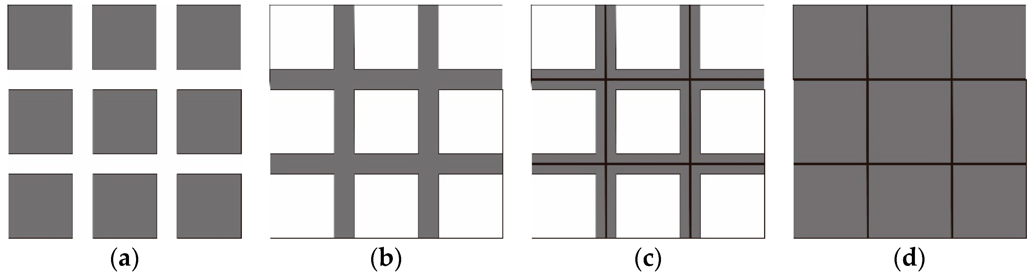
Li [6] introduces a basic idea regarding the implementation of agglomeration operations. Specifically, a minimum bounding rectangle (MBR) is used to supplement the original area group, and long and narrow bridging areas between the areas in the group are then extracted and transformed into operable elements. This step is followed by the extraction of skeletons for these bridging areas, which are used as new boundary lines for the area group, as shown in Figure 1.
Although a conceptual basis for the implementation of agglomeration algorithms is available in the literature, clearer and more specific operational details have yet to be provided on agglomeration algorithms, and some of the major problems preventing the automated agglomeration of aggregated area groups have yet to be solved. These major problems are outlined below.
Problem 1: In actual map databases, polygon elements with a variety of shapes are often distributed in an irregular manner within certain geographic regions. The identification of organized aggregated area groups (as shown in Figure 1a) is an important prerequisite for the realization of agglomeration operations. However, all reports in the current literature simply assume that agglomeration areas have been identified correctly, and agglomeration may simply be completed based on this hypothesis. Therefore, there is a lack of studies on the automated identification of agglomeration areas.
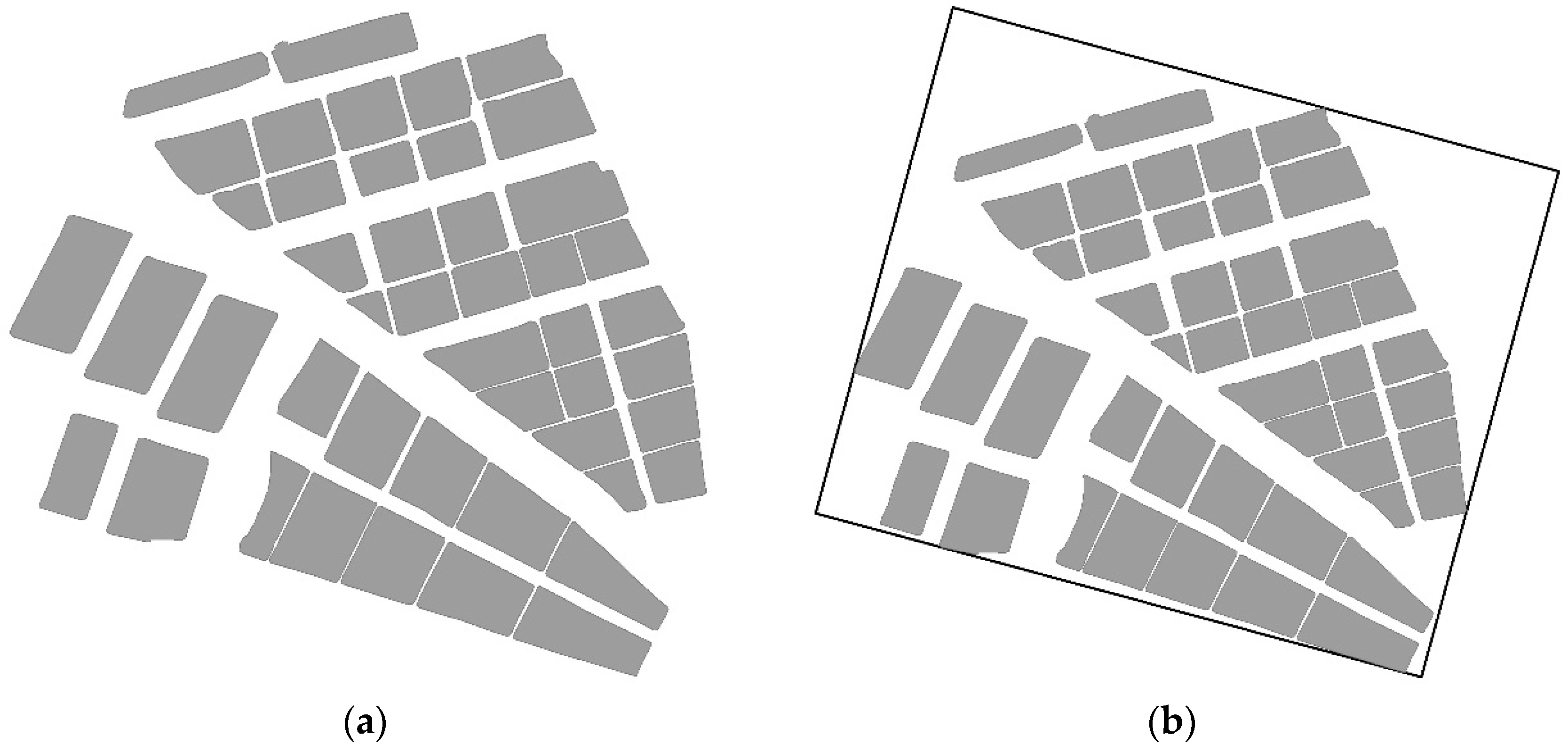
Problem 2: The external outlines of actual land objects are often irregular and may exhibit both concave and convex structures. Hence, the use of a convex hull, MBR, or minimum area-bounding rectangle (MABR) [7] to encompass these boundaries leads to redundant boundary spaces, as shown in Figure 2. In this scenario, the supplementation of original polygons during agglomeration results in a correct supplementation area that is exceeded and errors that are introduced during the skeleton extraction.
Problem 3: Delaunay triangulation is often used for the extraction of skeletons from map patches, as it possesses a number of highly desirable traits, such as adjacency, optimality, regional character, and convex polygons [8,9,10,11]. However, when a constrained Delaunay triangulation is used to extract the skeletons of junctions, the resulting skeletons exhibit jitters that do not accurately represent the primary shape of these bridging areas.
Problem 4: Because agglomeration is a map generalization operation, its effectiveness is dependent on the scale range of the map. The identification of a scale range is necessary for reducing the dimensionality of long and narrow bridging areas. However, the current literature has yet to consider the effects of scale range on agglomeration operations.
3. Methodology for the Automated Processing of Agglomeration Areas
3.1. Framework for the Proposed Method
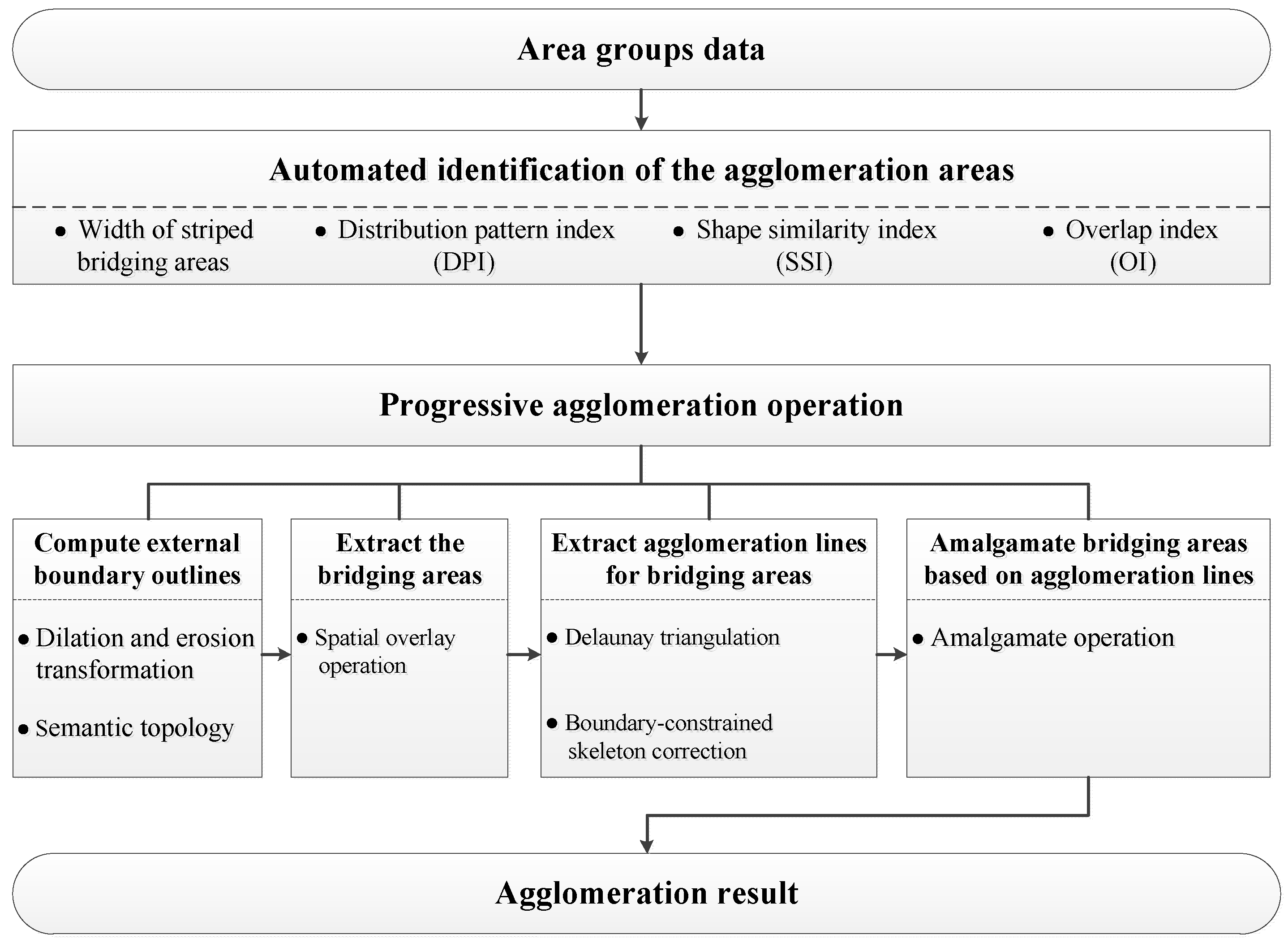
As depicted in Figure 3, our proposed method for the automated processing of agglomeration areas is composed of two parts: Identifying the agglomeration areas and performing the progressive agglomeration operation. The former is a prerequisite for the proposed method and the latter includes the key steps to implement this method.
Agglomeration areas are identified automatically based on four typical characteristics: Width of striped bridging areas, distribution pattern index (DPI), shape similarity index (SSI), and overlap index (OI).
Progressive agglomeration operations are carried out iteratively to handle the elements in agglomeration areas and they include four basic steps:
- (1)
- Computing the external boundary outlines for each agglomeration area;
- (2)
- Extracting bridging areas through the spatial overlay operation;
- (3)
- Extracting skeletons for bridging areas on the basis of the Delaunay triangulation and using the boundaries as constraints to correct the skeletons and form agglomeration lines; and
- (4)
- Amalgamating bridging areas based on agglomeration lines to obtain the agglomeration result.
The progressive agglomeration operation is a dynamic and iterative process. More details for this operation are presented in Section 3.3.
3.2. Automated Identification of Agglomeration Areas
Agglomeration involves the matching and connecting of similarly shaped area group elements that exhibit regular and aggregated distributions. However, in actual map databases, the shapes of aggregated area group elements tend to be highly complex and diverse, and have heterogeneous bridging area widths. Therefore, to perform an agglomeration operation, it is necessary to identify the regions containing area elements that satisfy the conditions for agglomeration (i.e., agglomeration areas).
3.2.1. Typical Characteristics of Agglomeration Areas
Width of Striped Bridging Area
Aggregated area groups present a variety of shapes. The width of a striped bridging area corresponds to the interval distance between adjacent area elements (TBDistance). If a map with an original scale of 1: Oscale is generalized to a target scale of 1: Tscale (Tscale > Oscale), the first task is to identify the striped bridging areas using a width threshold (BWthreshold) to determine whether an aggregated area group is an agglomeration area. The minimum visible distance on a conventional map may be calculated according to the target scale using Equation (1):
The census data of Chinese geographical conditions are used as an example and have an original scale of 1:10,000. The width thresholds, generalized to the target scale that is greater than 1:500,000 and smaller than 1:10,000, are shown in Table 1, in accordance with the technical specifications [12].
Based on the standard widths defined in Table 1, a map width of 0.4 mm was chosen as the threshold for the identification of striped bridging areas. Hence, Equation (1) may be simplified into Equation (2), which is in meters:
The width of the area element is equal to the distance between the area elements. Considering that the area shape influences the distance, Delaunay triangulation for the bridging areas is used to calculate the shape area. The calculation steps are as follows:
Firstly, the MBR is used to compute the boundaries of the aggregated area groups, as shown in Figure 4.
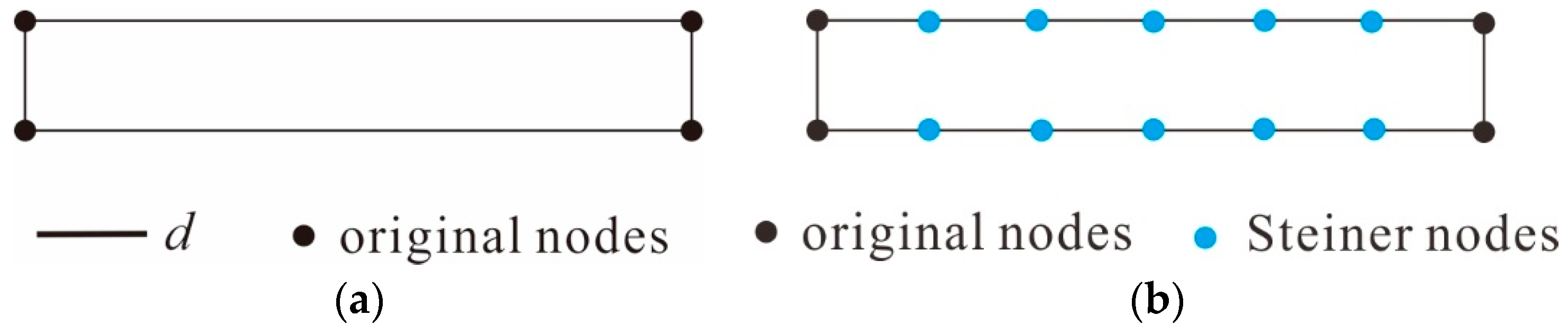
Secondly, Steiner nodes are added around the boundary of the MBR and each area element [13] because the original nodes are often used to describe the important morphological characteristics of an area feature (e.g., inflection nodes and intersection nodes). However, because there are usually only a few of these nodes, the triangles are stretched towards these points when constructing the triangulation. Because this Delaunay triangulation consists of more nodes and, thus, more triangles, the resulting skeleton is expected to be smoother. The specifics of this procedure are as follows: Firstly, a densification step, d, is defined, where d usually represents the length of the shortest arc segment in the boundary of an element. Sampling is then performed between two original nodes in intervals equal to d to obtain the Steiner points, as shown in Figure 5.
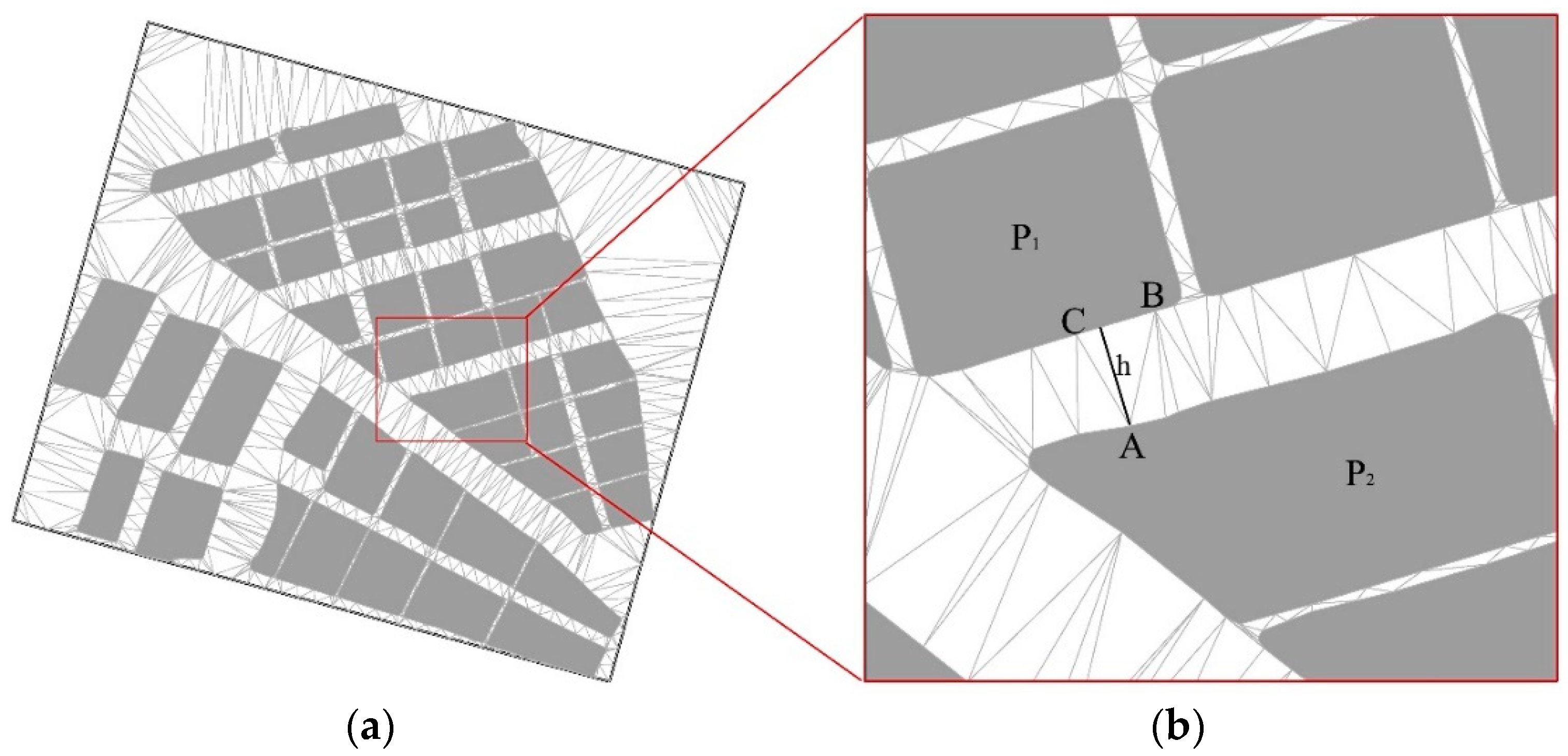
Thirdly, a boundary-constrained Delaunay triangulation is performed using a point-by-point insertion algorithm, as shown in Figure 6a.
The triangles in the constrained Delaunay triangulation connect area elements that are adjacent to each other, as shown in Figure 6b. In the figure, the adjacency between P1 and P2 is easily obtained from the edges of the triangle ABC (AB or AC). The heights (h) of all Delaunay triangles (i.e., the heights corresponding to the edges of the element boundary contours) between two adjacent area elements are then calculated, and the average height is taken as the distance between the adjacent elements (BDistance), as shown in Equation (3):
where n represents the total number of Delaunay triangles between two adjacent area elements.
Finally, if BDistance between two adjacent area elements is less than or equal to TBDistance (the threshold value for the widths of the bridging areas), these areas are then identified as candidates for agglomeration area subsets. The entirety of the candidate agglomeration area is extracted in this manner.
Distribution Pattern Index (DPI) of Area Elements
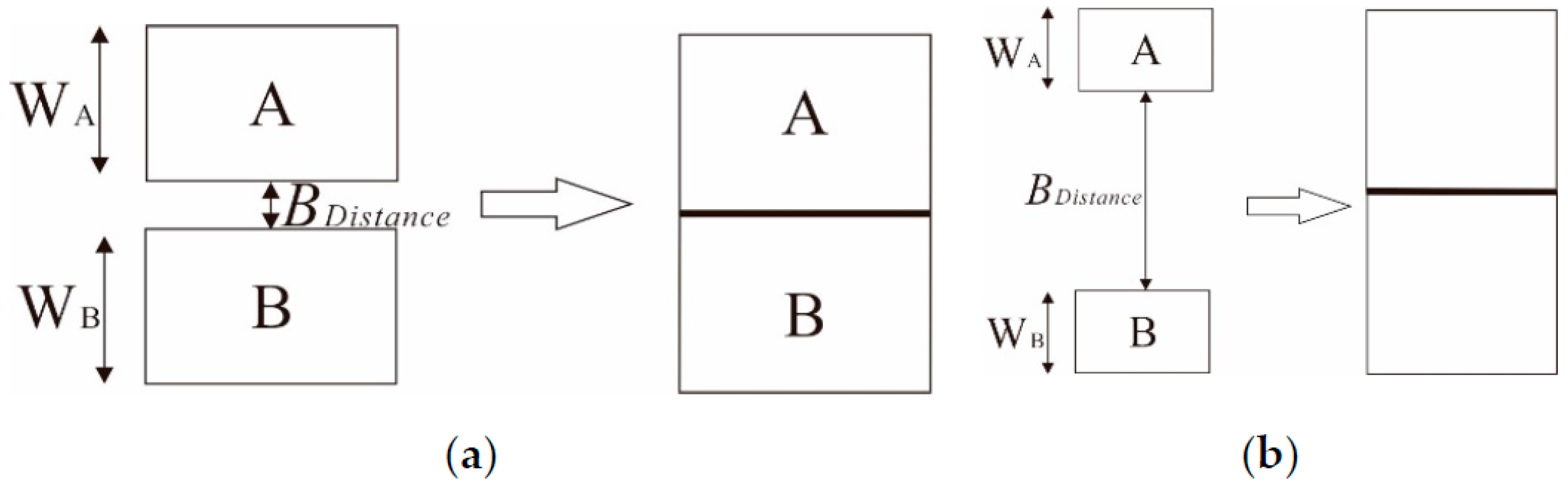
The relationship between the width of adjacent elements and the distance between adjacent elements reflects the internal structure of an aggregated area group from another perspective. When the sum of the widths for two adjacent area elements is larger than the width of the bridging area between them, an agglomeration operation clearly highlights the aggregation status of the area group without altering its spatial distribution characteristics. It is then appropriate to perform agglomeration on elements of this type, as shown in Figure 7a. When the sum of the width of two adjacent area elements is smaller than the width of the bridging area between them, large deformations occur after the agglomeration of these elements, which are, thus, unsuitable for agglomeration, as shown in Figure 7b.
Mitropoulos et al. [14] proposed a method for calculating the width of irregular areas (i.e., the average width, W), as defined in Equation (4):
where W represents the approximate average width of the elements, S represents the area of the patch, and BL represents the longest baseline of the patch (i.e., the length of the longest skeleton line in an area element), as shown by the bold line in Figure 8.
The W of an area element and BDistance can be used to construct the DPI, which gauges the spatial main-body degree of two area elements and their adjacency. This index is also used to determine whether two adjacent area elements should be agglomerated. represents the distribution pattern formed by two adjacent area elements, Xs and Xt, as shown in Equation (5):
where and represent the widths of and , respectively, and represents the distance between and .
The value of is proportional to the strength of the aggregation properties for the two adjacent area elements. Under normal circumstances, the threshold for agglomeration is = 1. It is, therefore, appropriate to perform an agglomeration operation only when ≥ 1.
Shape Similarity Index (SSI) of Area Elements
Because point-to-point distances and line segment angles are the two key elements in the line matching method proposed by Gabay and Doytsher [15], line segment angles are used to calculate the shape similarity between area elements in this paper. Firstly, to remove minute jitters in the boundaries, while retaining the main angles of the element, the Douglas-Peucker algorithm [16] was used to simplify the arc segments of each area element. In the next step, starting from the bottom-left corner of the area element, the angle of each arc segment is calculated sequentially in a counterclockwise direction. Angles greater than or equal to 45° reflect the primary shape of the element and are recorded. The consistency of the angles (in terms of size and order) in the two elements is then used to calculate their SSI values, as shown in Equation (6):
where and are internal angle sets for two adjacent area elements ( and , respectively) and represents the shape similarity between and .
Finally, the calculated SSI is compared with the threshold value to determine whether an agglomeration operation should be performed on the two area elements. In general, the angle threshold is 10°; thus, agglomeration is appropriate only if ≤ 10°.
Overlap Index (OI) of the Area Elements
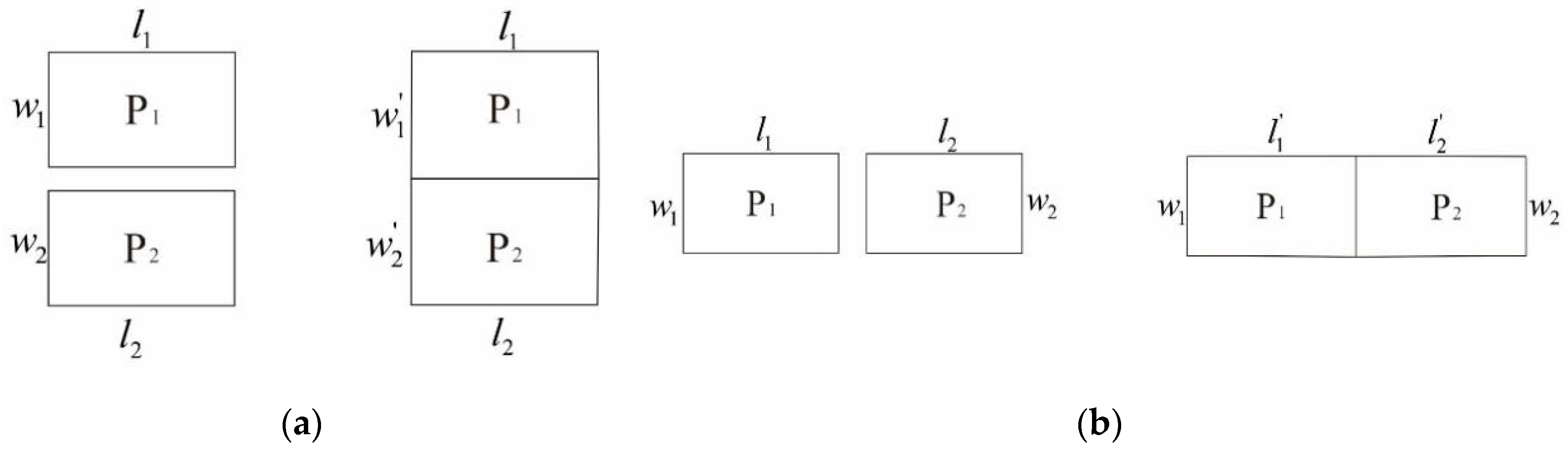
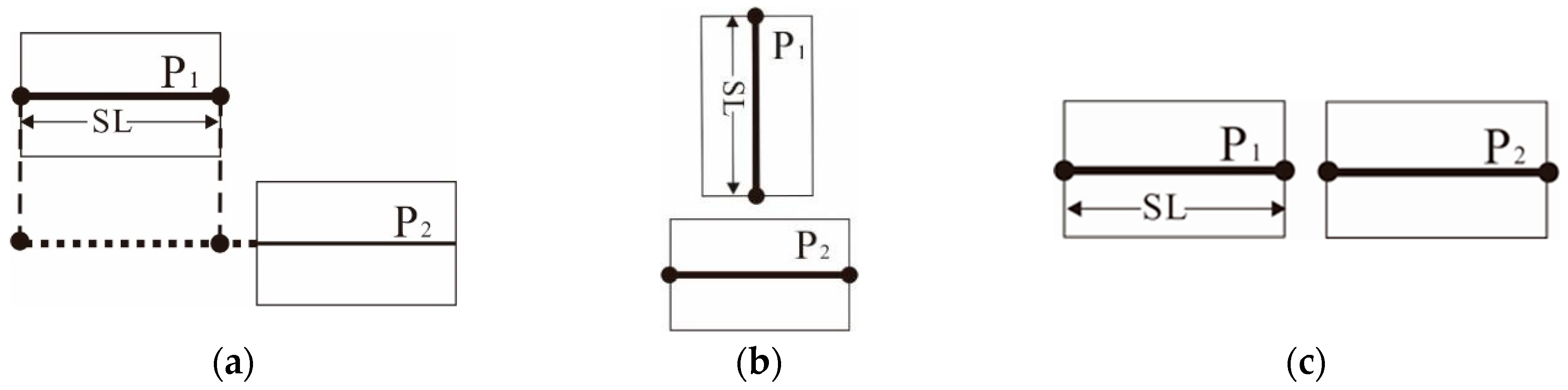
The longer edge of an area element is more representative of an element’s primary structure and extensional direction than its shorter edge. Hence, if two elements are side-adjacent to each other along their longer edges, these elements are then suitable for agglomeration, as shown in Figure 9a. Conversely, if the elements are side-adjacent along their shorter edges, the agglomeration of these elements is then inappropriate, as shown in Figure 9b.
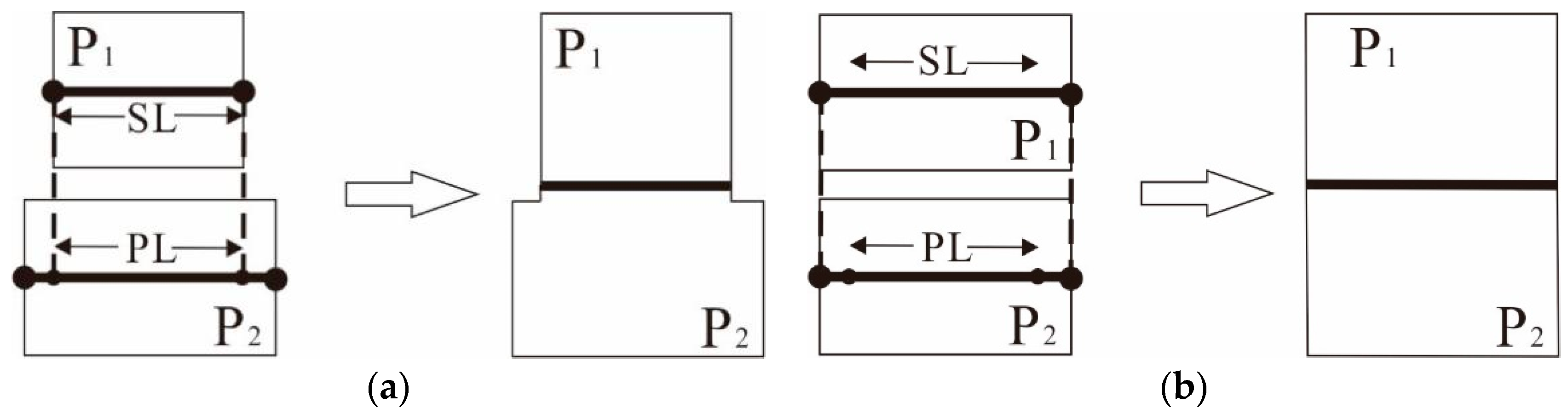
Using long edges that are projected onto each other, the long edges of each adjacent area element are replaced by the main skeleton during the process of calculation [17,18]. The ratio between the projection length (PL) and skeleton length (SL) is used to determine the OI of each element, as shown in Equation (7):
where and represent the overlap degrees of relative to and , and relative to , respectively. represents the PL obtained by projecting the main skeleton of onto the main skeleton of . represents the PL obtained by projecting the main skeleton of onto the main skeleton of . and represent the main SLs of and , respectively.
The value of OI ranges between 0 and 1, where a higher OI value indicates a higher degree of overlap between the two elements and a greater suitability for agglomeration, as shown in Figure 10a. When OI = 1, PL = SL, the elements are completely side-adjacent along their longer edges, as depicted in Figure 10b. When OI = 0, PL = 0, the elements are in a special state of side-adjacency, as shown in Figure 11. In general, the threshold for agglomeration is 0.5. If OI ≥ 0.5, agglomeration is deemed appropriate; otherwise, it is not inappropriate.
3.2.2. Identification
Given a set of area elements within some regions, , the suitability of an arbitrary pair of adjacent area elements for agglomeration can be determined in succession, according to the four structural characteristics described above. The subset of candidate agglomeration areas is determined by the width threshold of the striped bridging areas; for some arbitrary element, Pi, the elements that are suitable for agglomeration are then identified according to their DPI, SSI, and OI values to form the agglomeration area subset, Si.
Supposing that the agglomeration subsets of Pi, Pk, and Pm are , , and , respectively, in this case the computation of one of the agglomeration areas, , is shown in Equation (8):
All agglomeration area sets () are formed by repeating this process for all elements within the set of candidate agglomeration areas. The identification of agglomeration areas is, thus, completed in this manner. Agglomeration operations are then performed on each of these agglomeration areas.
3.3. Progressive Agglomeration Operation
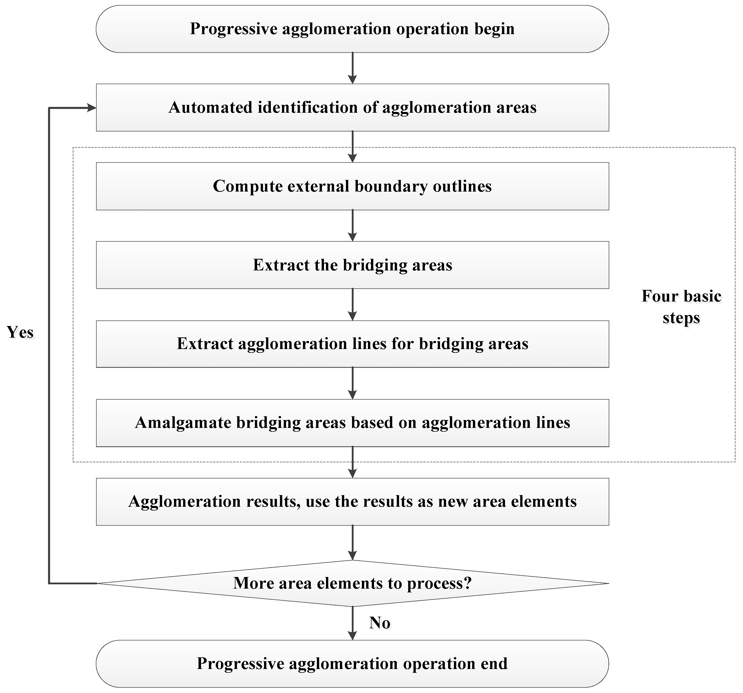
Because the automated identification of agglomeration areas is a dynamic and iterative process, a progressive agglomeration algorithm is proposed in this paper. An agglomeration operation is performed for each agglomeration area, which are identified by the aforementioned process in Section 3.2. The operation includes four basic steps: Computation of external boundary outlines, extraction of the bridging areas, extraction and correction of the bridging area agglomeration lines, and amalgamation of the bridging areas based on their agglomeration lines. Then, the first-stage agglomeration results can be obtained after the first operation, which forms new area groups. The new area groups are continuously identified by using the typical characteristics of agglomeration areas and are processed through agglomeration operations. These processes are repeated until all area elements are agglomerated. The entire workflow of the progressive agglomeration operation is illustrated in Figure 12.
As for the four basic steps in the progressive agglomeration operation, the extraction of bridging areas through the spatial overlay operation and the amalgamation of bridging areas based on skeletons are generally basic knowledge in the cartography field; therefore, they are not demonstrated in this paper. This study focuses on computing external boundary outlines, extracting agglomeration lines accurately, and performing the progressive process for the agglomeration operation; these processes are covered in more detail later in this paper.
3.3.1. Computation of External Boundary Outlines
The computation of external boundary outlines for an agglomeration area is the basis of the agglomeration algorithm. Furthermore, the accuracy of this computation has a direct impact on the subsequent extraction of bridging areas and bridging area skeletons. Therefore, the external boundary outlines must accurately describe the structural details (e.g., protrusion and concave characteristics) of the agglomeration area. However, there are significant deficiencies in the current methods in terms of their ability to preserve the structural features of boundaries (as shown in Figure 2b). To overcome these deficiencies, buffer zone transformations and semantic topologies are incorporated as constraints for the computation of external boundary outlines in this paper.
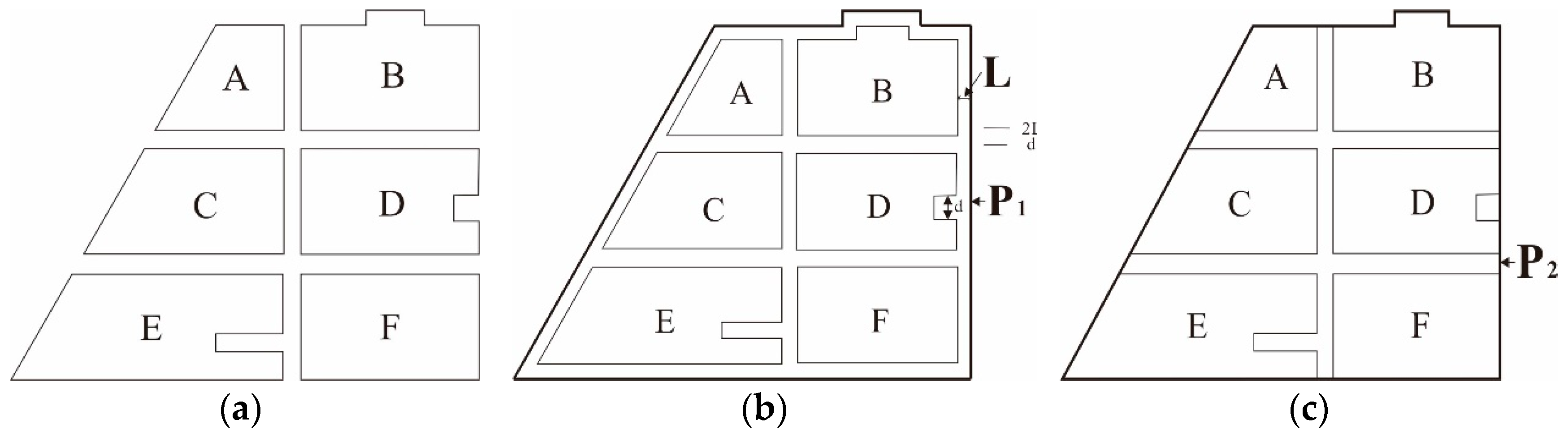
A dilation-erosion transformation for agglomeration areas, which is a morphological dilation [19] with a distance of L, is first performed on the original polygonal area group in the outward direction. After dilation, the overlapping parts of each polygon are then fused to obtain the boundary polygon, P1, as shown in Figure 13b. A morphological erosion with a distance, L, is then performed on P1 in the inward direction, which returns the P2 polygon, as shown in Figure 13c.
This transformation maintains convex and flat boundary areas, but smooths concave areas. The general shape of the figures remain unchanged because the protrusions and straight-line portions are unchanged. However, the concave areas in the polygon are fused with the remainder of the structure during the transformation. The intensity of the concave smoothing effect is related to distance, L.
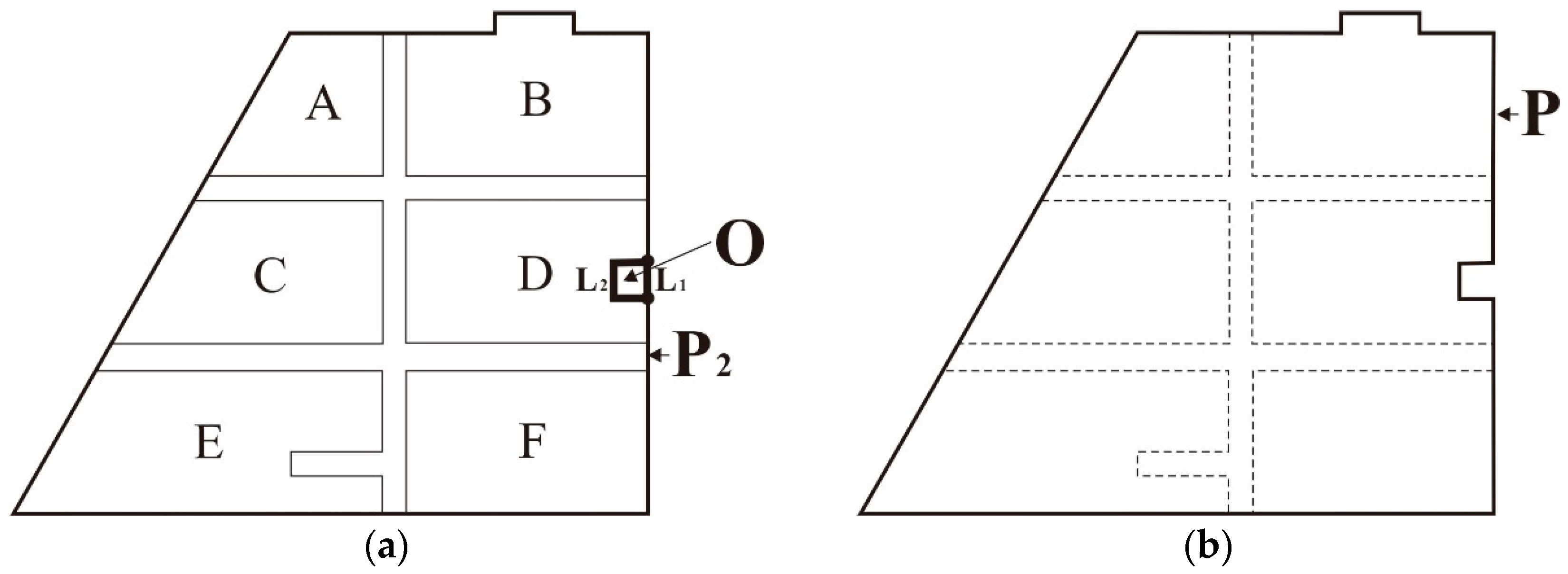
Because concave smoothing leads to inaccurate external outlines, the next step in the agglomeration process is to restore these concave areas. To this end, a topological structure containing semantic information is constructed from the P2 polygon and the original area group; if the arc segments of a polygon contain only one type of semantic datum, or no semantic information at all, this polygon is then a concave area that is removed during morphological erosion. In this case, an arc segment that possesses semantic information is used to replace the arc segment without semantic information to form a new area-group boundary polygon, P. This polygon is the minimum bounding polygon for the agglomeration area and its boundaries correspond to the external boundary outlines of the agglomeration area. Figure 14a shows a topological polygon, O, comprising of the arc segments, L1 and L2. L2 contains the semantic information of polygon D; however, because L1 is an arc segment in P2, it does not contain any semantic information. Polygon O may, therefore, be determined to be a concave area, and L2 is used to replace L1 as an arc segment in the boundary, P, which yields the boundary contour, P, as shown in Figure 14b.
3.3.2. Extraction of Agglomeration Lines
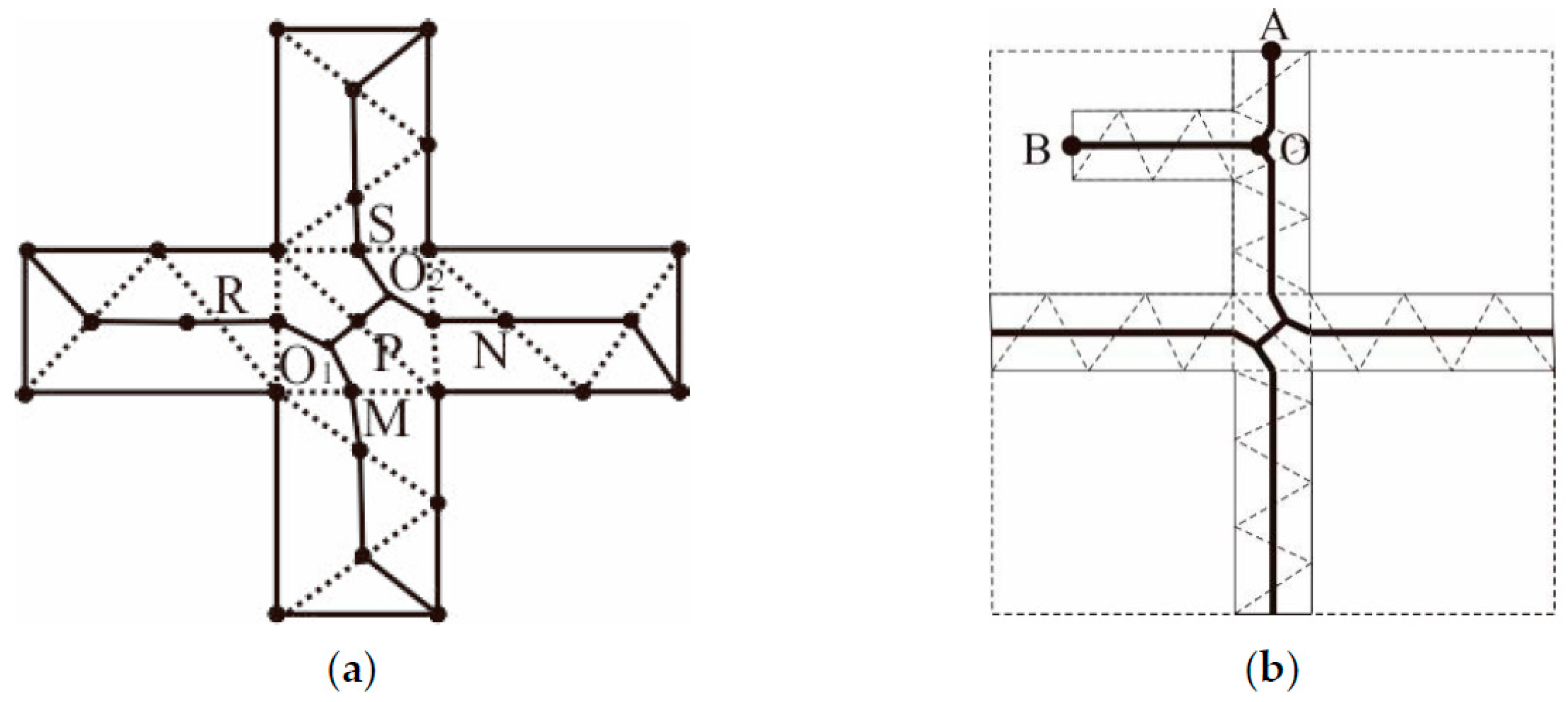
The bridging areas in an original area group are extracted by performing a spatial overlaying operation between the external boundary outlines of the agglomeration area and the original area group. By updating the topological relationships of the agglomeration area, the bridging areas can be converted into operable bridging area elements, as shown in Figure 15a. Then, the skeleton of the bridging area elements can be computed. The skeleton, which accurately reflects the main extension direction and primary shape features of the bridging areas, and terminal nodes exist along the external boundary outlines at the same time and may be used as the agglomeration line.
Although the use of boundary-constrained Delaunay triangulation for skeleton extraction in existing studies does produce skeletons that reflect the main extension direction and primary shape features of bridging areas, these skeletons suffer from the following two shortcomings when used as agglomeration lines:
- (1)
- Bridging areas are usually regular in shape, similar in width, and straight. However, most of their branches intersect with one another to form “+”-shaped junctions, leading to Y-shaped jitter that are very likely to occur in these areas due to the aggregation of type III triangles, as depicted in Figure 15a.
- (2)
- The concave and convex structures of bridging areas tends to induce errors during the extraction of agglomeration lines. In Figure 15b, it is shown that, if the main skeleton is extracted based on the SL or triangular area occupied by a skeleton, the OB skeleton, which corresponds to a concave structure, replaces the OA skeleton and becomes the main agglomeration line. Obviously, the extracted agglomeration line is not reasonable because the terminal node is not located on the boundary due to the influence of the concave area.
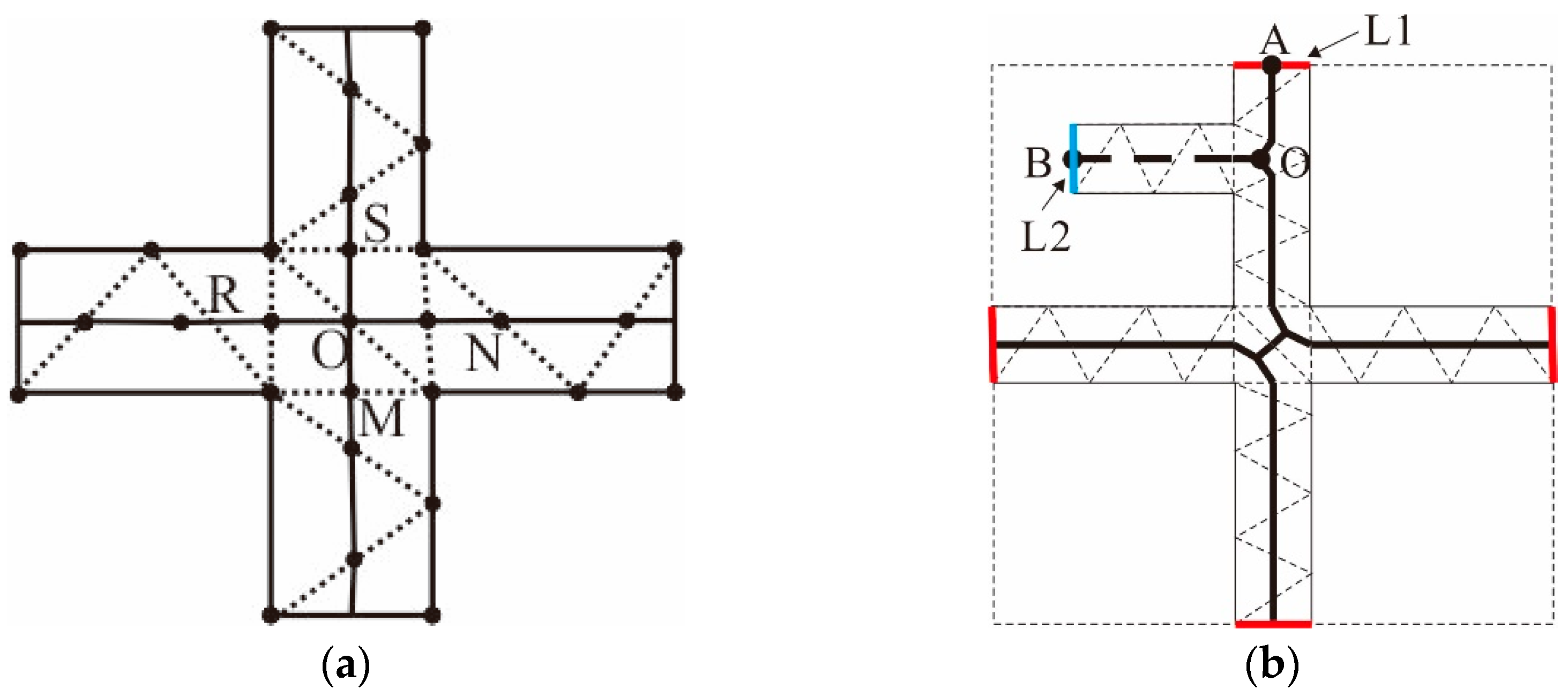
To rectify shortcoming (1), many studies have been performed on the removal of jitters from branch convergence zones. In this paper, the method proposed by Haunert and Sester [20], which is based on the reconstruction of junctions, is used to correct jitters. The extension direction of the main skeleton line is also used to adjust the terminal skeletons, as shown in Figure 16a.
For shortcoming (2), the agglomeration line is corrected by using boundaries as constraints in this work. Firstly, a semantic topology is constructed for the bridging areas and the original area group. Then, if an arc segment does not have semantic information and belongs to the arcs of the bridging areas, it is deemed as a boundary arc, and the skeleton connected to this arc is prioritized for preservation. Otherwise, if the terminal node of a dangling arc does not lie on the boundary, the arc is removed. In Figure 16b, it is shown that node A lies on L1, which is one of the boundary arcs; thus, the OA skeleton is preserved. Conversely, node B lies on a non-boundary arc, L2; thus, the OB skeleton is removed.
3.3.3. Progressive Process for the Agglomeration Operation
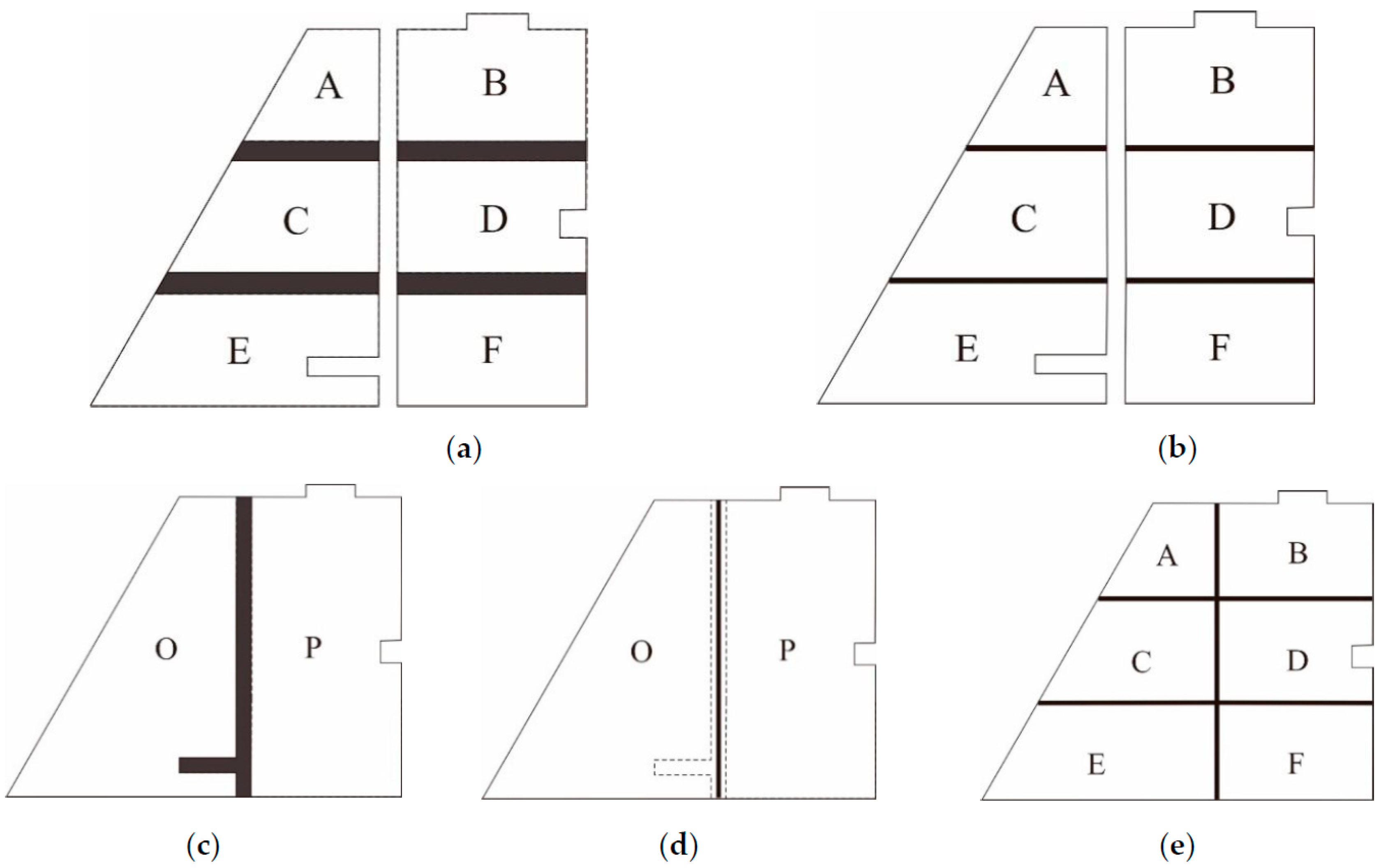
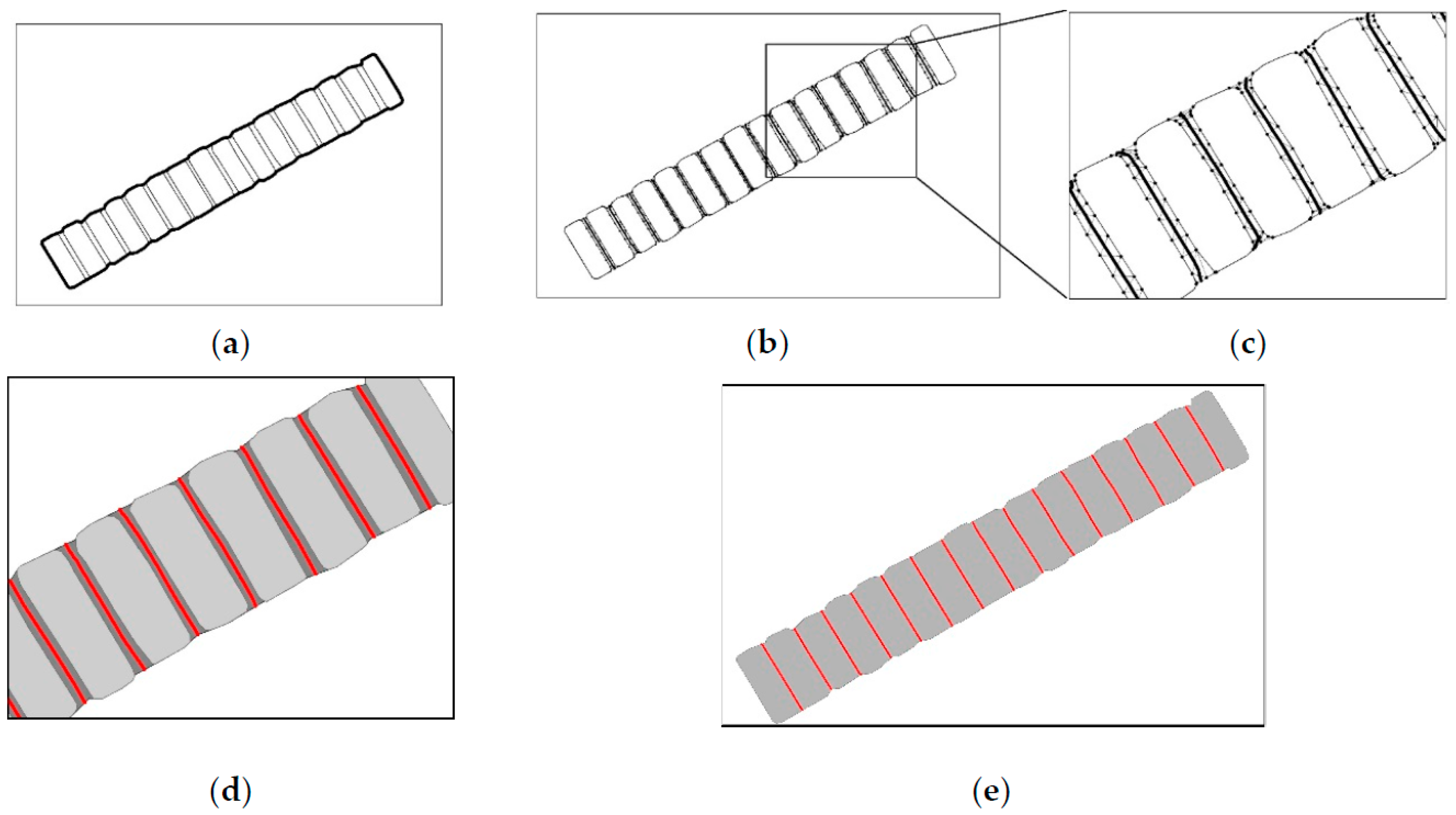
The extraction of agglomeration lines is first performed on the automatically identified agglomeration areas, which is followed by the agglomeration operation. The resulting area of this agglomeration operation and other area elements within the region are then used to construct new agglomeration areas for another round of agglomeration. This process is repeated until there are no longer any areas remaining that fulfill the conditions for agglomeration. Using the original area group, shown in Figure 13a, as an example, area elements A, B, C, D, E, and F form the candidate agglomeration areas, and the areas formed by A, C, and E and B, D, and F are identified as first-stage agglomeration areas, according to the criteria for agglomeration area identification. The bridging areas of these elements are then computed, as shown by the dark sections in Figure 17a. The agglomeration lines for the bridging areas are then extracted and the bridging areas are fused with the adjacent area elements, which yields the results for the first-stage agglomeration (shown in Figure 17b). Area O, which is the agglomeration result of elements A, C, and E, and area P, which is the agglomeration result of elements B, D, and F, are then judged according to the agglomeration criteria for the next step. As the two areas fulfill the criteria for agglomeration, a second-stage agglomeration is performed on them. The bridging areas produced by this process are shown by the dark sections in Figure 17c, and the agglomeration line of the bridging area is shown by the bold line in Figure 17d. The agglomeration lines from each stage are then extensionally connected to obtain the final result for agglomeration, which is shown in Figure 17e.
4. Experiment and Results
4.1. Experimental Data and Environment
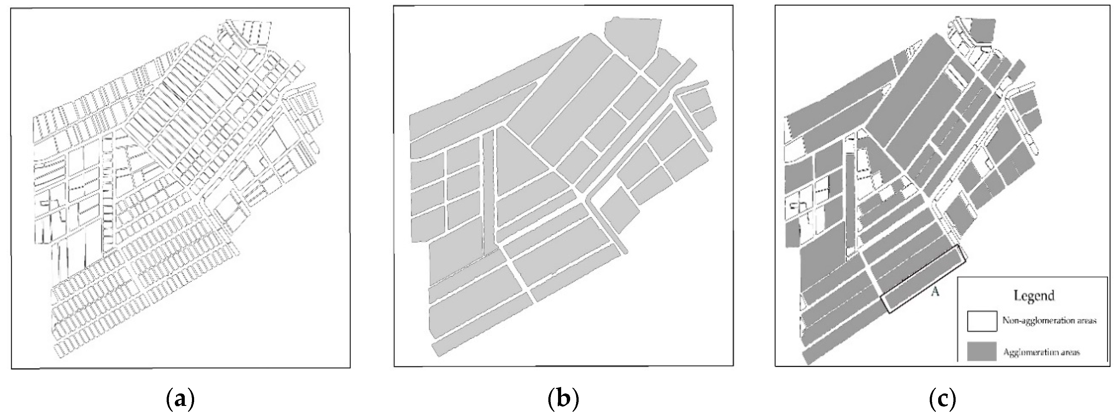
In this study, the proposed agglomeration method was embedded in the WJ-III mapping workstation developed by the Chinese Academy of Surveying and Mapping. The rationality and effectiveness of the method was then evaluated using a group of ponds. The experimental data used were census data for actual Chinese geographical conditions in a typical region in the Jiangsu Province (see Figure 18a), which has an aquaculture industry and a dense distribution of regularly arranged ponds with diverse shapes. The spatial distribution characteristics of this region were highly representative. The spatial range of the data was 2.8 × 3.1 km2, and the original scale was 1:10,000, whereas the target scale was 1:50,000. The experiments were conducted on an Intel Core I7-3770 CPU running at 3.2 GHz, with 16 GB of RAM and a 1024 GB solid-state disk. The operating system was Windows 7 (64-bit).
4.2. Results of the Agglomeration Operation
The width threshold of the bridging areas was calculated to be 20 m according to Equation (2). The 36 candidate agglomeration areas that were identified by the width threshold are shown in Figure 18b. The first-stage agglomeration area was subsequently obtained by calculating the DPI, SSI, and OI of all elements within the candidate agglomeration areas, as shown in Figure 18c.
The agglomeration process is described using the agglomeration area, indicated by rectangle A in Figure 18c, in the following example:
- (1)
- A dilation-erosion transformation was first performed on the original agglomeration area group and its external boundary outline was identified, as shown in Figure 19a.
- (2)
- The original data and boundary contours were overlaid to obtain the bridging areas, followed by node densification along the bridging area boundaries and boundary-constrained Delaunay triangulation to extract the main skeleton of the bridging areas, as shown in Figure 19b.
- (3)
- The terminal nodes of the main skeleton were then adjusted, while the boundaries were used as constraints for skeleton corrections to obtain the agglomeration lines, as shown by the red line in Figure 19c.
- (4)
- Based on these agglomeration lines, the bridging areas were amalgamated to obtain the agglomeration result shown in Figure 19d.
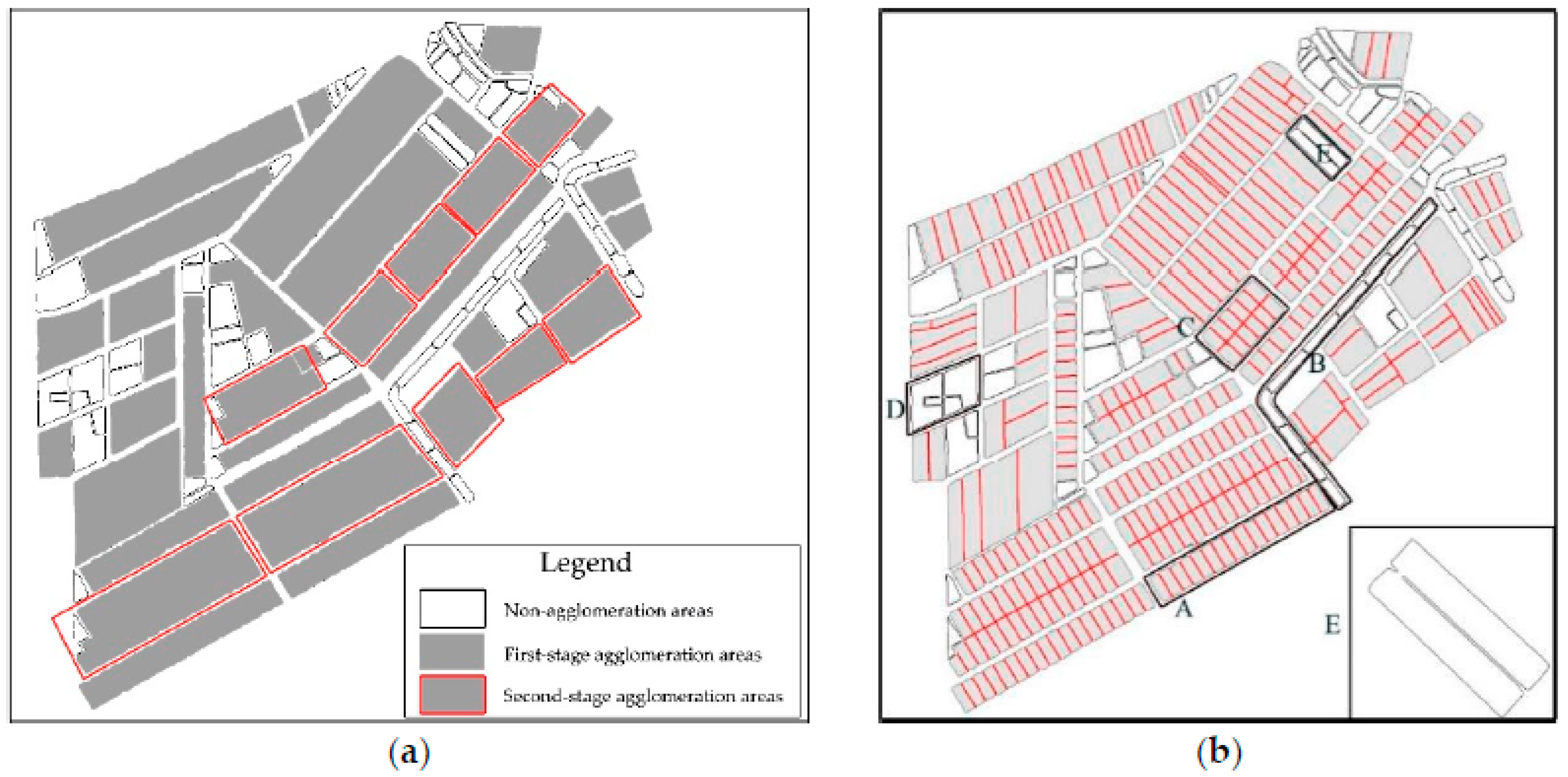
The results of the first-stage agglomeration and other area elements within the region were used to construct the second-stage agglomeration areas (i.e., the areas outlined by red rectangles in Figure 20a). All of the elements within the region were processed until this stage. Figure 20b illustrates the overall result of the agglomeration of the experimental data. In this figure, it is clear that the aggregation areas identified, based on typical characteristics, have accurate external boundary outlines and natural and smooth internal skeletons. The agglomerated pond area groups retain the spatial distribution characteristics of the original area groups, with originally separated elements that were aggregated, which highlights the aggregated nature of these elements (examples include agglomeration areas A and C). Area C, in particular, has undergone two stages of agglomeration. The proposed method is, therefore, highly effective for processing identified agglomeration areas. However, some of the elements were not agglomerated in the experiment for the following reasons:
- (1)
- Noncompliance with side-adjacency criteria (OI): By using candidate area B as an example, the elements within this area are highly similar in shape and are linearly ordered. However, these elements are side-adjacent along their shorter edge; thus, they were deemed unsuitable for agglomeration.
- (2)
- Noncompliance with shape similarity criteria (SSI): For example, although the elements in candidate area D superficially appeared to have the same overall shape, they were different based on their internal structure details. Area D was, therefore, deemed unsuitable for agglomeration due to the low shape similarity of its elements.
- (3)
- Element E was not agglomerated despite the overall shape of E being similar to that of its adjacent element because the identification of this element (for agglomeration suitability) was affected by the presence of a deep concave area inside the element. This result is a special case in the agglomeration process, and its treatment will require further study.
5. Discussion and Conclusions
Agglomeration is a core operation in the automated generalization of aggregated area groups. Traditional methods lack the process of identifying agglomeration areas and these methods can only be used by experienced cartographers with knowledge of the rules of generalization. In contrast, we have perfected the process of identifying agglomeration areas and attempted to use mathematical and statistical methods to perform agglomeration operations automatically. Therefore, in the proposed method, agglomeration areas were first identified based on typical characteristics, including the widths of striped bridging areas, DPI, SSI, and OI. These steps are followed by progressive agglomeration operations based on the computation of external boundary outlines and agglomeration line extraction and correction.
The results of the experiment, conducted using actual data, verify that the proposed method can accurately identify agglomeration areas and determine the range of agglomeration. The agglomeration lines extracted using the proposed method exhibit excellent connectivity and topological consistency. Furthermore, these agglomeration operations preserve the spatial distribution characteristics of the original area groups. Therefore, this study effectively complements conventional methods.
For future work, the range of agglomeration areas is extremely sensitive to the threshold values selected for the width of striped bridging areas, DPI, SSI, and OI. In this paper, we determine these threshold values based on a large number of experiments. However, studies on how to determine the appropriate threshold values are not proposed here. Therefore, further research on the selection of threshold values in different regions must be performed.
Author Contributions
C.L. conceived the original idea for the study, and all coauthors conceived and designed the methodology. Y.Y. conducted the processing and analysis of the data; C.L., X.L., and P.W. drafted the manuscript. All authors read and approved the final manuscript.
Acknowledgments
This research was funded by a project supported by the National Key Research and Development Program of China (Grant No. 2016YFF0201301). We are grateful to the National Geomatics Center of China for providing the data.
Conflicts of Interest
The authors declare no conflicts of interest.
References
- Haunert, J.H.; Wolff, A. Area aggregation in map generalisation by mixed-integer programming. Int. J. Geogr. Inf. Sci. 2010, 24, 1871–1897. [Google Scholar] [CrossRef]
- Cheng, T.; Li, Z. Toward quantitative measures for the semantic quality of polygon generalization. Cartogr. Int. J. Geogr. Inf. Geovis. 2006, 41, 135–148. [Google Scholar] [CrossRef]
- Zhou, X.; Truffet, D.; Han, J. Efficient polygon amalgamation methods for spatial OLAP and spatial data mining. In International Symposium on Spatial Databases; Springer: Berlin/Heidelberg, German, 1999; pp. 167–187. [Google Scholar]
- Regnauld, N. Algorithms for the amalgamation of topographic data. In Proceedings of the 21st International Cartographic Conference, Durban, South Africa, 10–16 August 2003; p. 1016. [Google Scholar]
- Delucia, A.A.; Black, R.B. A comprehensive approach to automatic feature generalisation. In Proceedings of the 13th International Cartographic Conference, Morelia, Mexico, 12–22 October 1987; pp. 169–192. [Google Scholar]
- Li, Z. Algorithmic Foundation of Multi-Scale Spatial Representation; CRC Press: Bacon Raton, FL, USA, 2006. [Google Scholar]
- Cheng, P.; Yan, H.; Han, Z. An algorithm for computing the minimum area bounding rectangle of an arbitrary polygon. J. Eng. Graph. 2008, 1, 122–126. [Google Scholar]
- Ruas, A. Multiple paradigms for automating map generalisation: Geometry, topology, hierarchical partitioning and local triangulation. In Proceedings of the ACSM/ASPRS Annual Convention and Exposition, Charlotte, North Carolina, 27 February–2 March 1995; pp. 69–78. [Google Scholar]
- Ware, J.M.; Jones, C.B.; Bundy, G.L. A triangulated spatial model for cartographic generalisation of areal objects. In Advances in GIS Research II (the 7th Int. Symposium on Spatial Data Handling); Kraak, M.J., Molenaar, M., Eds.; Taylor & Francis: London, UK, 1997; pp. 173–192. [Google Scholar]
- Cao, T.; Edelsbrunner, H.; Tan, T. Proof of correctness of the digital Delaunay triangulation algorithm. Comput. Geom. Theory Appl. 2015, 48, 507–519. [Google Scholar] [CrossRef]
- Yu, W. Assessing the implications of the recent community opening policy on the street centrality in China: A GIS-Based method and case study. Appl. Geogr. 2017, 89, 61–76. [Google Scholar] [CrossRef]
- Technical Specification for Resulting Map of National Census Geography; GDPJ 17-2016; Leading Group Office of the First National Census Geography of the State Council: Beijing, China, 2016.
- Penninga, F.; Verbree, E.; Quak, W.; van Oosterom, P. Construction of the planar partition postal code map based on cadastral registration. GeoInformatica 2005, 9, 181–204. [Google Scholar] [CrossRef]
- Mitropoulos, V.; Xydia, A.; Nakos, B.; Vescoukis, V. The use of epsilonconvex area for attributing bends along a cartographic line. In Proceedings of the International Cartographic Conference, A Coruňa, Spain, 9–16 July 2005. [Google Scholar]
- Gabay, Y.; Doytsher, Y. Automatic adjustment of line maps. In Proceedings of the GIS/LIS, Phoenix, Arizona, 25–27 October 1994; Volume 94, pp. 332–340. [Google Scholar]
- Douglas, D.H.; Peucker, T.K. Algorithms for the reduction of the number of points required to represent a digitized line or caricature. Can. Cartogr. 1973, 10, 112–122. [Google Scholar] [CrossRef]
- Zou, J.J.; Yan, H. Skeletonization of ribbon-like shapes based on regularity and singularity analyses. IEEE Trans. Syst. Man Cybern. B Cybern. 2001, 31, 401–407. [Google Scholar] [PubMed]
- Morrison, P.; Zou, J.J. Triangle refinement in a constrained Delaunay triangulation skeleton. Pattern Recognit. 2007, 40, 2754–2765. [Google Scholar] [CrossRef]
- Serna, A.; Marcotegui, B. Detection, segmentation and classification of 3D urban objects using mathematical morphology and supervised learning. ISPRS J. Photogramm. Remote Sens. 2014, 93, 243–255. [Google Scholar] [CrossRef] [Green Version]
- Haunert, J.H.; Sester, M. Area collapse and road centerlines based on straight skeletons. GeoInformatica 2008, 12, 169–191. [Google Scholar] [CrossRef]
Figure 1.
Agglomeration of vector polygons: (a) Original graphic; (b) supplementation of the original graphic; (c) skeleton of the supplementation; and (d) final result.
Figure 1.
Agglomeration of vector polygons: (a) Original graphic; (b) supplementation of the original graphic; (c) skeleton of the supplementation; and (d) final result.

Figure 2.
Minimum area-bounding rectangle (MABR) of an area group: (a) Original area group and (b) corresponding MABR.
Figure 2.
Minimum area-bounding rectangle (MABR) of an area group: (a) Original area group and (b) corresponding MABR.

Figure 3.
Framework for the proposed method.

Figure 4.
Boundary of an aggregated area group: (a) Original map and (b) MBR boundary.

Figure 5.
Adding Steiner nodes: (a) Original nodes of the area elements and (b) Steiner nodes.

Figure 6.
Distance calculation: (a) Boundary-constrained Delaunay triangulation and (b) height of a triangle between adjacent elements.
Figure 6.
Distance calculation: (a) Boundary-constrained Delaunay triangulation and (b) height of a triangle between adjacent elements.

Figure 7.
Internal structure characteristics of adjacent elements: (a) Sum of widths > BDistance and (b) sum of widths < BDistance.
Figure 7.
Internal structure characteristics of adjacent elements: (a) Sum of widths > BDistance and (b) sum of widths < BDistance.

Figure 8.
Calculating the average width of an area element: (a) Area element and (b) baseline of an area element.
Figure 8.
Calculating the average width of an area element: (a) Area element and (b) baseline of an area element.

Figure 9.
Adjacency of adjacent area elements: (a) Side-adjacency along longer edges and (b) side-adjacency along shorter edges.
Figure 9.
Adjacency of adjacent area elements: (a) Side-adjacency along longer edges and (b) side-adjacency along shorter edges.

Figure 10.
Calculation for the overlap degree index (OI): (a) 0≤ OI ≤ 1 and (b) OI =1.

Figure 11.
Three situations where OI = 0: (a) Parallel and non-overlapping; (b) orthogonality and (c) collineation.
Figure 11.
Three situations where OI = 0: (a) Parallel and non-overlapping; (b) orthogonality and (c) collineation.

Figure 12.
Flow chart of the progressive agglomeration operation.

Figure 13.
Dilation and erosion transformations: (a) Original map; (b) dilation transformation and (c) erosion transformation.
Figure 13.
Dilation and erosion transformations: (a) Original map; (b) dilation transformation and (c) erosion transformation.

Figure 14.
Restoration of concave areas: (a) Concave area based on semantic topology and (b) peripheral boundary contour of an agglomeration area.
Figure 14.
Restoration of concave areas: (a) Concave area based on semantic topology and (b) peripheral boundary contour of an agglomeration area.

Figure 15.
Issues arising from the use of the main skeleton line as the agglomeration line: (a) Fluctuations in the junction and (b) inaccurate extraction of terminal nodes.
Figure 15.
Issues arising from the use of the main skeleton line as the agglomeration line: (a) Fluctuations in the junction and (b) inaccurate extraction of terminal nodes.

Figure 16.
Adjustment of the agglomeration lines: (a) Adjustment of the fluctuations in the junction and (b) adjustment of terminal nodes.
Figure 16.
Adjustment of the agglomeration lines: (a) Adjustment of the fluctuations in the junction and (b) adjustment of terminal nodes.

Figure 17.
Progressive method for agglomeration. (a) 1st stage: Compute the bridging areas; (b) 1st stage: Generate the agglomeration lines; (c) 2nd stage: Compute the bridging areas; (d) 2nd stage: Generate the agglomeration lines and (e) final result of the agglomeration.
Figure 17.
Progressive method for agglomeration. (a) 1st stage: Compute the bridging areas; (b) 1st stage: Generate the agglomeration lines; (c) 2nd stage: Compute the bridging areas; (d) 2nd stage: Generate the agglomeration lines and (e) final result of the agglomeration.

Figure 18.
Identification and processing of the agglomeration areas: (a) Original pond data; (b) candidate agglomeration area and (c) first-stage agglomeration areas.
Figure 18.
Identification and processing of the agglomeration areas: (a) Original pond data; (b) candidate agglomeration area and (c) first-stage agglomeration areas.

Figure 19.
The agglomeration process: (a) Computation of the peripheral boundary contour, (b) extraction of the bridging area skeleton, (c) partial enlarged detail, (d) correction of the main skeleton and (e) result of the agglomeration.
Figure 19.
The agglomeration process: (a) Computation of the peripheral boundary contour, (b) extraction of the bridging area skeleton, (c) partial enlarged detail, (d) correction of the main skeleton and (e) result of the agglomeration.

Figure 20.
Experimental results: (a) Second-stage agglomeration areas and (b) overall results for the agglomeration of the experimental area.
Figure 20.
Experimental results: (a) Second-stage agglomeration areas and (b) overall results for the agglomeration of the experimental area.


Table 1.
Standard definition for the width of a long and narrow patch.
| Type | Map Width (mm) (1:500,000 > Scale > 1:10,000) |
|---|---|
| Roads | 0.4 |
| Rivers, canals and drains | 0.4 |
© 2018 by the authors. Licensee MDPI, Basel, Switzerland. This article is an open access article distributed under the terms and conditions of the Creative Commons Attribution (CC BY) license (http://creativecommons.org/licenses/by/4.0/).
Share and Cite
MDPI and ACS Style
Li, C.; Yin, Y.; Liu, X.; Wu, P. An Automated Processing Method for Agglomeration Areas. ISPRS Int. J. Geo-Inf. 2018, 7, 204. https://doi.org/10.3390/ijgi7060204
AMA Style
Li C, Yin Y, Liu X, Wu P. An Automated Processing Method for Agglomeration Areas. ISPRS International Journal of Geo-Information. 2018; 7(6):204. https://doi.org/10.3390/ijgi7060204
Chicago/Turabian StyleLi, Chengming, Yong Yin, Xiaoli Liu, and Pengda Wu. 2018. "An Automated Processing Method for Agglomeration Areas" ISPRS International Journal of Geo-Information 7, no. 6: 204. https://doi.org/10.3390/ijgi7060204
Note that from the first issue of 2016, this journal uses article numbers instead of page numbers. See further details here.