A Moment-Based Shape Similarity Measurement for Areal Entities in Geographical Vector Data


1
School of Remote Sensing and Information Engineering, Wuhan University, No. 129 Luoyu Road, Wuhan 430079, China
2
Zhejiang Academy of Surveying & Mapping, Zhejiang Innovation Base of Surveying and Mapping, West wen’er Road, Yuhang District, Hangzhou 310012, China
3
College of Resources and Environmental Sciences, Hunan Normal University, No. 36 Lushan Road, Changsha 410081, China
4
Key Laboratory of Geospatial Big Data Mining and Application, Hunan Province, No. 36 Lushan Road, Changsha 410081, China
*
Author to whom correspondence should be addressed.
ISPRS Int. J. Geo-Inf. 2018, 7(6), 208; https://doi.org/10.3390/ijgi7060208
Submission received: 16 March 2018
/
Revised: 19 May 2018
/
Accepted: 27 May 2018
/
Published: 31 May 2018
Abstract
:Shape similarity measurement model is often used to solve shape-matching problems in geospatial data matching. It is widely used in geospatial data integration, conflation, updating and quality assessment. Many shape similarity measurements apply only to simple polygons. However, areal entities can be represented either by simple polygons, holed polygons or multipolygons in geospatial data. This paper proposes a new shape similarity measurement model that can be used for all kinds of polygons. In this method, convex hulls of polygons are used to extract boundary features of entities and local moment invariants are calculated to extract overall shape features of entities. Combined with convex hull and local moment invariants, polygons can be represented by convex hull moment invariant curves. Then, a shape descriptor is obtained by applying fast Fourier transform to convex hull moment invariant curves, and shape similarity between areal entities is measured by the shape descriptor. Through similarity measurement experiments of different lakes in multiple representations and matching experiments between two urban area datasets, results showed that the method could distinguish areal entities even if they are represented by different kinds of polygons.
1. Introduction
With the influences of data acquisition errors, map generalization, different application purposes and people’s explanatory differences, there are inconsistencies in the expression of real-world objects in different geospatial data [1,2,3]. Fast and accurate matching of the same entities from multi-source spatial data is one of the key technologies for geospatial data integration, conflation, updating, and quality assessment [4,5,6,7,8]. Commonly, all kinds of features will be used in matching entities. Matching methods can be divided into geometric matching, topology matching and semantic matching. Small differences of topological relations between two datasets may lead to different matching results, while semantic matching heavily relies on consistency and completeness of data properties [9]. As a result, geometric matching is used mostly. Commonly used geometric matching features include location, size, orientation, and shape [10,11]. Compared with location, size, and orientation, shape is less dependent on spatial position accuracy and it can distinguish objects more intuitively. Therefore, it is important to study the method of shape similarity measurement.
There are extensive methods of shape similarity measurement in image processing [12]. However, only some of them are suitable for vector data, because shape representation of vector polygons is different from images. Simply transforming vector polygons into images will introduce bias and require additional computation. Thus, scholars pay more attention to researching similarity measurement of areal entities in geographical vector data. Presently, commonly used shape description methods for vector polygons include the tangent space shape description method [5,13], multi-level chord length shape description function [14,15], shape context descriptor [16], and Fourier shape description method [17,18]. The tangent space method describes shape through tangent values of vertex angles on outlines of polygons. Not only can it realize shape matching between polygons, but also the matching between vertices on the polygons. However, it heavily relies on the starting point. The multi-level chord length method divides polygon contours by arc length. One dividing point and the vertexes on the polygon contour compose a chord length function. The multi-level chord length function is composed of several chord length functions and can be used to describe the shape. This method can measure overall similarity or local similarity between shapes in geospatial data at different scales, but it is time-consuming. The shape context descriptor extracts a global feature for each point on the boundary of polygons. It is often used to find the corresponding points on two polygons, but this method requires too many feature points. In Fourier shape description method, the distance from polygon contour to the center of the polygon forms a discrete sequence. Then, the Fourier shape descriptor is obtained by performing fast Fourier transform on the sequence. This method is simple and widely used, but it is easily affected by noise. In geographical vector data, there are not only simple polygons, but also complex polygons, such as holed polygons that are polygons with holes and multipolygons which are composed of several disjoint polygons [19]. However, the above methods are mainly applied to simple polygons, because they cannot describe relations between holes and relations between disjoint polygons. Xu et al. [18] proposed a method using Fourier descriptors to describe the exterior contour of holed polygons. Then, they described the structure of holes with position graph. Shape similarity between holed polygons is measured by Fourier descriptors and position graph. Chen et al. [20] proposed a hierarchical model to measure shape similarity between complex holed-region entities. They divided a complex entity into three layers: A complex scene, a micro-spatial-scene, and a simple entity. Then they calculated the similarity of three layers respectively. However, these two methods can only measure shape similarity between holed polygons and cannot be applied to simple polygons and multipolygons.
Areal entities have multiple representations in different geographical vector datasets. The same areal entities can be represented by either a simple polygon, a holed polygon or a multipolygon. Thus, it is necessary to find a similarity measurement that can apply to different kinds of polygons. Vector polygons are represented by points on their contours. Thus, most shape description methods used in Geographic Information System are contour-based. However, contour-based shape description may not be suitable for complex shapes that consist of several disjoint regions such as multipolygons [21]. In the field of traditional image processing, the moment description method has a wide range of applications in image matching, retrieval and identification [22]. This method can extract invariant shape features under the transformation of translation, rotation, and scaling, and can describe global shape features of overall areas which means it can describe all kinds of polygons [23]. Therefore, this region-based shape description method is more suitable for areal entities than methods based on shape contour description. Although shape representation of vector data is different from images, vector data can also express shape feature of entities. In this paper, the moment description method in the field of image processing is introduced to extract invariant moments of areal entities in vector data. Considering inconsistencies caused by map generalization, we construct convex hull moment invariant curves to make the shape description more robust. Then, shape descriptors are obtained by fast Fourier transform on the curves to realize the similarity measure of areal entities. Specifically, the contributions of this paper are summarized below.
- We extend the calculation of geometric moments from images to vector polygons.
- Based on convex hull and moment invariants, we construct convex hull moment invariant curves to describe shapes and extract shape descriptors from the curves.
- We validate our method by experiments of invariance, similarity, and matching. Experimental results show that our shape descriptor is invariant to translation, rotation, and scaling. In addition, it takes advantage of moment invariants and convex hull and can be used for vector data matching.
The rest of this paper is organized as follows. Section 2 introduces multiple representations of areal entities in geographical vector data. Section 3 introduces moment-based method of describing shape and discusses moment calculation method in geographical vector data. In Section 4, we propose a shape similarity measurement model considering map representation differences in geospatial datasets. Next, we apply the model to different experiments, then discuss and analyze the results in Section 5. Finally, we conclude the study in Section 6.
2. Areal Entities in Geographical Vector Data
In geographical vector data, polygons are usually used to represent areal entities. However, areal entities in the real world are complex in most cases. For example, the American territory includes several disjoint regions which are the mainland of the United States, Alaska, and the Hawaiian islands. There is a hole in the South African territory, because it completely contains Lesotho. Thus, simple polygons are difficult to fully describe complex areal entities [24]. Clementini et al. [25] divided polygons in geospatial data into simple polygons, holed polygons, and multipolygons. In addition, they gave detailed mathematical definitions of three types of polygons. Based on their definitions, we define polygons used in our paper as follows.
Definition 1.
Simple polygon:A simple polygon is a counterclockwise closed point set with connected interior and connected exterior. It can be expressed as
Definition 2.
Holed polygon:A holed polygon contains an outer contour and one or more inner contours. The outer contour is represented by a counterclockwise closed point set, and the contour of internal holes are represented by clockwise closed point sets. Thus, the holed polygon is expressed as, where O is the outer contour and I is the inner contour.
Definition 3.
Multipolygon:A multipolygon is composed of more than two disjoint regions, each of which consists of a simple polygon or a holed polygon, that is, M is a multipolygon, S is a simple polygon, and H is a holed polygon.
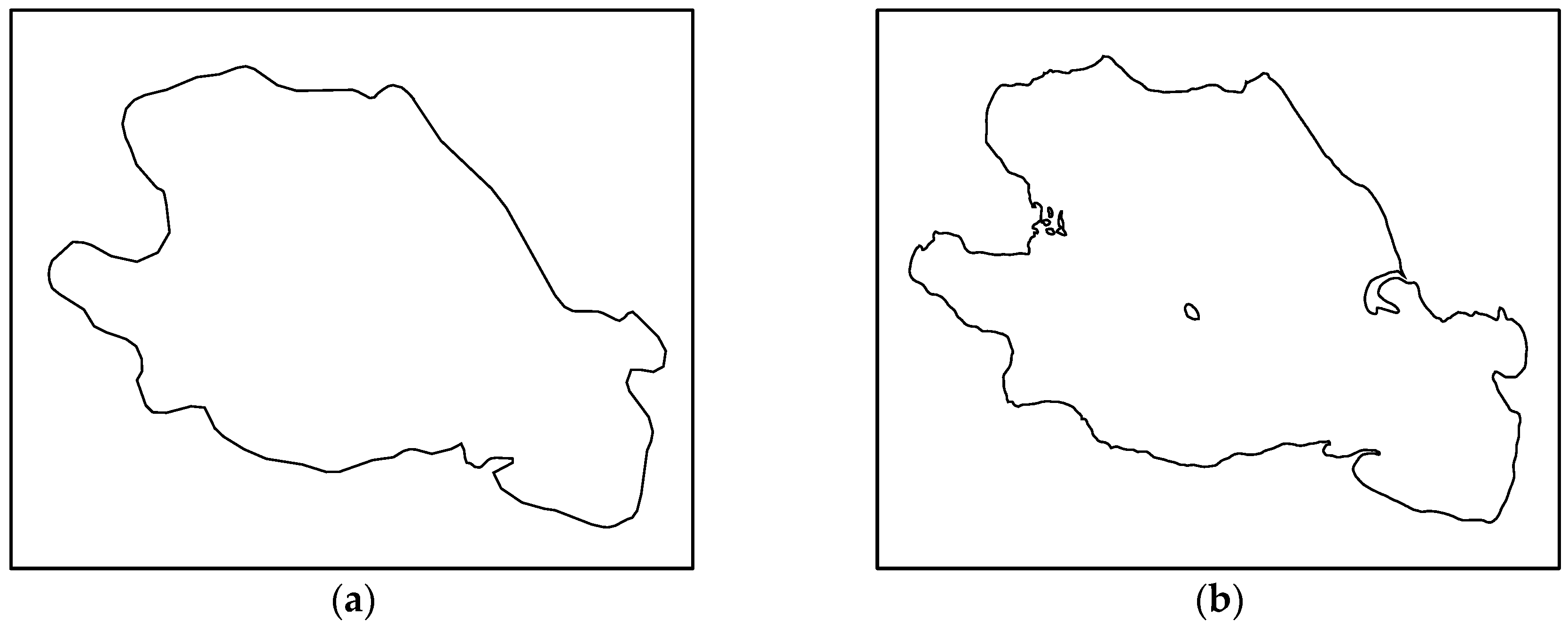
The same areal entities can be represented by different types of polygons (Figure 1). Thus, shape similarity between areal entities can be divided into six cases. There are similarities between two simple polygons, a simple polygon and a holed polygon, a simple polygon and a multipolygon, two holed polygons, a holed polygon and a multipolygon, and between two multipolygons Contour-based shape descriptors can only describe simple polygons, because they cannot describe holes in holed polygons and disjoint regions in multipolygons. However, region-based shape descriptors can describe simple polygons, holed polygons, and multipolygons with all of the cases above. Thus, region-based shape descriptors are more suitable for areal entities.
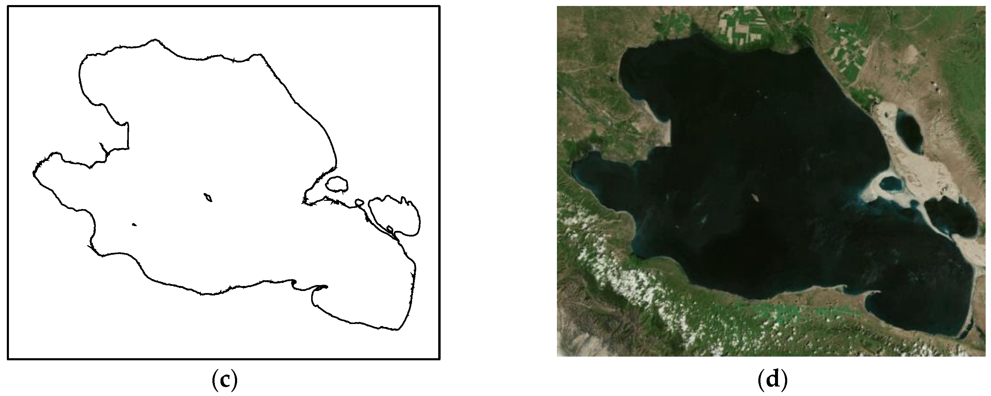
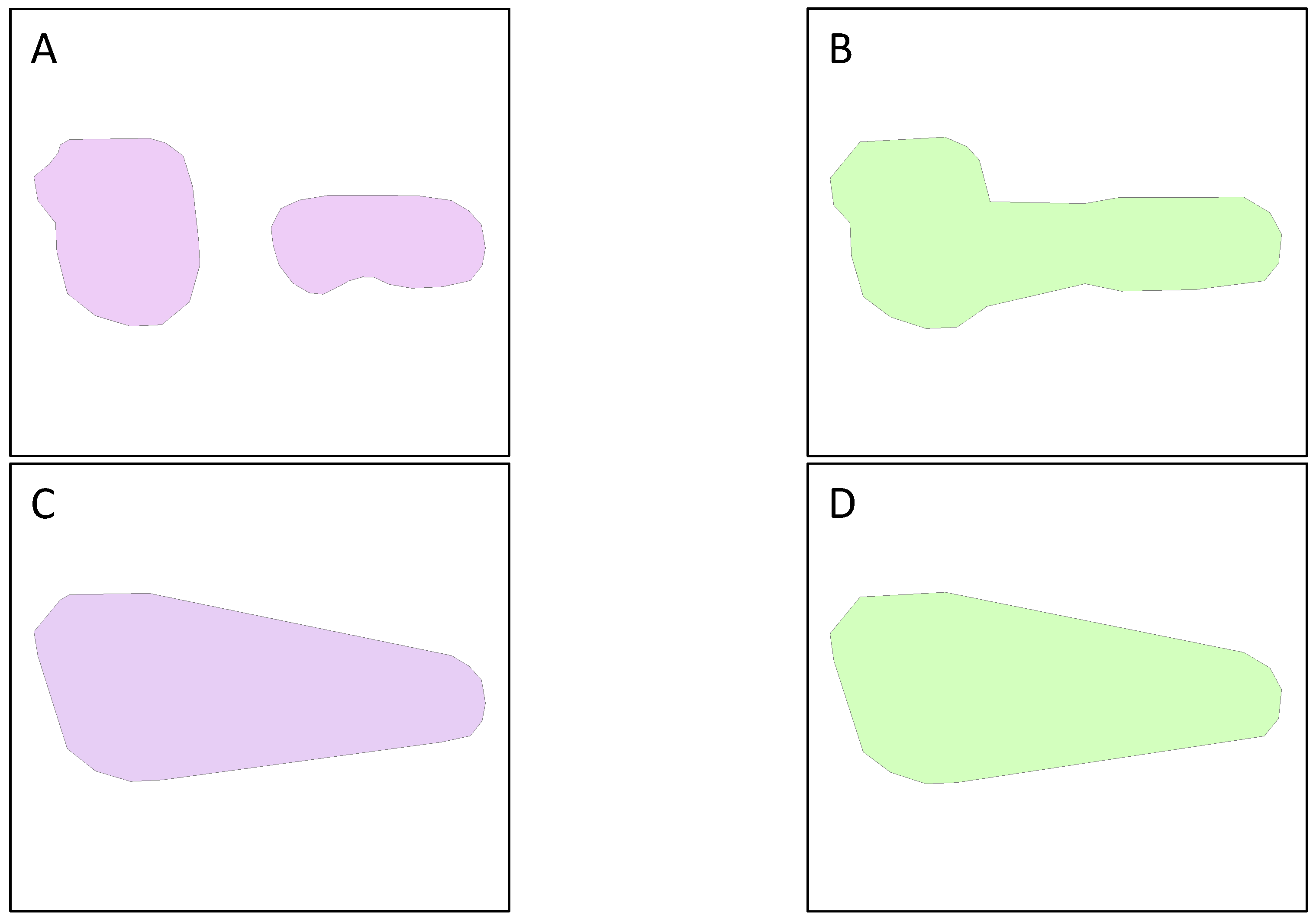
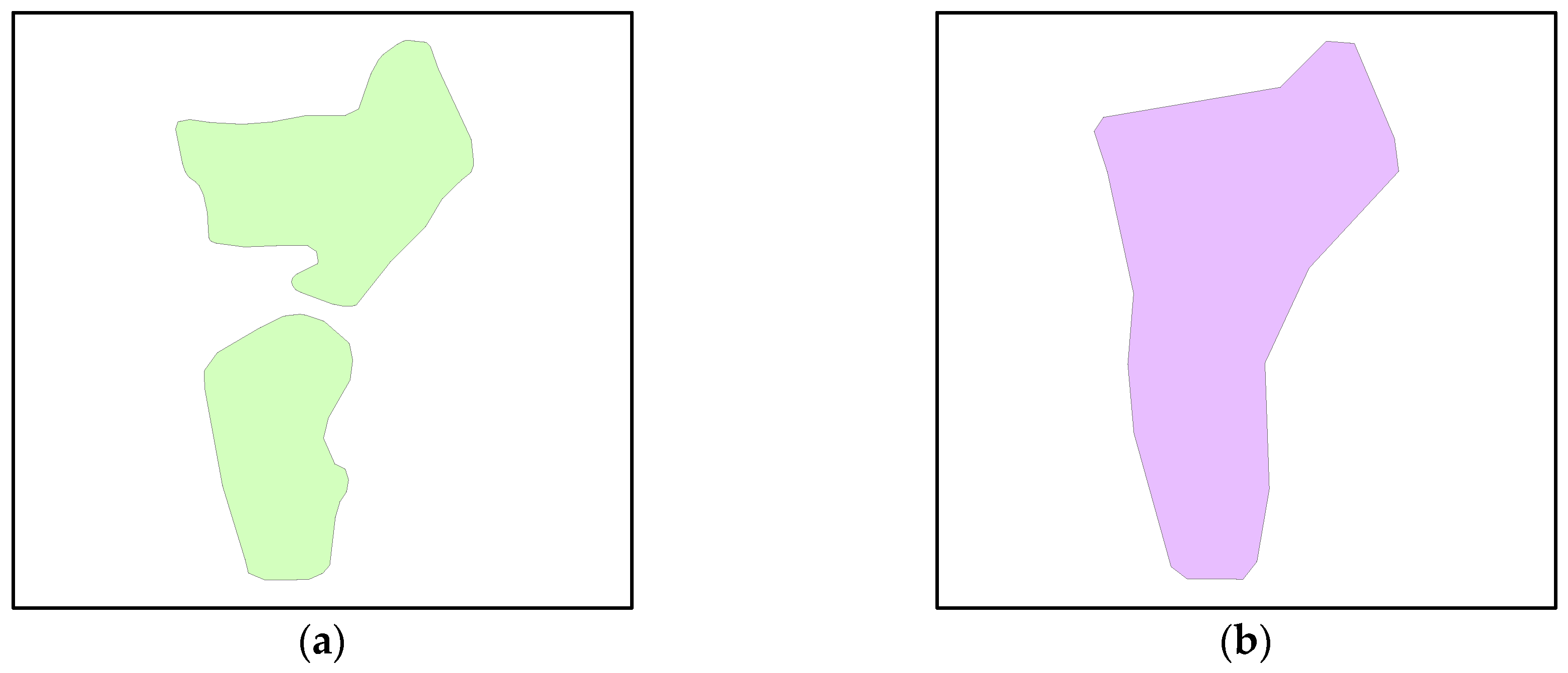
Affected by map generalization, shapes of the same areal entities may differ in multiscale data, while their convex hulls change slightly compared with shapes (Figure 2). In addition, convex hulls can combine disjoint regions into single region, which is convenient for the comparison between multipolygons and simple polygons or multipolygons and holed polygons. Convex hull is also a basic method of multi-scale representation of vector data [26]. Thus, we can use convex hull to extract boundary feature of vector polygons. On the other hand, convex hull can only describe the rough shape of polygons. Areal entities with totally different shapes may also have similar convex hull (Figure 3). Thus, it is necessary to find a shape similarity measurement to combine region-based shape descriptor with convex hull. Through the combination method, the same entities will have a higher similarity while different entities will have a lower similarity. There are many investigations in region-based shape description [27,28,29], while Hu moment invariants [30] is a simple and effective region-based method. It can be calculated by the contour of shape [31], which is suitable for vector polygons. In addition, it can extract global feature of different types of polygons and can be easily connected with convex hull. By combining Hu moment invariants with convex hull, we can measure shape similarity between areal entities.
3. Moments and Moment Invariants
3.1. Hu Moment Invariants in Images
The definition of moments is derived from the theory of probability, which is a numerical feature used to describe the distribution of random variables. Hu applied the theory of moments to image analysis to obtain moment invariants. If gray values of each pixel in an image are regarded as a two-dimensional density distribution function f(x,y), the (p + q)th order geometric moment of the image is defined as follows:
where ζ is the image region and f(x,y) is gray value of the pixel at xth row and yth column of the image. The moments can be used to describe characteristics of an image, but they are affected by coordinate transformation. Thus defining the (p + q)th order center moment of an image:
where are the center of the image, .
Then, defining the (p + q)th order normalized center moment of an image:
The normalized center moment has translational and scaled invariance, but does not have rotational invariance. Hu obtained a set of moment invariants with translational, rotational and scaled invariant features by linearly combining the lower order normalized center moments. The expressions are as follows:
All the moments and moment invariants are defined in continuous domain. However, they should be transformed to discrete domain in image processing. If the size of a discrete image is , then the (p + q)th order geometric moment in discrete domain is defined as follows:
Center moments, normalized center moments and Hu moment invariants can be derived from geometric moments in discrete domain.
3.2. Moments for Vector Polygons
Vector polygons defined in Section 2 are represented by point sets on their contours. Thus, we cannot calculate moments of polygons by the discrete form in Equation (5). It is necessary to extend the moment calculation method to vector polygons. In the continuous form of geometric moment, we can simply get the density distribution function f(x,y) of a vector polygon V as follows:
where ζ is the region of polygon V.
Therefore, the (p + q)th order geometric moment of a vector polygon can be expressed as:
Then, we need to calculate Equation (7) based on vertices on the polygon. Jiang et al. [31] proposed a polygonal approximation method to calculate geometric moments in images. In their method, they transform the double integral in Equation (7) into a line integral along the boundary of a simple polygon by applying the Green’s formula. Then, the line integral can be calculated by vertices on the polygon. Based on their method, we extend the geometric moment’s calculation method for different kinds of vector polygons. Detailed derivations of geometric moments for simple polygons, holed polygons, and multipolygons are given in the Appendix A. By modifying geometric moments of polygons, we can also get center moments, normalized center moments, and moment invariants of vector polygons.
4. Shape Description Model for Areal Entities
Moment invariants of polygons can describe translation, rotation, and scaling invariant features of the entire shape. However, it is easy to be influenced when describing the same entity at different scales, because there is map generalization in different scales. In order to get robust shape features under map generalization, we introduce convex hulls of polygons to construct the moment invariants feature description model.
Convex hull of points is the smallest convex polygon that contains the points. It is a basic structure that describes the shape of a spatial object. Additionally, it is usually less variable in the process of map generalization. Therefore, it has a wide range of applications in map generalization [26,32]. In this paper, we use the local moment invariant proposed by Zhao et al. [33] to make the convex hull vertices participate in the calculation of polygon’s moment invariants. Thus, we can obtain shape features that combine convex hull and moment invariants. The features are stable under the process of map generalization.
4.1. Local Moment Invariants of Complex Polygons
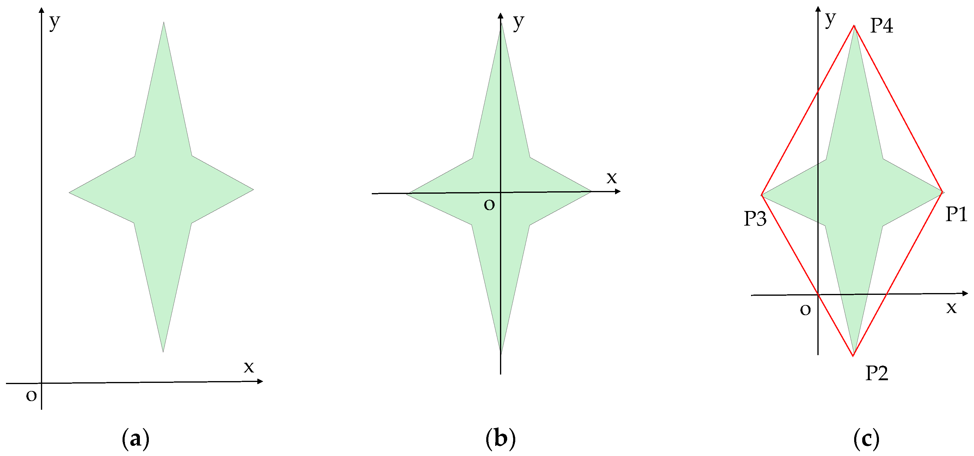
According to the definition of center moments, we can get moments that are invariant to translation by moving the origin of coordinates to the centroid of a polygon (Figure 4). After this transformation, geometric moments of the polygon are invariant to translation. Therefore, we can also move the origin of coordinates to an arbitrary point P(xi,yi) to get translation moment invariants. The arbitrary point P should be on the boundary of a polygon or on the boundary of the convex hull of a polygon. Zhao et al. [33] define the moment calculated by this method as local moment and define the point P as reference point of local moment. The (p + q)th order local moment relative to point P of a polygon can be expressed as follows:
We can prove the local moment is also invariant to translation. If (x,y) belongs to the polygon, and belongs to the polygon after translation of coordinates, then we can get the relation between (x,y) and :
The reference point P is also satisfied by Equation (9). Thus, the (p + q)th order local moment of the polygon after translation is Equation (10):
Equation (10) proves translation invariance of local moments. The same as Hu moment invariants of polygons, we can get seven local moment invariants by normalizing and linearly combining the low order local moments. They are also invariant under the transformation of translation, rotation, and scaling.
According to the definition, we can calculate the local moments relative to arbitrary points by geometric moments. Binomial decomposition of the integrand in Equation (8) is as follows:
The relationship between local moment and geometric moment can be obtained by substituting Equations (7) and (11) into Equation (8) respectively. Then, relationships between low order local moments and geometric moments can be easily deduced:
In the case of known geometric moments, by using Equation (12), we can quickly calculate local moment invariants of polygons relative to arbitrary points.
4.2. Convex Hull Moment Invariant Curves
We can take every convex hull vertex as reference point of local moment invariants. Therefore, every local moment invariant can extract global feature of polygons, and all of local moment invariants reference to convex hull vertices can represent the structure of convex hull of polygons.
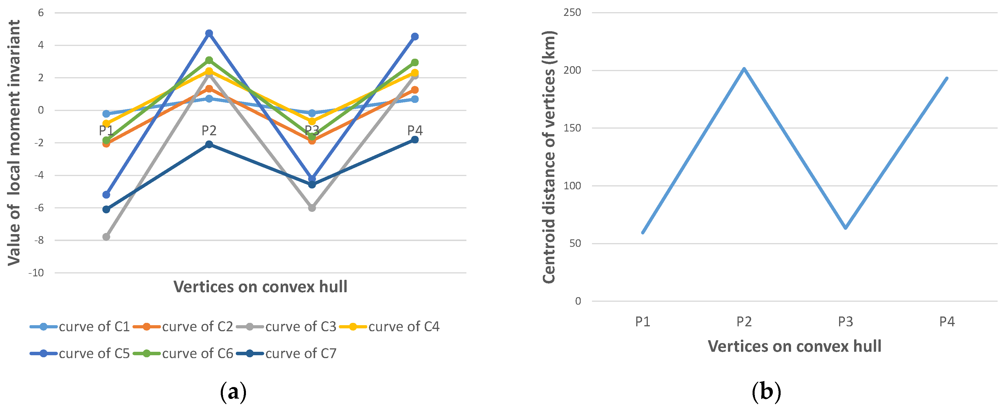
If X is convex hull of polygon C, it can be represented as a set of vertices . Then we can calculate seven local moment invariants taking the convex hull vertex as the reference point. If we take each vertex in X as the reference point successively, we can get seven sequences of local moment invariants. Each sequence can form a curve, which is called the convex hull moment invariant curve. Figure 5a is convex hull moment invariant curves of the polygon in Figure 4. Every point on the curve is a local moment invariant. Figure 5b is centroid distance of vertices on the convex hull. The centroid distance of vertices is the distance between the centroid of polygon and the convex hull vertices. It can be found that the shape of every convex hull moment invariant curve is similar to the centroid distance curve. In addition, the convex hull moment invariant curve is invariant to translation, rotation and scaling because of the invariance of every local moment invariant on the curve.
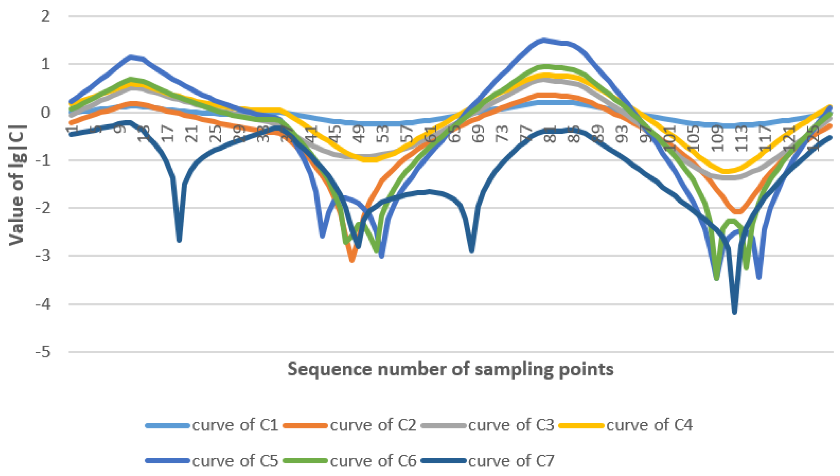
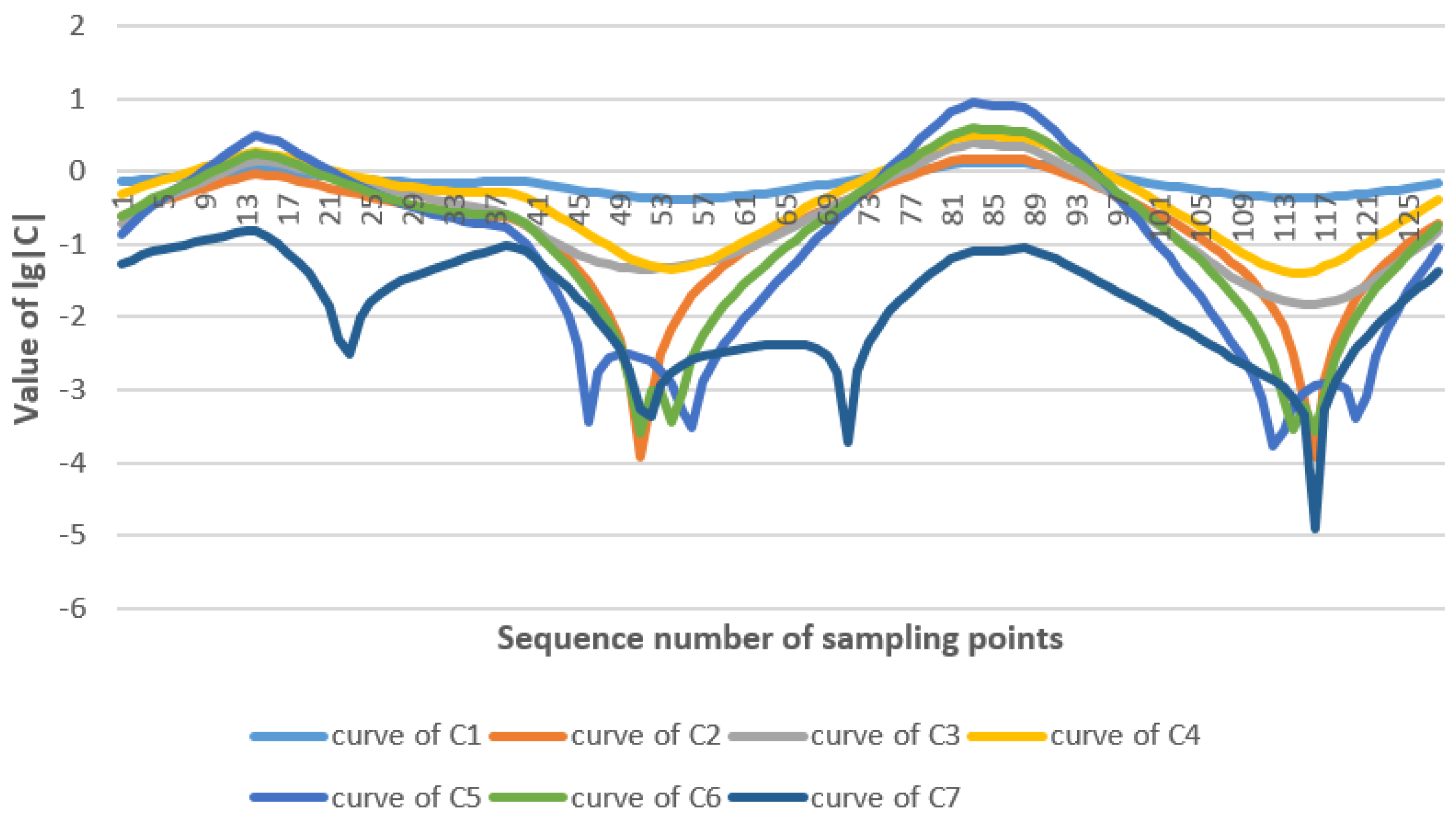
For the same lakes at different scales (Figure 6), we can get two series of convex hull moment invariant curves (Figure 7 and Figure 8). In order to make the curves more comparable, we resample the convex hull by arc length and take the logarithm of each local moment invariant. It can be found that the two series of curves are similar overall but vary in detail. These characteristics are generated by the method of combining moment invariants with convex hull. It can be used to measure the similarity between areal entities. However, there is displacement on the two series of curves, which is caused by the differences of the starting point on the convex hull. In addition, we can hardly get the similarity value of two lakes only by comparing the curves qualitatively. It is necessary to measure the similarity between areal entities quantitatively.
4.3. Feature Similarity Calculation
In order to eliminate the dependence of starting point on convex hull and get shape descriptors, we introduce the method of fast Fourier transform to extract features on convex hull moment invariant curves. First, convex hull of a polygon is resampled by arc length in power of 2. We can get the resampled vertices set , where m equals . Then, we can calculate seven local moment invariant sequences by taking each point in the resampled vertices as reference point. Performing fast Fourier transform to each sequence and selecting top k of the Fourier coefficient sequences after transformation, we can get seven feature vectors. The feature matrix composed by seven feature vectors is a shape descriptor of the polygon.
If and are the descriptors of two polygons respectively, and and are the elements in ith row and jth column of and . Then we can define the similarity between matrices to get the similarity between polygons.
where .
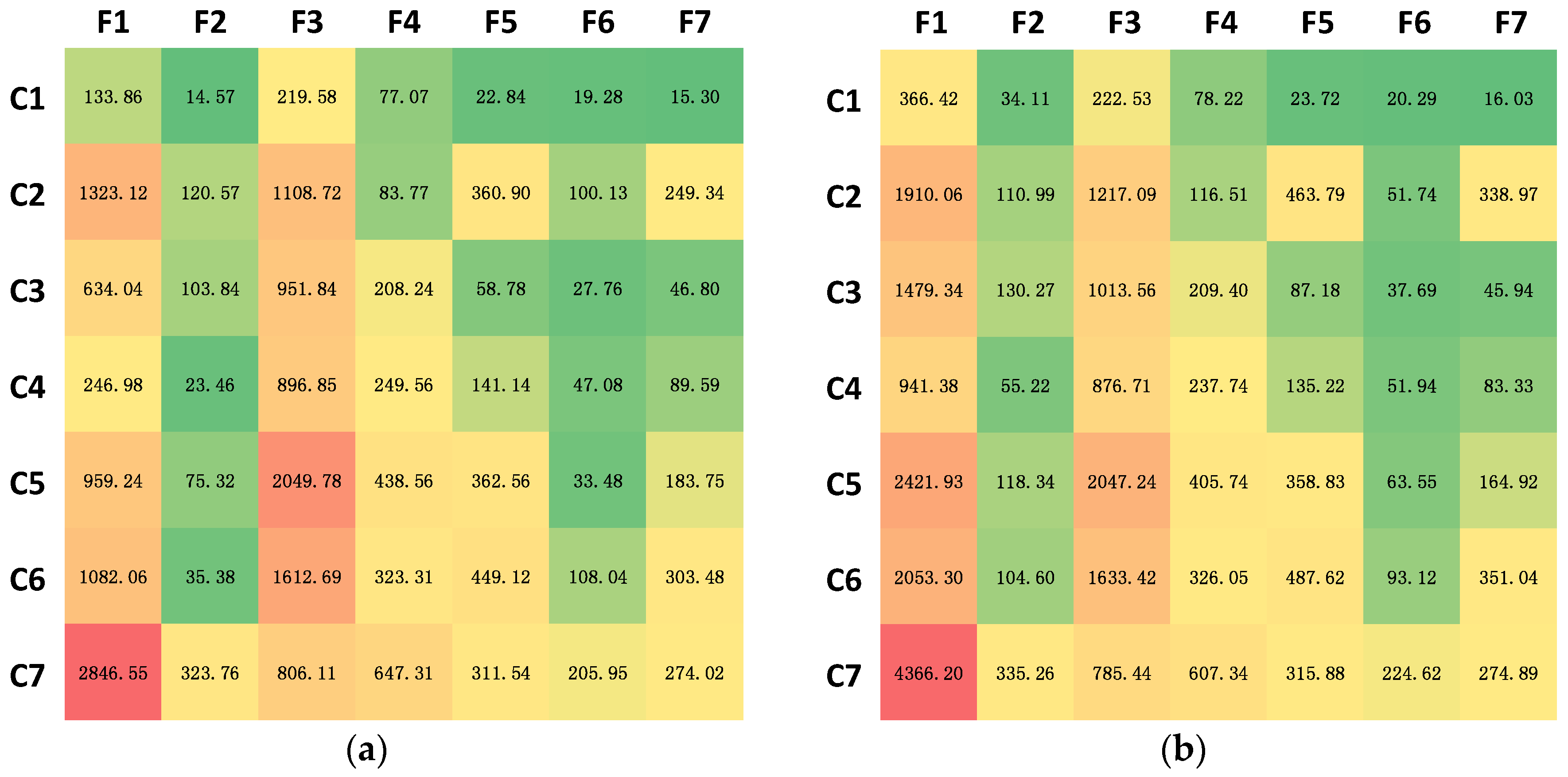
For the lakes in Figure 6, we resample the number of convex hull vertices to 256 and select top seven of the sequences after fast Fourier transform. Thus, we can get two shape descriptors for the two polygons (Figure 9). For visual comparison, we map the values of matrices to the color band. Higher values are colored with red while lower values are colored with green. In addition, we index each element in the matrix. The element with C1F1 means it is calculated by the first Hu moment invariant , and it is the first Fourier coefficient after fast Fourier transform. It can be found that the two shape descriptors are extremely similar. Then, we can get the similarity between two areal entities by Equation (13). The similarity between two lakes in Figure 6 is 0.8.
5. Experiments and Discussion
5.1. Experiment of Invariance
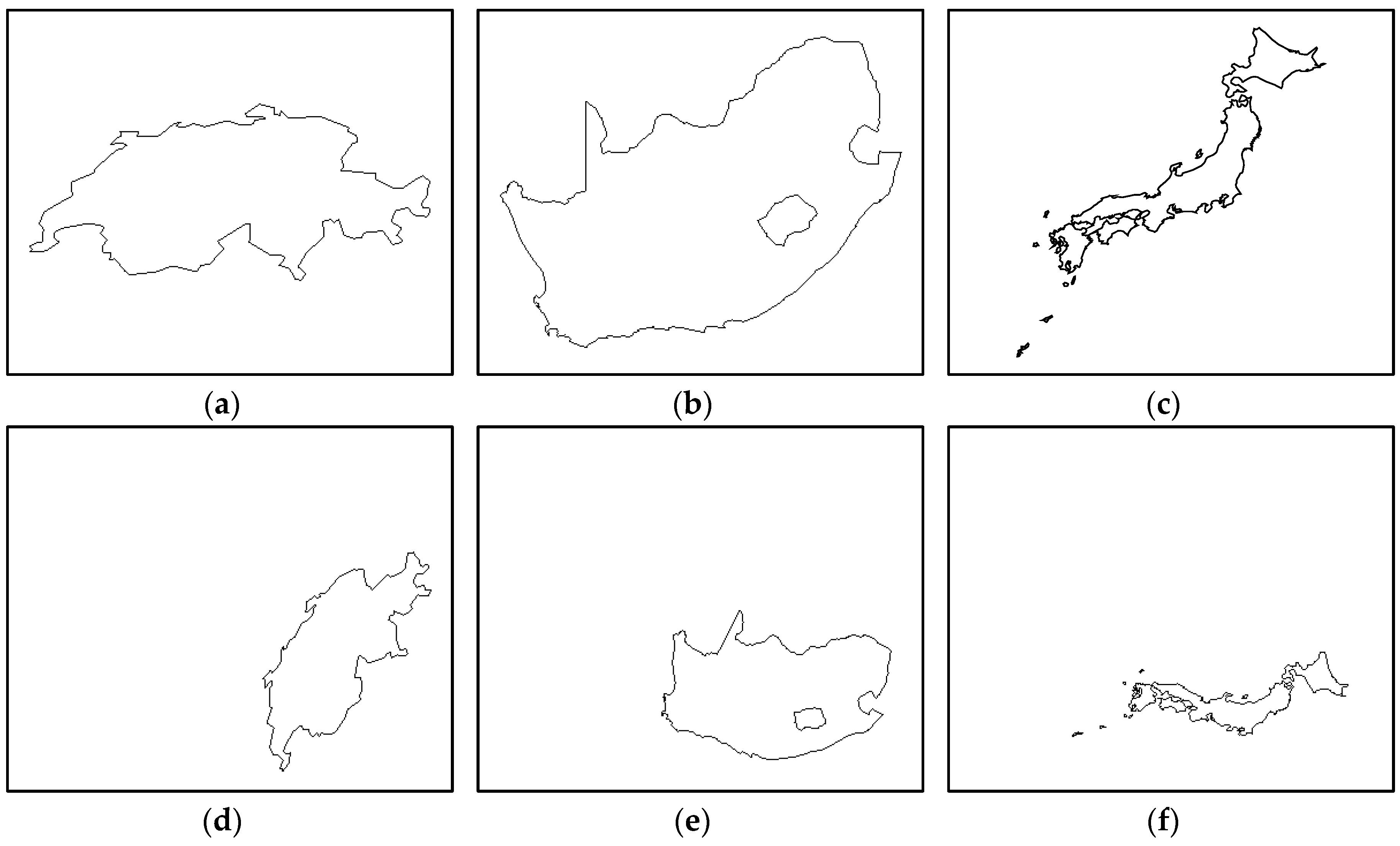
In this paper, we select three areal entities of different countries to prove the invariance of shape description methods. They are Switzerland, South Africa, and Japan. The first row in Figure 10 are the countries represented by simple polygon, holed polygon and multipolygon respectively. The second row in Figure 10 are transformational polygons by translating, rotating, and scaling the polygons in the first row. Then, we can get seven Hu moment invariants of different polygons by the calculation method we proposed in Section 3. The results are shown in Table 1. By comparing invariants between a and d, b and e, and c and f, we can find that Hu moment invariants calculated by our method are stable for coordinate transformation. In addition, the method is suitable for simple polygons, holed polygons, and multipolygons. We also calculate shape descriptors of six polygons by our method in Section 4. In the method, we set the parameter of sampling points number m to be 256, and set the parameter of Fourier coefficients number k to be 2. Then, we can get fourteen features for each polygon (Table 2). The result indicates that our shape descriptor is also stable under transformation of different types of polygons. Compared with Hu moment invariants, the shape descriptor requires two parameters. Less sample points result in incomplete description of shape and more number of Fourier coefficients may introduce high frequency noise. Thus, the shape descriptor only has translation, rotation and scaling invariance within a certain parameter range.
5.2. Experiment of Similarity
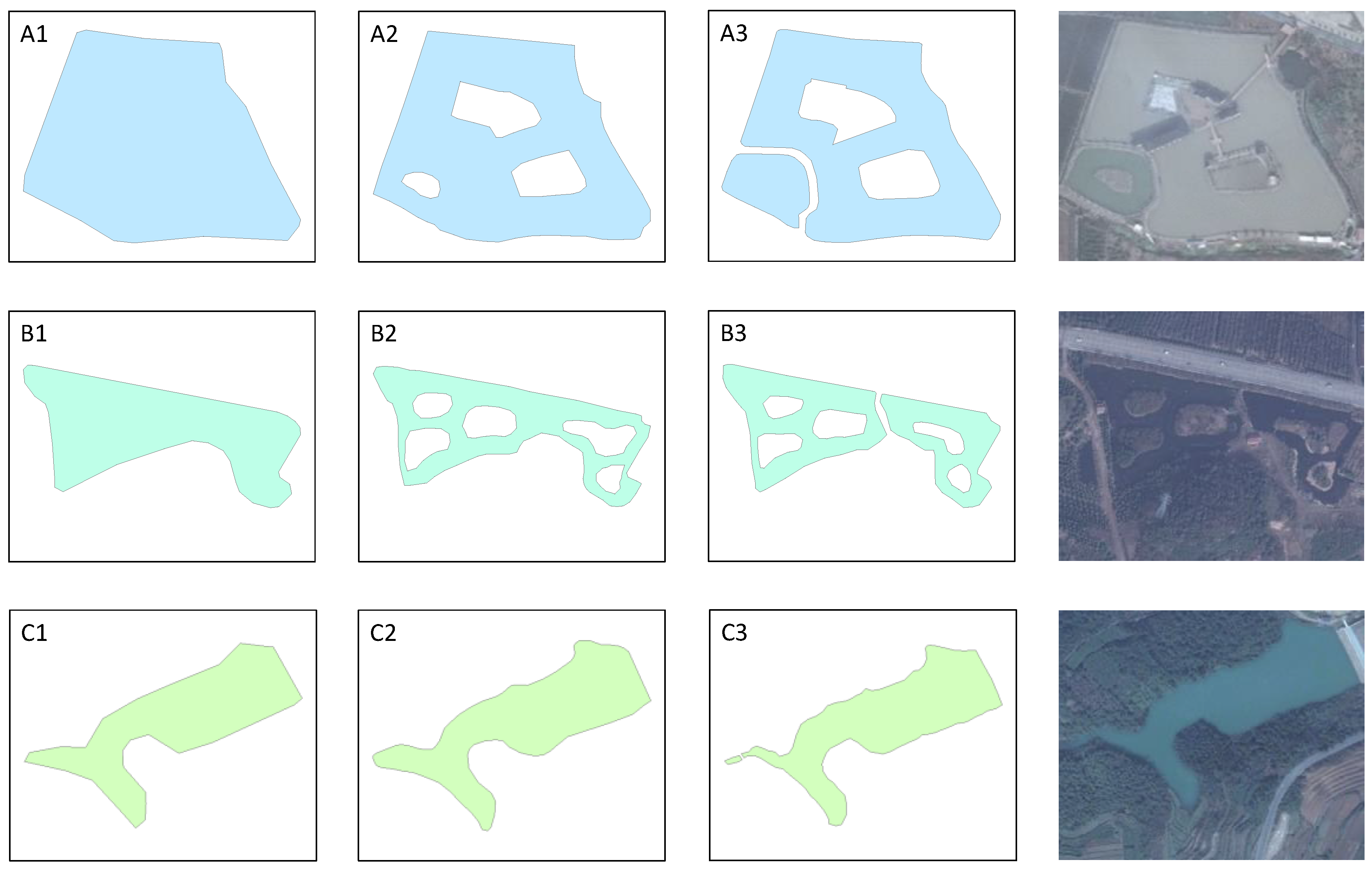
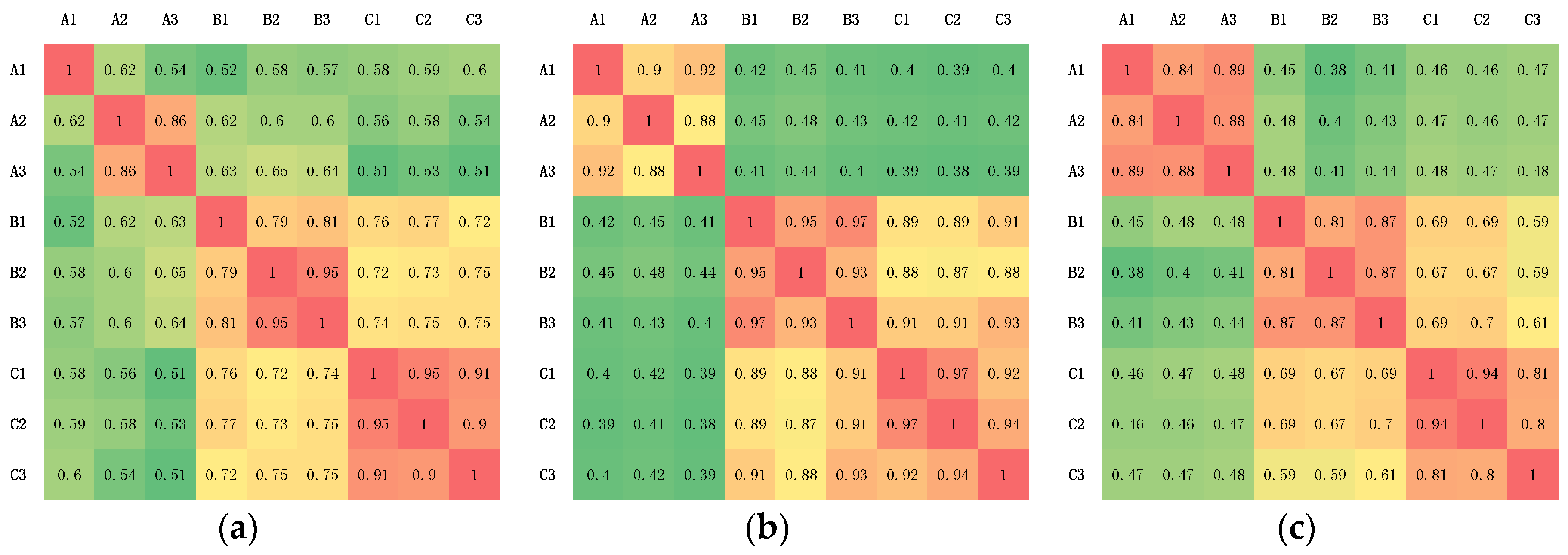
We choose three different lakes as study of areal entities to calculate the similarity between polygons to validate our shape description model. Each lake is represented by three different polygons at multiscales. Thus, we can get nine polygons as shown in Figure 11. The last column in Figure 11 are images of the three lakes on Bing maps. We found that the lake can be represented by either simple polygon or holed polygon or multipolygon. This multi-interpretation brings challenge to the similarity measurement between areal entities. Polygons representing the same lake are similar in boundaries. However, multipolygons have several disjoint boundaries and it is difficult to compare them with other types of polygons. Convex hull can extract boundary information of multipolygons. Moreover, convex hulls of different types of polygons can be comparable. However, different areal entities may also have similar convex hulls such as lake B and C.
In this paper, we take two similarity measurements as the comparison methods of ours. In the first comparison method, we use Zernike moments proposed in reference [21] to measure similarities of areal entities. Due to the complicated form of Zernike moments, it is difficult to derive calculation method for vector polygons. Thus, we transform vector polygons into binary images and then calculate the lower order Zernike moments of binary images. The similarity between polygons can be represented by the similarity between binary images. Transformation from vector polygons to images may introduce bias to the similarity measurement. In order to reduce the bias, we set the spatial resolution of images to 0.1 meter and also set the positional accuracy of vector polygons to 0.1 meter. In the second comparison method, we used Fourier descriptors proposed in reference [17] to measure similarities of convex hull. Thus, the similarity between areal entities can be represented by the similarity between convex hulls. Then, we measured the similarities between nine polygons in Figure 11 and we could get similarity matrix for different similarity measurements (Figure 12). The value of cells in the matrices are similarities between polygons. Values on the diagonal line of matrices are 1 because they are similarities between the same polygons. In order to make comparisons visually, we mapped the value of similarity to the color band. The red cells mean they have higher similarity value while the green cells mean they have lower similarity value. It can be observed that Zernike moments similarity measurement can distinguish different shapes while it isolates A1 from A2 and A3, and isolates B1 from B2 and B3. Fourier descriptors of convex hull can distinguish polygons of lake A while mix polygons of lake B and C. Our method can distinguish different lakes well. All of three methods can measure similarity between different types of polygons. However, shape similarity between areal entities is different from that of polygons. Because map generalization affects shape representation of areal entities. Different polygons representing the same areal entity are only similar in rough boundary features. The same areal entities with similar boundary features but different internal structures may differ in shape. Thus, Zernike moments isolate simple polygons from holed polyogns and multipolygons although they represent the same areal entities. On the other hand, different areal entities may have similar boundary features. Therefore, Fourier descriptors of convex hull mix different areal entities that have similar convex hull. Our method uses convex hull to identify same areal entities and uses moment invariants to distinguish different areal entities that have similar convex hull. It combines similar characteristics of convex hull and difference in shape features of polygons. Besides, we transform vector polygons into high resolution binary images to reduce bias in the method of Zernike moments. However, this transformation may increase the calculation of Zernike moments. Our method calculates moment invariants directly and has no bias. Fourier descriptors of convex hull can be calculated simply and directly. However, they are not invariant to scaling.
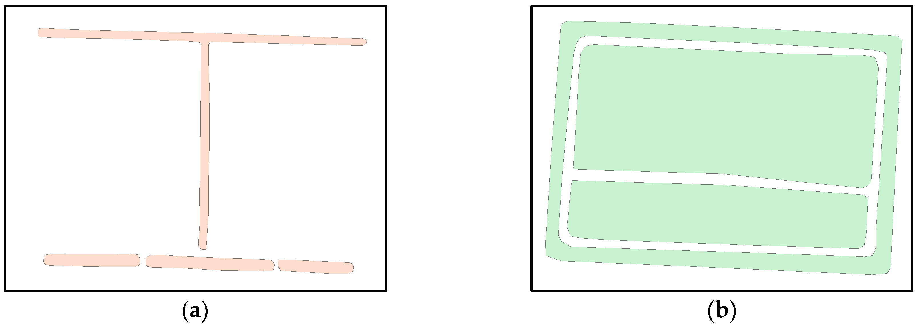
5.3. Experiment of Matching
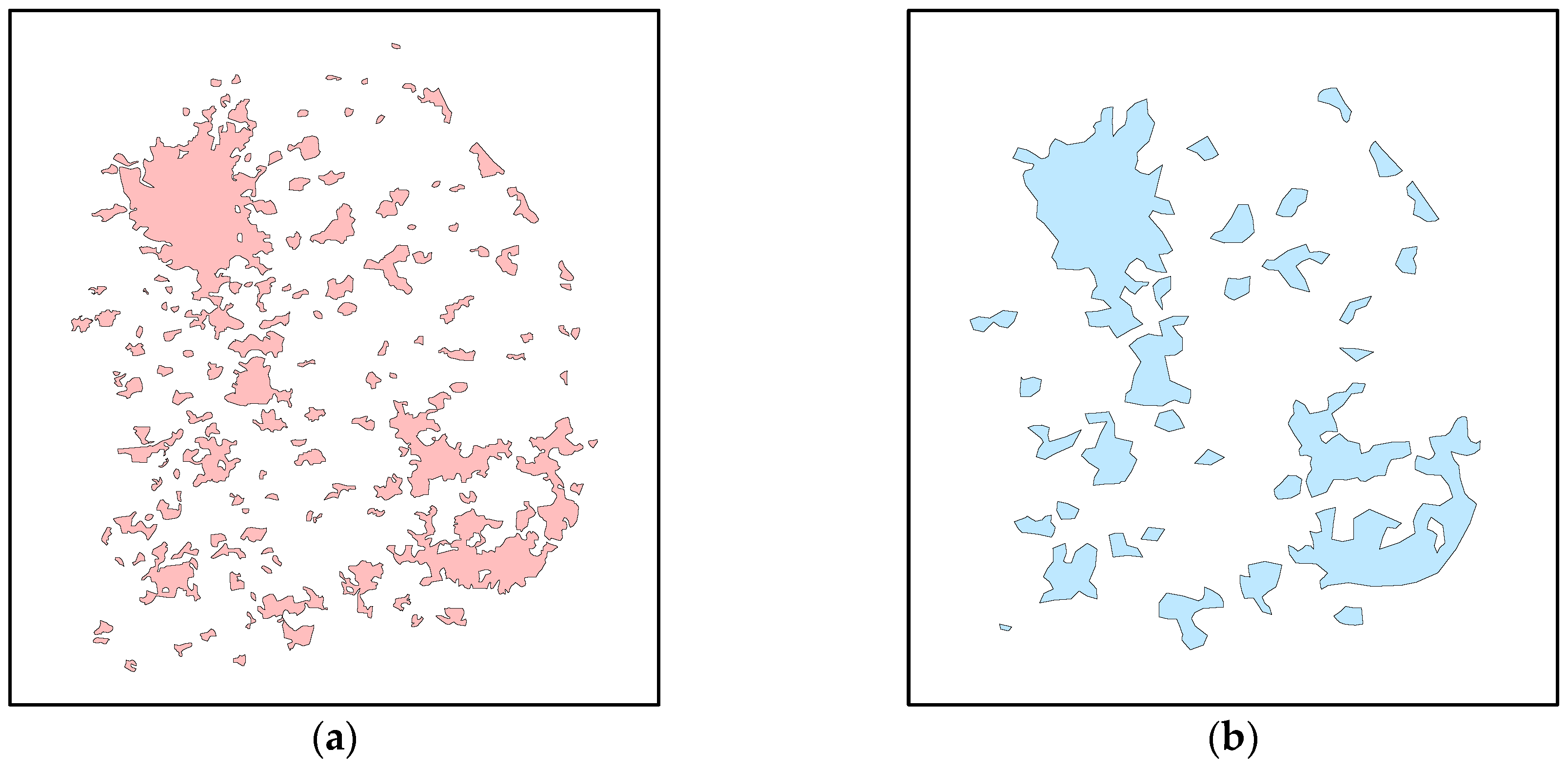
We also applied our method to the matching of two urban area datasets in different scales (Figure 13). The matching strategy we used is a similarity-based method proposed by Tang et al. [11]. In addition, we took their similarity measurement as a comparison method of ours. Then, we used precision, recall, and F1-score that are defined in the paper [10] to assess the matching results. The matching results of two methods are shown in Table 3. The method of Tang et al. uses a shape description function to measure shape similarity. It describes the shape by contour of polygons and can only be applied to simple polygons. Thus, there are many unmatched pairs in their method. Our method can be applied to simple polygons, holed polygons and multipolygons. Therefore, it can be found that our method has a higher precision and recall. Besides, the shape description function needs to match starting points on the boundary of polygons firstly. Mismatching of starting points will affect shape similarity between polygons. Our method is independent on starting points through fast Fourier transform and more robust to noise.
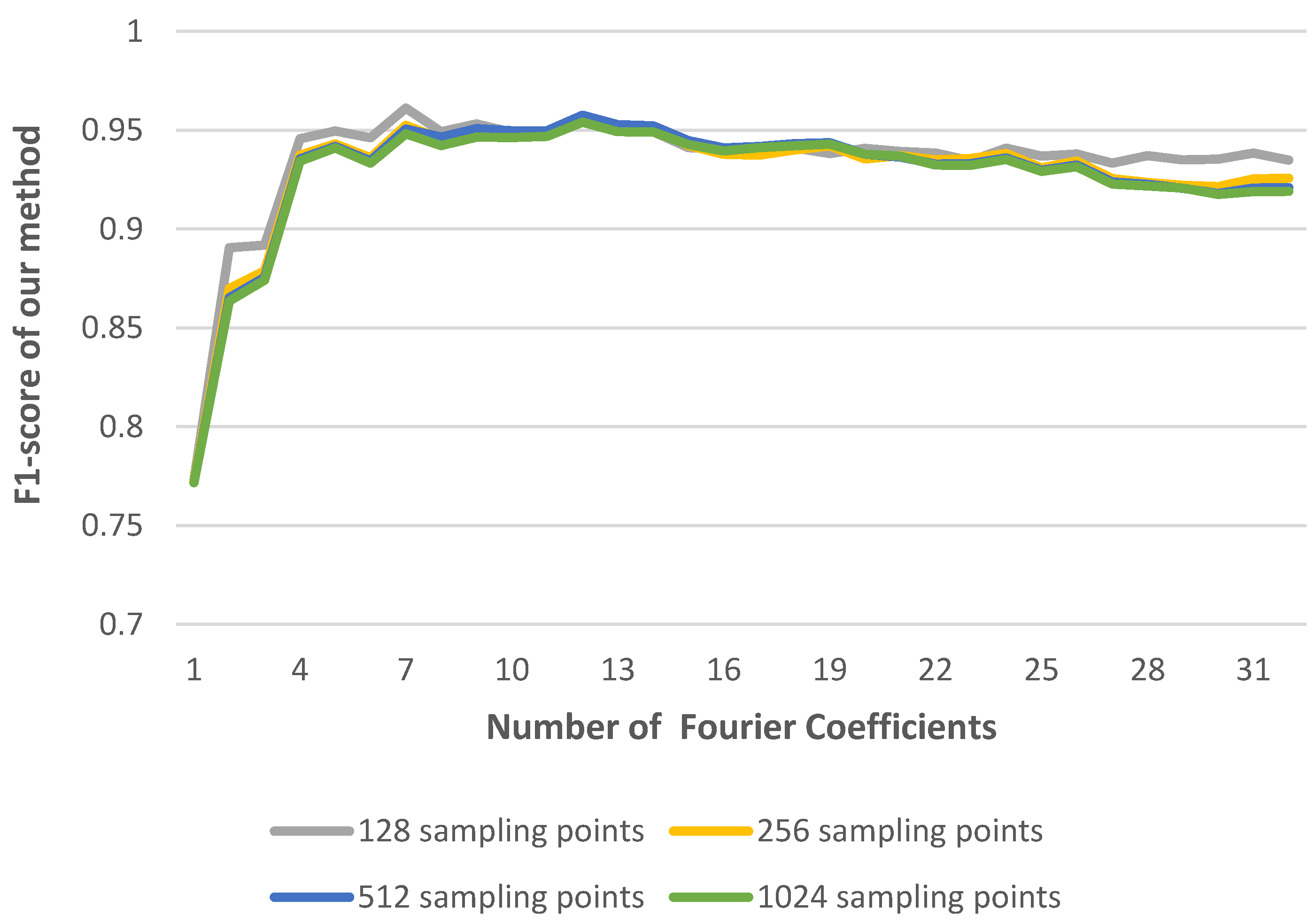
There are two parameters in our shape similarity measurement. They are the number of sampling points of convex hull and the number of Fourier coefficients. A large number of sampling points can describe the convex hull accurately, but require more calculations. Additionally, noise components may be located in the higher frequencies, it is necessary to select the first k Fourier coefficients to measure the similarity. Thus, we calculate F1-score of our method under different value of parameters (Figure 14). It can be observed that the number of sampling points larger than 256 and the number of Fourier coefficients larger than seven can reach a stable value of F1-score. Considering the computational efficiency, we chose 256 sampling points and top seven Fourier coefficients in our method.
6. Conclusions
Matching of areal entities is a key problem in geospatial data processing. Shape is one of the basic features for the matching of areal entities. Based on the idea of describing shape feature by moment invariants, this paper proposes an approach to describe shape feature by combining convex hull with moment invariants. The method uses convex hull to calculate local moment invariants of a polygon and then constructs convex hull moment invariant curves to describe the shape of polygon. By fast Fourier transform, the shape descriptor of the polygon can be extracted from the curves and can be used to measure shape similarity between different polygons. The experiments indicate that our shape descriptor is invariant under the transformation of translation, rotation, and scaling. In addition, our shape similarity measurement takes full advantage of moment invariants and convex hull. It can distinguish different areal entities even though they are represented by different kinds of polygons and vary in shape. Moreover, the method is applicable to the matching of areal entities in multi-scales.
Although the method is believed to be useful, there are issues for further investigation. The proposed method requires some parameters. We need to test a range of values to find the optimal parameters, which is time consuming. In addition, multi-representation of areal entities is a complicated problem. Areal entities represented by different polygons are not only similar in shape but also similar in direction, position, size, semantics, and topological relationships. In future research, we will investigate the comprehensive similarity measurement model that combines geometric features, topological features and semantic features for areal entities.
Author Contributions
Z.F. and L.F. conceived and designed the experiments; Z.Y. and K.Z. performed the experiments; L.F. collected the data and wrote the paper.
Conflicts of Interest
The authors declare no conflict of interest. The funding sponsors had no role in the design of the study; in the collection, analyses, or interpretation of data; in the writing of the manuscript, and in the decision to publish the results.
Appendix A
Geometric moments of a simple polygon are two-dimensional integral. However, vector polygons only have contour information. According to the Green’s formula, we can transform the double integral into a line integral along the boundary of a polygon.
Green’s formula:The closed area D is surrounded by a piecewise smooth curve L. P(x,y) and Q(x,y) are functions that have first-order continuous partial derivatives on D, then:
where L is the positive boundary curve of D.
Substituting into the Green’s formula, we can get the equation as follows:
For a simple polygon S, if L is the positive boundary curve of S, dividing L into line segments that are connected end to end with each other. It can be represented as , where Li represents the line segment connected by (xi,yi) and (xi+1,yi+1). Combining Equation (A2), we can get the (p + q)th order geometric moment of S:
where is the contour integral of , .
When Li is not perpendicular to the x-axis, it can be represented as follows:
where , .
Substituting Equation (A4) into and applying Binomial Theorem, we can get the equation as follows:
When Li is perpendicular to the x-axis, can be calculated directly:
For a holed polygon , we can also use the Green’s formula to convert integral of the holed polygon region into line integral of rings:
For a multipolygon , we can easily derive the equation of line integral form as follows:
each summation in Equations (A7) and (A8) can be calculated by the method of a simple polygon.
References
- Walter, V.; Fritsch, D. Matching spatial data sets: A statistical approach. Int. J. Geogr. Inf. Sci. 1999, 13, 445–473. [Google Scholar] [CrossRef]
- Cobb, M.A.; Chung, M.J.; Foley, H., III; Petry, F.E.; Shaw, K.B.; Miller, H.V. A rule-based approach for the conflation of attributed vector data. GeoInformatica 1998, 2, 7–35. [Google Scholar] [CrossRef]
- Saalfeld, A. Conflation automated map compilation. Int. J. Geogr. Inf. Syst. 1988, 2, 217–228. [Google Scholar] [CrossRef]
- Al-Bakri, M.; Fairbairn, D. Assessing similarity matching for possible integration of feature classifications of geospatial data from official and informal sources. Int. J. Geogr. Inf. Sci. 2012, 26, 1437–1456. [Google Scholar] [CrossRef]
- Fan, H.; Zipf, A.; Fu, Q.; Neis, P. Quality assessment for building footprints data on Open Street Map. Int. J. Geogr. Inf. Sci. 2014, 28, 700–719. [Google Scholar] [CrossRef]
- Zhao, Y.J.; Zhou, X.G. Version similarity-based model for volunteers’ reputation of volunteered geographic information: A case study of polygon. Acta Geod. Cartogr. Sin. 2015, 44, 578–584. [Google Scholar]
- Koukoletsos, T.; Haklay, M.; Ellul, C. Assessing Data Completeness of VGI through an Automated Matching Procedure for Linear Data. Trans. Gis 2012, 16, 477–498. [Google Scholar] [CrossRef]
- Kim, J.O.; Yu, K.; Heo, J.; Lee, W.H. A new method for matching objects in two different geospatial datasets based on the geographic context. Comput. Geosci. 2010, 36, 1115–1122. [Google Scholar] [CrossRef]
- Zhang, Q.P.; Li, D.R.; Gong, J.Y. Map conflation. Bull. Surv. Mapp. 2001, 7, 6–8. [Google Scholar]
- Xavier, E.; Ariza-López, F.J.; Urena-Camara, M.A. A survey of measures and methods for matching geospatial vector datasets. ACM Comput. Surv. 2016, 49, 39. [Google Scholar] [CrossRef]
- Tang, W.; Hao, Y.; Zhao, Y.; Ning, L. Research on areal feature matching algorithm based on spatial similarity. In Proceedings of the Control and Decision Conference, Yantai, China, 2–4 July 2008; pp. 3326–3330. [Google Scholar]
- Yang, M.; Kpalma, K.; Ronsin, J. A Survey of Shape Feature Extraction Techniques. Pattern Recognit. 2010, 1, 43–90. [Google Scholar]
- Fu, Z.L.; Shao, S.W.; Tong, C.Y. Multi-scale area entity shape matching based on tangent space. Comput. Eng. 2010, 17, 74. [Google Scholar]
- An, X.; Sun, Q.; Xiao, Q.; Yan, W. A shape multilevel description method and application in measuring geometry similarity of multi-scale spatial data. Acta Geod. Cartogr. Sin. 2011, 40, 495–508. [Google Scholar]
- Chen, Z.; Qin, M.; Wu, L.; Xie, Z. Establishment of the comprehensive shape similarity model for complex polygon entity by using bending mutilevel chord complex function. Acta Geod. Cartogr. Sin. 2016, 45, 224–232. [Google Scholar]
- Belongie, S.; Malik, J.; Puzicha, J. Shape context: A new descriptor for shape matching and object recognition. Adv. Neural Inf. Process. Syst. 2000, 831–837. [Google Scholar]
- Zhang, D.; Lu, G. A Comparative Study on Shape Retrieval Using Fourier Descriptors with Different Shape Signatures. In Proceedings of the International Conference on Intelligent Multimedia and Distance Education (ICIMADE01), Fargo, ND, USA, 1–3 June 2001; pp. 1–9. [Google Scholar]
- Xu, Y.; Xie, Z.; Chen, Z.; Wu, L. Shape similarity measurement model for holed polygons based on position graphs and Fourier descriptors. Int. J. Geogr. Inf. Sci. 2017, 31, 253–279. [Google Scholar] [CrossRef]
- Schneider, M.; Behr, T. Topological relationships between complex spatial objects. ACM Trans. Datab. Syst. 2006, 31, 39–81. [Google Scholar] [CrossRef]
- Chen, Z.; Zhu, R.; Xie, Z.; Wu, L. Hierarchical Model for the Similarity Measurement of a Complex Holed-Region Entity Scene. ISPRS Int. J. Geo Inf. 2017, 6, 388. [Google Scholar] [CrossRef]
- Kim, W.Y.; Kim, Y.S. A region-based shape descriptor using Zernike moments. Signal Process. Image Commun. 2000, 16, 95–102. [Google Scholar] [CrossRef]
- Premaratne, P.; Premaratne, M. Image matching using moment invariants. Neurocomputing 2014, 137, 65–70. [Google Scholar] [CrossRef]
- Zhang, D.; Lu, G. Review of shape representation and description techniques. Pattern Recognit. 2004, 37, 1–19. [Google Scholar] [CrossRef]
- Chen, Z.; Feng, Q.; Wu, X. Representation model of topological relations between complex planar objects. Acta Geod. Cartogr. Sin. 2015, 44, 438–444. [Google Scholar]
- Clementini, E.; di Felice, P. A model for representing topological relationships between complex geometric features in spatial databases. Inf. Sci. 1996, 90, 121–136. [Google Scholar] [CrossRef]
- Ai, T.; Li, Z.; Liu, Y. Progressive Transmission of Vector Data Based on Changes Accumulation Model. Dev. Spat. Data Handl. 2005. [Google Scholar] [CrossRef]
- Lu, G.; Sajjanhar, A. Region-based shape representation and similarity measure suitable for content-based image retrieval. Multimed. Syst. 1999, 7, 165–174. [Google Scholar] [CrossRef]
- Kim, H.K.; Kim, J.D. Region-based shape descriptor invariant to rotation, scale and translation. Signal Process. Image Commun. 2000, 16, 87–93. [Google Scholar] [CrossRef]
- Karakasis, E.G.; Amanatiadis, A.; Gasteratos, A.; Chatzichristofis, S.A. Image moment invariants as local features for content based image retrieval using the Bag-of-Visual-Words model. Pattern Recognit. Lett. 2015, 55, 22–27. [Google Scholar] [CrossRef]
- Hu, M.K. Visual pattern recognition by moment invariants. IRE Trans. Inf. Theory 1962, 8, 179–187. [Google Scholar]
- Jiang, X.Y.; Bunke, H. Simple and fast computation of moments. Pattern Recognit. 1991, 24, 801–806. [Google Scholar] [CrossRef]
- Cai, H.; Zhu, F. Shape Matching Method Based on Convex Hull and Multiscale Integral Features under Affine Transformation. J. Comput. Aided Des. Comput. Gr. 2017, 29, 269–278. [Google Scholar]
- Zhao, D.B.; Tian, H.E.; Zhang, K. Shape Contour Description and Matching Method Based on Complex Moments. J. Sichuan Univ. 2011, 43, 109–115. (In Chinese) [Google Scholar]
Figure 1.
Qinghai Lake in multiple representations (a) Simple polygon, (b) holed polygon, (c) multipolygon; and (d) Bing maps.
Figure 1.
Qinghai Lake in multiple representations (a) Simple polygon, (b) holed polygon, (c) multipolygon; and (d) Bing maps.


Figure 2.
Same lakes at different scales and convex hulls of the lakes: (A) Polygon A is the lake in scale of 1:10,000, (B) polygon B is the lake in scale of 1:50,000, (C) polygon C is convex hull of polygon A; and (D) polygon D is convex hull of polygon B.
Figure 2.
Same lakes at different scales and convex hulls of the lakes: (A) Polygon A is the lake in scale of 1:10,000, (B) polygon B is the lake in scale of 1:50,000, (C) polygon C is convex hull of polygon A; and (D) polygon D is convex hull of polygon B.

Figure 3.
Different areal entities with similar convex hulls: (a) the canals and (b) the canal with two pools.
Figure 3.
Different areal entities with similar convex hulls: (a) the canals and (b) the canal with two pools.

Figure 4.
Transformation method of center moments and local moments: (a) Original position of the polygon, (b) moving the origin of coordinates to the centroid of the polygon; and (c) the red polyline is the boundary of convex hull, moving the origin of coordinates to the point on the boundary of convex hull.

Figure 5.
Convex hull moment invariant curves of the polygon in Figure 4: (a) Convex hull moment invariant curves and (b) centroid distance of convex hull vertices.
Figure 5.
Convex hull moment invariant curves of the polygon in Figure 4: (a) Convex hull moment invariant curves and (b) centroid distance of convex hull vertices.

Figure 6.
The lake at different scales: (a) the lake in scale of 1:10,000 and (b) the lake in scale of 1:50,000.
Figure 6.
The lake at different scales: (a) the lake in scale of 1:10,000 and (b) the lake in scale of 1:50,000.

Figure 7.
Convex hull moment invariant curves of the lake in scale of 1:10,000.

Figure 8.
Convex hull moment invariant curves of the lake in scale of 1:50,000.

Figure 9.
Shape descriptor of lakes in Figure 4: (a) Shape descriptor of the lake in scale of 1:10,000 and (b) shape descriptor of the lake in scale of 1:50,000.
Figure 9.
Shape descriptor of lakes in Figure 4: (a) Shape descriptor of the lake in scale of 1:10,000 and (b) shape descriptor of the lake in scale of 1:50,000.

Figure 10.
Three countries represented by different types of polygons: (a) Switzerland, (b) South Africa, (c) Japan, (d) Switzerland after transformation, (e) South Africa after transformation; and (f) Japan after transformation.
Figure 10.
Three countries represented by different types of polygons: (a) Switzerland, (b) South Africa, (c) Japan, (d) Switzerland after transformation, (e) South Africa after transformation; and (f) Japan after transformation.

Figure 11.
Three different lakes represented by nine polygons at multiscales.

Figure 12.
Shape similarity results of three different lakes: (a) shape similarity matrix by Zernike moments, (b) shape similarity matrix by Fourier descriptors of convex hull; and (c) shape similarity matrix by our method.
Figure 12.
Shape similarity results of three different lakes: (a) shape similarity matrix by Zernike moments, (b) shape similarity matrix by Fourier descriptors of convex hull; and (c) shape similarity matrix by our method.

Figure 13.
Urban area datasets in different scales: (a) dataset A in scale of 1:100,000 and (b) dataset B in scale of 1:500,000.
Figure 13.
Urban area datasets in different scales: (a) dataset A in scale of 1:100,000 and (b) dataset B in scale of 1:500,000.

Figure 14.
F1-score of our method under different value of parameters.


Table 1.
Hu moment invariants of six polygons.
| C1 | C2 | C3 | C4 | C5 | C6 | C7 | |
|---|---|---|---|---|---|---|---|
| a | 2.462 × 10⁻¹ | 3.001 × 10⁻² | 5.989 × 10⁻⁴ | 7.151 × 10⁻⁵ | −1.355 × 10⁻⁹ | −6.198 × 10⁻⁶ | 1.474 × 10⁻⁸ |
| b | 2.132 × 10⁻¹ | 1.419 × 10⁻² | 4.689 × 10⁻⁴ | 5.192 × 10⁻⁵ | 9.138 × 10⁻¹⁰ | −1.832 × 10⁻⁶ | −8.048 × 10⁻⁹ |
| c | 8.181 × 10⁻¹ | 5.197 × 10⁻¹ | 1.008 × 10⁻¹ | 1.375 × 10⁻² | −1.481 × 10⁻⁴ | −5.535 × 10⁻³ | 4.903 × 10⁻⁴ |
| d | 2.462 × 10⁻¹ | 3.001 × 10⁻² | 5.989 × 10⁻⁴ | 7.151 × 10⁻⁵ | −1.355 × 10⁻⁹ | −6.198 × 10⁻⁶ | 1.474 × 10⁻⁸ |
| e | 2.132 × 10⁻¹ | 1.419 × 10⁻² | 4.689 × 10⁻⁴ | 5.191 × 10⁻⁵ | 9.125 × 10⁻¹⁰ | −1.833 × 10⁻⁶ | −8.048 × 10⁻⁹ |
| f | 8.181 × 10⁻¹ | 5.197 × 10⁻¹ | 1.008 × 10⁻¹ | 1.376 × 10⁻² | −1.481 × 10⁻⁴ | −5.536 × 10⁻³ | 4.903 × 10⁻⁴ |
Table 2.
Shape descriptor of six polygons.
| C1F1 | C2F1 | C3F1 | C4F1 | C5F1 | C6F1 | C7F1 | C1F2 | C2F2 | C3F2 | C4F2 | C5F2 | C6F2 | C7F2 | |
|---|---|---|---|---|---|---|---|---|---|---|---|---|---|---|
| a | 9.89 × 101 | 6.36 × 101 | 9.17 × 101 | 1.20 × 10² | 2.13 × 10² | 1.16 × 10² | 2.27 × 10⁻² | 2.44 × 100 | 2.63 × 100 | 3.11 × 100 | 5.93 × 100 | 1.46 × 101 | 7.08 × 100 | 2.31 × 100 |
| b | 8.32 × 101 | 3.39 × 101 | 3.15 × 101 | 5.42 × 101 | 2.76 × 101 | 3.37 × 101 | 1.78 × 10⁻¹ | 3.48 × 100 | 1.79 × 100 | 4.10 × 10⁻¹ | 3.62 × 100 | 1.92 × 100 | 2.35 × 100 | 6.25 × 10⁻¹ |
| c | 3.52 × 10² | 1.15 × 10³ | 7.69 × 10³ | 8.27 × 10³ | 1.85 × 10⁶ | 4.14 × 10⁴ | 1.20 × 10³ | 8.91 × 101 | 6.53 × 10² | 5.31 × 10³ | 5.60 × 10³ | 1.72 × 10⁶ | 3.38 × 10⁴ | 1.52 × 10³ |
| d | 9.89 × 101 | 6.36 × 101 | 9.17 × 101 | 1.20 × 10² | 2.14 × 10² | 1.16 × 10² | 2.40 × 10⁻² | 2.44 × 100 | 2.63 × 100 | 3.09 × 100 | 5.92 × 100 | 1.46 × 101 | 7.07 × 100 | 2.31 × 100 |
| e | 8.32 × 101 | 3.39 × 101 | 3.15 × 101 | 5.42 × 101 | 2.76 × 101 | 3.37 × 101 | 1.77 × 10⁻¹ | 3.48 × 100 | 1.79 × 100 | 4.19 × 10⁻¹ | 3.62 × 100 | 1.94 × 100 | 2.36 × 100 | 6.26 × 10⁻¹ |
| f | 3.52 × 10² | 1.16 × 10³ | 7.69 × 10³ | 8.28 × 10³ | 1.86 × 10⁶ | 4.15 × 10⁴ | 1.21 × 10³ | 8.91 × 101 | 6.53 × 10² | 5.31 × 10³ | 5.61 × 10³ | 1.72 × 10⁶ | 3.39 × 10⁴ | 1.53 × 10³ |
Table 3.
Matching result for the methods.
| Method Described in | Correct | Wrong | Unmatch | Precision | Recall | F1-Score |
|---|---|---|---|---|---|---|
| Tang et al. [11] | 21 | 1 | 11 | 95.45% | 65.63% | 77.78% |
| Ours | 30 | 1 | 2 | 96.77% | 93.75% | 95.24% |
© 2018 by the authors. Licensee MDPI, Basel, Switzerland. This article is an open access article distributed under the terms and conditions of the Creative Commons Attribution (CC BY) license (http://creativecommons.org/licenses/by/4.0/).
Share and Cite
MDPI and ACS Style
Fu, Z.; Fan, L.; Yu, Z.; Zhou, K. A Moment-Based Shape Similarity Measurement for Areal Entities in Geographical Vector Data. ISPRS Int. J. Geo-Inf. 2018, 7, 208. https://doi.org/10.3390/ijgi7060208
AMA Style
Fu Z, Fan L, Yu Z, Zhou K. A Moment-Based Shape Similarity Measurement for Areal Entities in Geographical Vector Data. ISPRS International Journal of Geo-Information. 2018; 7(6):208. https://doi.org/10.3390/ijgi7060208
Chicago/Turabian StyleFu, Zhongliang, Liang Fan, Zhiqiang Yu, and Kaichun Zhou. 2018. "A Moment-Based Shape Similarity Measurement for Areal Entities in Geographical Vector Data" ISPRS International Journal of Geo-Information 7, no. 6: 208. https://doi.org/10.3390/ijgi7060208
Note that from the first issue of 2016, this journal uses article numbers instead of page numbers. See further details here.