Article

Trend Analysis of Relationship between Primary Productivity, Precipitation and Temperature in Inner Mongolia

1
Institute for Geospatial Research and Education, Eastern Michigan University, Ypsilanti, MI 48197, USA
2
School of Geomatics, Anhui University of Science and Technology, 168 Taifeng Ave., Huainan, China
3
Institute of Botany, Chinese Academy of Sciences, Beijing 100093, China
4
School of Mining and Geomatics, Hebei University of Engineering, 199 South Guangming St., Handan, China
5
Department of Geography, University of Georgia, 210 Field St #204, Athens, GA 30602, USA
*
Author to whom correspondence should be addressed.
ISPRS Int. J. Geo-Inf. 2018, 7(6), 214; https://doi.org/10.3390/ijgi7060214
Submission received: 13 March 2018 / Revised: 15 May 2018 / Accepted: 27 May 2018 / Published: 5 June 2018

Abstract

:
This study mainly examined the relationships among primary productivity, precipitation and temperature by identifying trends of change embedded in time-series data. The paper also explores spatial variations of the relationship over four types of vegetation and across two precipitation zones in Inner Mongolia, China. Traditional analysis of vegetation response to climate change uses minimum, maximum, average or cumulative measurements; focuses on a whole region instead of fine-scale regional or ecological variations; or adopts generic analysis techniques. We innovatively integrate Empirical Mode Decomposition (EMD) and Redundancy Analysis (RDA) to overcome the weakness of traditional approaches. The EMD filtered trend surfaces reveal clear patterns of Enhanced Vegetation Index (EVI), precipitation, and temperature changes in both time and space. The filtered data decrease noises and cyclic fluctuations in the original data and are more suitable for examining linear relationship than the original data. RDA is further applied to reveal partial effect of precipitation and temperature, and their joint effect on primary productivity. The main findings are as follows: (1) We need to examine relationships between the trends of change of the variables of interest when investigating long-term relationships among them. (2) Long-term trend of change of precipitation or temperature can become a critical factor influencing primary productivity depending on local environments. (3) Synchronization (joint effect) of precipitation and temperature in growing season is critically important to primary productivity in the study area. (4) Partial and joint effects of precipitation and temperature on primary productivity vary over different precipitation zones and different types of vegetation. The method developed in this paper is applicable to ecosystem research in other regions.

1. Introduction

Vegetation is one of the most important components of an ecosystem and is affected by interaction between terrestrial and atmospheric systems through carbon and hydrologic cycles [1,2]. Vegetation growth is very sensitive to meteorological condition as well as climate change [3,4,5,6]. Climate change is commonly recognized as one of the most important drivers that are affecting plant ecosystems [7]. Drying and warming climate usually decreases vegetation productivity [8,9], while wet climate usually facilitates plant growth [3,10].
Climate change has been an ongoing process since geological time. Climate change is marked with variation either in temperature or in precipitation, or in both [11]. Rising temperature and decreasing precipitation were the primary causes of grassland degradation in Inner Mongolia, China [9,12,13]. In addition, climate change has displayed significant spatial variations. Damsø and his colleagues [14] pointed out that climate change is more apparent or noticeable to humans in mountainous areas than in low and flat regions. Meteorological conditions vary locally due to different configurations of elevation, topography, landscape, vegetation cover, water body, dominant wind direction and human-made objects. Varied interactions between local terrestrial and atmospheric systems can have profound impacts on local meteorological conditions. Therefore, it is a norm that distinct regional patterns of climate change are observed [15]. Furthermore, it is recognized that different plant communities show varied responses to climate change [16]. Plant communities respond differently to short-term or long-term changes of precipitation and temperature [2,17]. Responses of plant communities to climate change display significant local and regional variations [13,18,19].
In ecological and geographical sciences, there is a long tradition to study spatial variability of climate change, its impact on vegetation growth and varied response of vegetation to climate change [20]. However, the studies of climate change and regional and local interactions between climate change and vegetation growth have faced many challenges. First, although it is relatively easy to find long records of climate change, it is difficult to find long time-series data about vegetation growth and evolution [9]. Second, both climate change and vegetation growth display distinctive seasonal and annual fluctuations as well as abrupt variations. Trends of long-term change are buried within these cyclical and abrupt changes. It is almost impossible to treat interactions between climate change and vegetation growth as linear. As a result, most current statistical analysis methods cannot be directly used to examine their interactions. Third, although it has long been assumed that vegetation growth has been primarily affected by both precipitation and temperature changes [3], it is hard to distinguish which meteorological factor (precipitation or temperature) has a stronger impact on vegetation growth. It is much more challenging to know under which local ecological environment a meteorological factor has the strongest effect on vegetation growth. Finally, current studies of vegetation growth and its response to climate change are often using time-averaged or cumulative data to develop ecological or environmental models. These models usually analyze minimum, average or maximum values of observations within a period of study. The temporal granite is too coarse to effectively separate long-term trends from cyclical fluctuations and abrupt changes or capture temporal dynamics or regional patterns of ecosystem change [13,21,22,23,24].
In this paper, we attempt to differentiate which meteorological factor (precipitation or temperature) has greater impact on primary productivity; to examine how precipitation and temperature affect primary productivity; and to determine whether the effect of precipitation and temperature on primary productivity varies over different precipitation zones and different types of vegetation. Since traditional analysis of vegetation response to climate change uses minimum, maximum, average or cumulative measurements, or focuses on a whole region instead of fine-scale regional or ecological variations, we innovatively integrate several analytical techniques in this paper to overcome the above challenges. As stated above, the overall trends of EVI, precipitation, and temperature are extracted via EMD and, then, redundancy analysis is integrated to examine partial and joint effects of precipitation and temperature on primary productivity at regional, local and plant community scales.

2. Data and Method

2.1. The Study Area

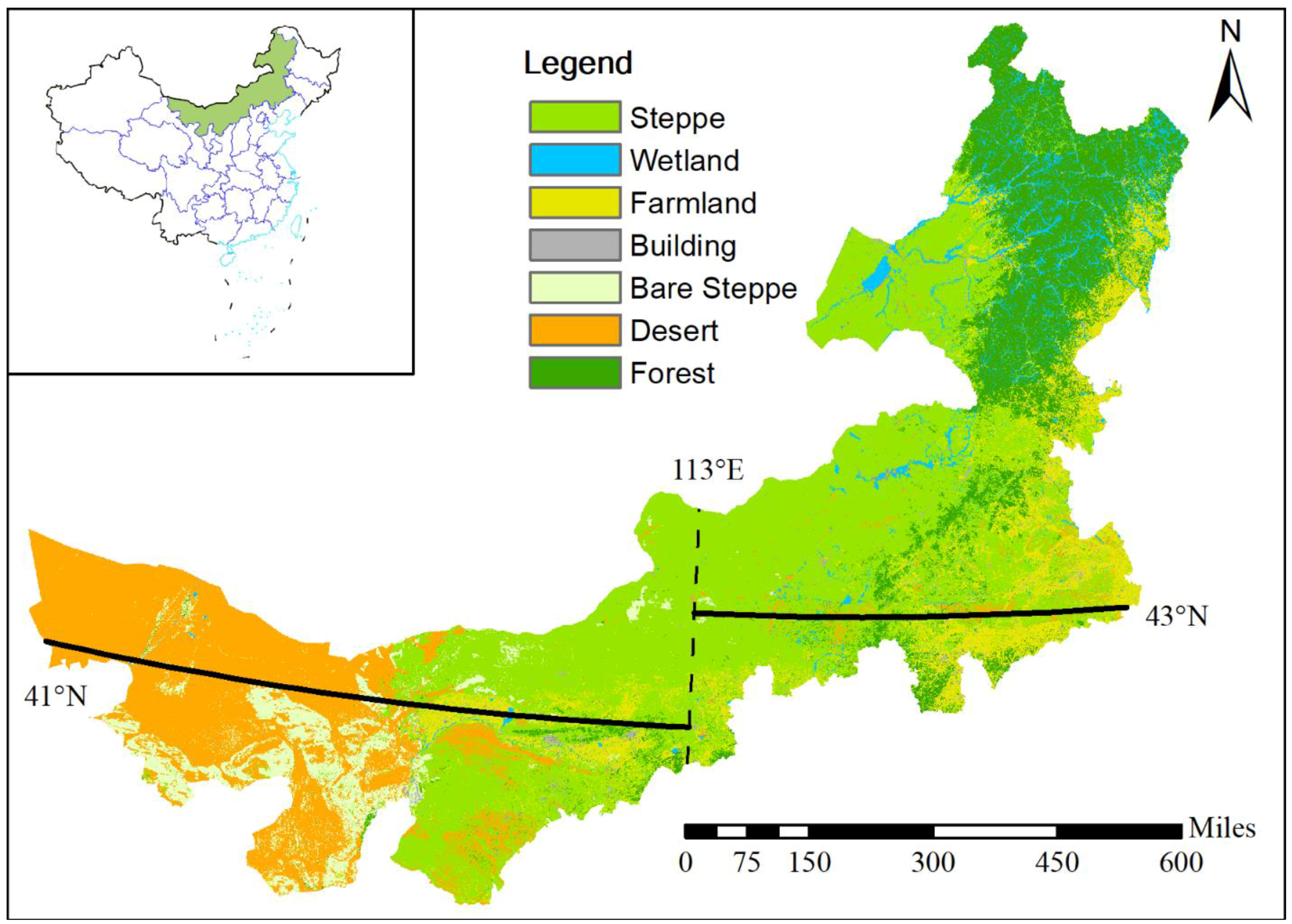
The Inner Mongolia Plateau (IMP) is chosen as the study area (Figure 1). IMP boasts the most important grassland resource in northern China [25]. IMP extends from 37.40° N to 53.38° N and from 97.2° E to 126.06° E, covering an area of 1.18 million square kilometers [3]. IMP has an annual precipitation 50–450 mm and an annual average temperature 1–10 °C. Both precipitation and temperature display a regional transition from semi-humid areas in east to semiarid and arid areas in west. Grassland degradation is a serious threat to sustainability of these ecosystems [26,27,28]. Northern China and, especially, Inner Mongolia Plateau have suffered severe ecological degradation in recent decades [29,30,31]. It is important for researchers, policy makers and resource managers to understand how each vegetation community responds to climate change. There are an increasing number of studies reported in current literature. Several examine status change of vegetation evolution [2,32]. Some investigate coupled impact of socioeconomic transformation and climate change on vegetation growth [9,13,33]. Few are about composition structure and its relationship with climate factors [15,34]. Most studies are focused on regional scale and interested in identifying regional patterns [2,35,36]. Little effort has been exerted to explore vegetation growth response to climate change among different plant communities over various precipitation zones [37,38].
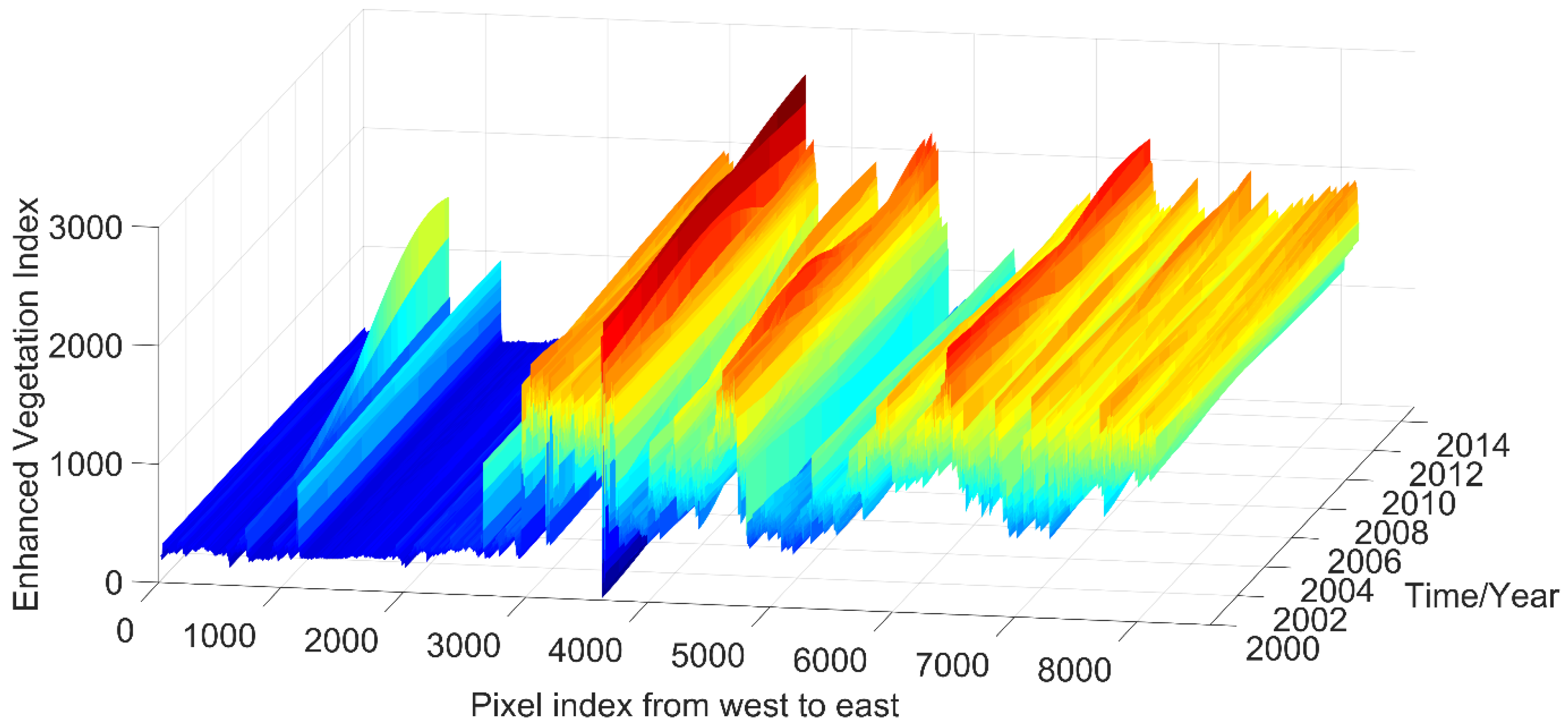
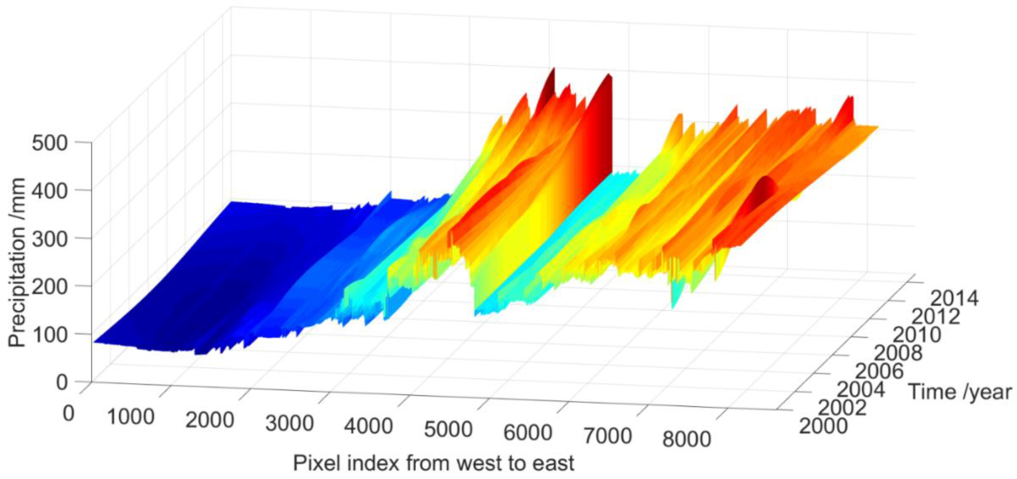
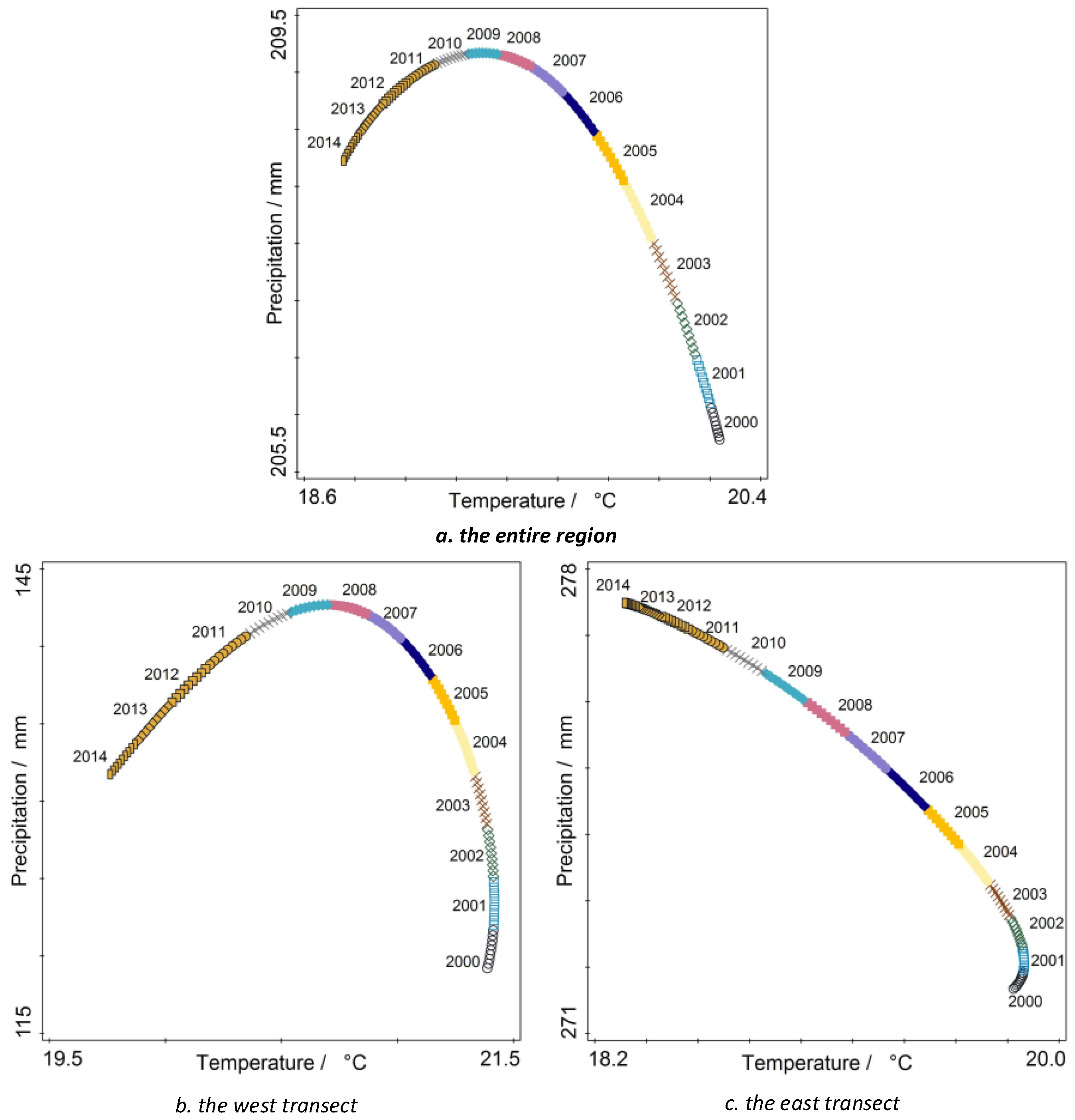
For the above reasons, we focused on revealing spatial and temporal change patterns of grassland communities over an east-to-west transection and how the changes are related to the fluctuations of precipitation and temperature at both regional and local scales. Therefore, we designed a horizontal transect extending from east to west across the entire study area. Due to the unique shape of the study area, we bisected the transect i at 113° E, which is an ideal position to separate the transect into two sections that cover the majorities of vegetation communities in the study area (Figure 1). In addition, we examined four major land covers and uses in the study area, typical steppe, bare steppe, desert and farmland.

2.2. The Data and Pre-Processing

The data used in this paper include three datasets: Modis EVI (enhanced vegetation index), meteorological observations (of precipitation and temperature), and IMP land cover map 2010. EVI was adopted as a proxy of the vegetation primary productivity instead of NDVI [35,39,40], since EVI overcomes the saturation and soil noise problems of NDVI by decreasing the atmospheric effect and reducing the canopy background [41]. The 16-day EVI data with 250 m spatial resolution for 2000–2014 were collected from MODIS 13Q1, which is available at https://lpdaac.usgs.gov/data_access/data_pool. Nine 16-day periods during the growing season each year (8 May to 28 September) were included in the analysis [
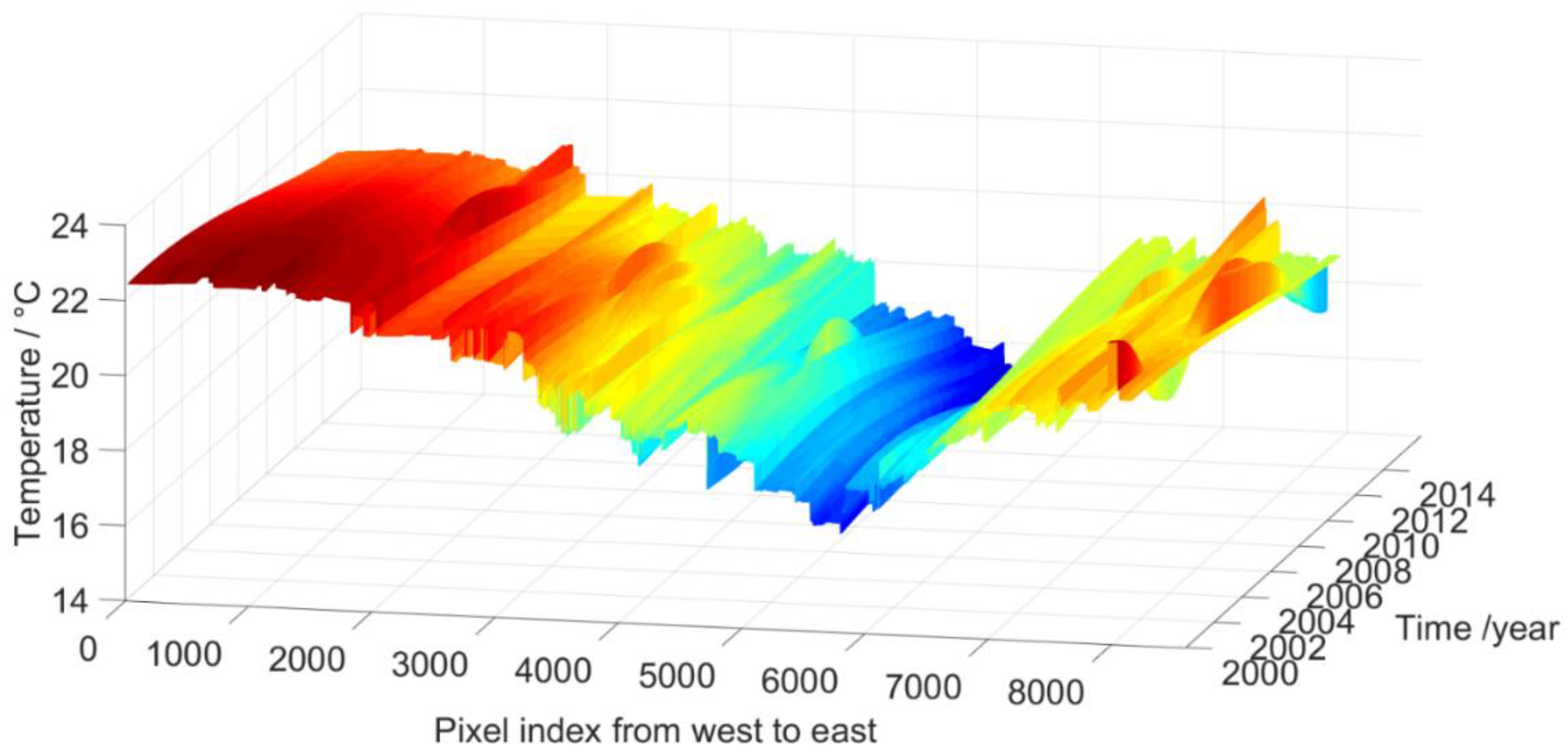
42] totally 135 periods (15 years × 9 periods). Further, the transects were clipped out in ArcGIS by two buffers with 1750 m (a length of 7 pixels) along 41° N and 43° N. This clipping process was also applied to the following two datasets.
Meteorological data were extracted from the China Meteorological Data Service Center (CMDC, 2013). There are 50 meteorological stations in the study area. Two meteorological factors, precipitation and temperature, were selected for the analysis. The original climate data were the daily record from 2000 to 2014. To be consistent with the EVI data, the accumulation of precipitation and the mean temperature for each of the nine 16-day periods during the growing season were calculated. These values at 50 stations were spatially interpolated as precipitation and temperature surfaces at 250 m resolution, respectively. The interpolations were processed using inverse distance weighting (IDW) method. Cross-validation was used to calibrate the best pair of interpolation parameters (power and radius) over the data of the nine periods of 2014 [43]. Forty stations were chosen as the training sample to execute IDW interpolation and ten were reserved as the validation sample. The root mean square error (RMSE) was used to judge the validation outcomes. The validation result showed that the RMSE of temperature between the estimated value and validation value was around 6% and the RMSE of precipitation was about 18%. Due to the dramatic spatial variation of precipitation in IMP [21,44,45], the RMSE of precipitation was much higher than the RMSE of temperature but was reasonably small.
The 2010 Inner Mongolia land cover classification map was provided by Institute of Remote Sensing and Digital Earth, China [9]. The map was made through interpreting the Landsat images along with ground reference points. The original spatial resolution of the product was 30 m. The vegetation map was resampled to 250 m so that it had the same resolution as EVI. In brief, EVI, precipitation, and temperature were pre-processed with the same spatial and temporal resolutions and each of them had a 135-period time series (2000–2014, with 9 periods per year in growing season).

2.3. The Analysis Method

We synthesized the integrated research method depicted in 
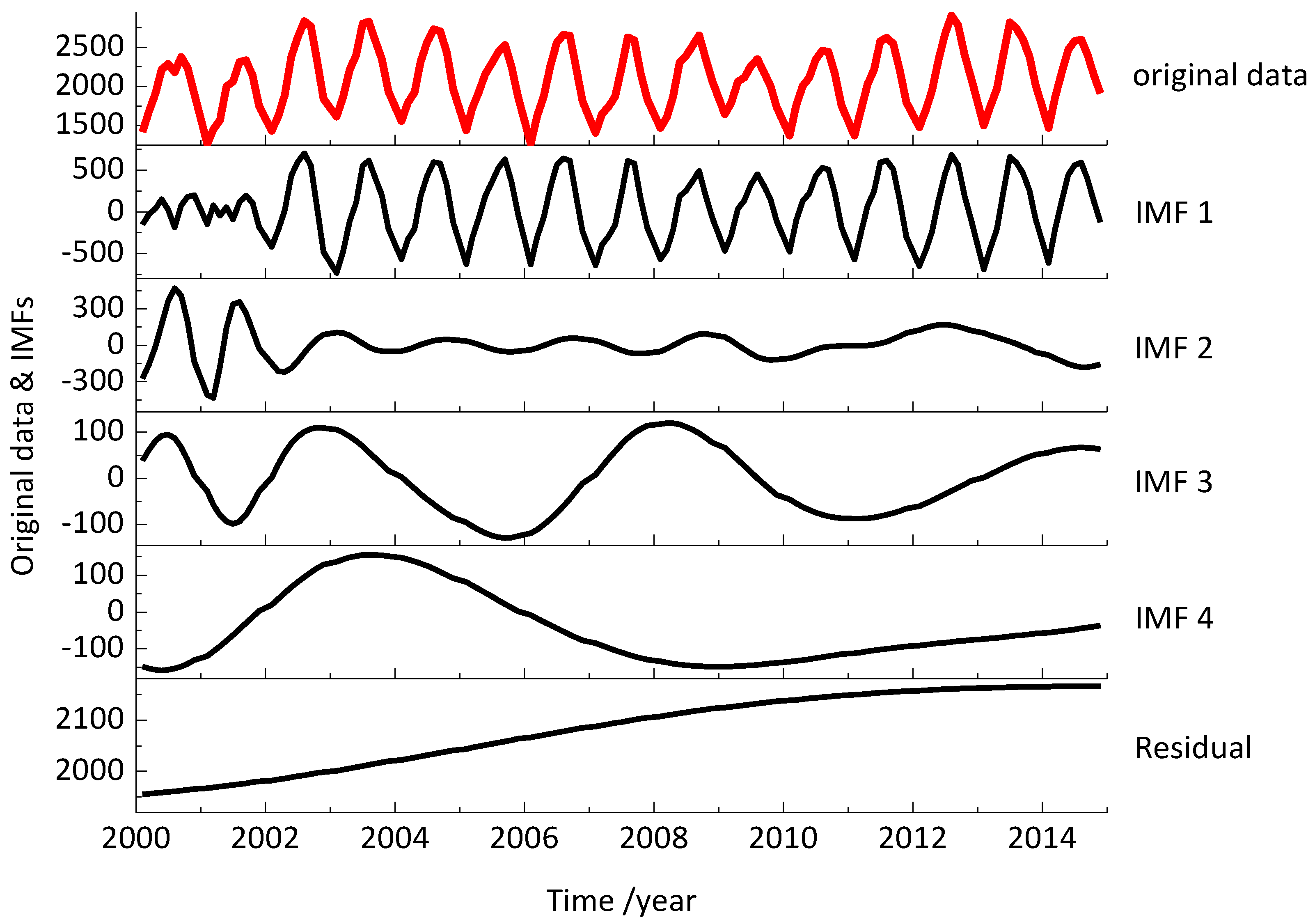
Figure 2. First, we applied Empirical Model Decomposition (EMD) to extract long-term trends of EVI, precipitation, and temperature to investigate the spatial and temporal patterns of primary productivity and climate change. Secondly, we designed two east-to-west transects across the entire study area to examine spatial variations of vegetation response to climate change over different precipitation zones. Thirdly, we analyzed different responses of four types of plant communities over the two east-to-west transects, respectively. Finally, we applied redundancy analysis to explore partial and joint effects of precipitation and temperature on primary productivity and to determine whether the effects of precipitation or temperature, or both, on primary productivity varied regionally or over different types of vegetation.
Fluctuations of vegetation growth and climate change exhibit scale-dependent cycles and a trend [37,46,47]. To understand how these cyclic phenomena and the trend aligning with climate change is a key to reveal how vegetation growth respond to climate change. Algorithms in signal decomposition have been studied to extract the trend of change from non-linear and non-stationary time series data. Martínez and Gilabert [24] successfully detected the dynamics of land cover changes by applying wavelet transformation through normalized deviation vegetation index (NDVI) in inter-annual scale. The basic function, decomposition scale and threshold selection for wavelet transformation are manually set. In addition, these manual settings are multivariate based on specific applications [24]. As a self-adaptive approach, EMD decomposes the non-stationary signal based on its own peculiarity [48]. Kong et al. [39] presented a rigorous decomposition approach for MODIS NDVI with ensemble EMD. In his study, the trend is generated by the combination of lower frequency components decomposed from the original data and the residual which is an overall trend of time series [49]. Wu and Huang [50] claimed that the overall trend that is derived as an intrinsically fitted monotonic function where there can be at most one extremum within a given span. Therefore, in this study, we adopted the residual, the trend of overall time series [39], to analyze vegetation response to climate change.
The algorithm of EMD was originally developed to decompose non-stationary and non-linear signals with several zero mean components [48], which was improved by adding new stopping criteria to make EMD implementation more effective [51]. Rilling’s EMD algorithm code was adapted in this paper. The following is a brief description of the EMD approach. Signal x(t) is the given time series of EVI, or precipitation or temperature (for details, see [51]):
  • Create the top and bottom envelope with the cubic splines fitted by maximums and minimums extras of x(t).
  • Calculate the mean of envelopes: mean(t) = 0.5 × (emax(t) + emin(t)) (where e stands for envelop)
  • Extract the mean value out: x’(t) = x(t) − mean(t)
  • Repeat previous steps until stopping criteria are met and then extract out the intrinsic mode function (IMF): IMF = x(t) − ∑(mean(t))
  • Extract IMF out of x(t): x′ = x(t) − IMF
  • Repeat Steps 1–5 until the criterion that it cannot extract IMFs is met.
  • The residual is what is left: Residual = x(t) − ∑(IMF)
Our research question is whether precipitation or temperature has varied impact on vegetation growth. Pearson’s correlation analysis is often used to test the relationship between one vegetation series and one corresponding environment variable [2]. However, it is long known that climate factors themselves show very interactive and complex correlation. Redundancy analysis (RDA), a special case of Canonical Correspondence Analysis (CCA) that integrates correspondence analysis and multi-variable regression, is currently adopted to test the partial effect of each climate variable on vegetation growth [35,40]. CCA is often used for an analysis where the interested variation is embedded in compositional data and is based on the unimodal model. RDA is typically applied to non-complex data based on the linear model, where the gradient detected by CCA is less than 3 [52]. Han [35] confirmed that the precipitation was a major climate factor affecting vegetation communities in Inner Mongolia through CCA. Sun et al. [40] found that the precipitation was the primary factor in governing the dynamics of vegetation via RDA in Tibetan Plateau. Considering that our data are not composite data, RDA was chosen and applied with the software package CANOCO 5. In other words, we adopted RDA to interpret the relationships between types of vegetation and two climate factors.
RDA is a kind of constrained ordination, first demonstrated by Rao [53], which aims to detect the explanation proportion of the variation of response variable contributed by each explanatory variable [52] (pp. 630). Tsai et al. [54] used RDA to analyze the explanation proportion of climate factors on vegetation change in Taiwan. Moreover, Li et al. [34] found that temperature and rainfall noticeably affect vegetation composition structure through RDA. The explanation proportion is calculated through the following functions
R Y | X 2 = S S ( Y ^ ) S S ( Y )
where R Y | X 2 is the same as R square in multi-variable linear regression (the square of the Pearson’s coefficient), Y is the response matrix with n cases and p response variables, and X is the explanatory matrix with n cases and m explanatory variables. S S ( Y ^ ) is the sum of square of Y ^ (estimated Y through linear regression) and S S ( Y ) is the sum of square of Y (observed values). Notice that S S ( Y ^ )   or S S ( Y ) is sometimes described as sum of squared deviation from mean [52] (pp. 633).
The following is the adjusted R square equation [55], which is also considered as explanatory proportion of X to variance of Y [35].
R a 2 = 1 ( 1 R Y | X 2 ) ( n 1 ) ( n m 1 )
where n is the number of cases in study, and m is the number of explanatory variables. To clarify the statics effectiveness of the adjust R square, also explanation proportion, the F-statistic to test the significant should be conducted as follows [56]:
F = R Y | X 2 m · p ( 1 R Y | X 2 ) ( n m 1 ) p
where p is the number of response variables. Notice that Y here should be the standardized Y (for details, see [52] (pp. 634 [56,57]).
We conducted RDA to analyze the reactions of vegetation to its climate factors in CANOCO, which is effective software for analyzing the relation between a set of environment factors and a set of species in ecology [35,58]. The CANOCO v5 software package is available at http://www.canoco5.com/. Before running the RDA, which is a multivariate regression analysis, the statistical assumptions concerning a regression analysis need to be verified. In CANOCO, partial RDA [59], which is the RDA integrated with variation partitioning analysis, was used to evaluate the marginal explanation rate of precipitation and temperature on EVI variation.

3. Results

3.1. The Result form Empirical Mode Decomposition (EMD)

Long-term trends of change were extracted from the time series of original data through EMD. The outcomes of decomposition processes of EVI are illustrated in Figure 3, using the Steppe grassland as an example. The trends of change from 2000 to 2014 over 135 growth periods are plotted as surfaces along the east–west transection for EVI (Figure 4), precipitation (Figure 5) and temperature (Figure 6).
The spatial pattern of EVI in general increased from west to east (Figure 4). When looking at the bottom of the EVI surface, we clearly found that the western section (the dessert and bare steppe) had the lowest EVI, which indicated poor vegetation growth. Secondly, EVI trends displayed a noticeable increase since 2008, which coincided with the enacting of the grassland conservation compensation policy [16,60]. Although vegetation growth was much better in the eastern section, there were several locations showing relatively lower EVI surfaces, which were overlapping with bare steppe.
Precipitation trend surface was clearly rising from west to the middle position of the transect (Figure 5), indicating the transition from desert to grassland. In addition, the precipitation surface displayed many local fluctuations. For instance, there was a low and flat surface between 4300 and 5000 pixels (one pixel equals 250 m) and several abnormal peaks between 3500 and 4200 pixels from 2010 to 2014. Moreover, it appeared that precipitation showed a general increase in the eastern section in recent years.
The temperature displayed a V-shaped spatial pattern. In the dry western part, temperature change showed a declining trend. It appeared that the drier the location was, the more apparent the declining trend was. However, this finding was different from the study of Chuai et al. [2], which reported an increase in temperature by linear regression of the original time series data. We attributed this difference to the extraction of longitudinal trend of change from the time-series temperature data, since a decreasing trend was also detected when we were running linear regression models. During the section of 4000–5500 pixels, there existed a valley (i.e., where the decreasing trend was apparent). The ground plant covers over this section were the steppe and farmland. The vegetation coverage was very high (Figure 4) in comparison with other sections. It was clear that the trend of temperature change in this section was significantly modified by local vegetation growth condition. The trend of temperature change near the farthest eastern section displayed noticed local variations.

3.2. Partial Effect of Precipitation and Temperature on Productivity at Regional Scale

At the regional scale, we designed two experiments: one aimed to illustrate the advantage of using EMD filtered trend data for regression analysis and the other aimed to reveal possible linear relationships among primary productivity, precipitation and temperature at the regional scale (i.e., in the east and west transects, respectively). In the first experiment, the EVI, precipitation and temperature were averaged across the entire study area, including both west and east transects. The data records were the time-series of 135 16-day periods from 2000 to 2014. To confirm whether the EMD filtered trend dataset was more effective than the original observation dataset, we compared two RDA models, one with the original data and the other with the EMD filtered data. The dependent variable was EVI (the original and the filtered), while the independent variables included the precipitation and temperature (the original and the filtered). The results are included in Table 1 and Table 2. Variation(adj) was the adjusted R square in linear model, which was called the explanatory proportion, referring the variation of EVI explained by the environment variable of interest [52] (pp. 553). Percent of Explained indicated the contribution of each environment variable on the explanation of the EVI variation, i.e., the contribution percentage to the adjusted R square. Percent of All is the product of the explanatory proportion and the percentage of explanation. F and P are the permutation tests of F-static and P-value, indicating whether the model is statistically significant For the joint effect, there are no F and P values, since it does not have the degree of freedom [52].
The total explained Variation(adj) for the original data was 28.14%, which indicated that only 28.14% of the EVI variation could be explained by precipitation, temperature and their joint effect. Thus, the unexplained variation was 71.86%. Under such situation, it was not meaningful to look at the contribution from precipitation or temperature, separately. On the other hand, the RDA model based on the EMD residuals produced a very high total explanatory proportion 0.96 (96%) comparing with 0.28 (28%) from the original data. Moreover, the dominant factor was the joint effect of precipitation and temperature. In fact, a very important finding confirmed that synchronization of rain and heat during growing seasons is the most important condition for high grassland productivity [3]. In addition, precipitation had a higher partial effect (4.2%) than that of temperature (0.9%), which was opposite from the original data result.
To further detect the variation of vegetation growth response to climate change between different climate zones, i.e., between arid and semiarid sections, we ran additional RDA models with the EMD filtered data of EVI, precipitation and temperature over the arid and semiarid sections, respectively. In this part, the precipitation and temperature were calculated by the average values of the east and west transects separately. In other words, the vegetation types were ignored. First, we ran two RDA models using the original data (unfiltered by EMD). The results are reported in Table 3 (Semiarid) and Table 4 (Arid). The finding was similar to those reported in Table 1. The total explained Variation(adj) for the original data over the semiarid transect was 27.96%, while the total explained Variation(adj) over the arid transect was 15.94%. It was very clear that there were no linear relationships in the original datasets. Thus, it was not meaningful to explore linear relationships using the original data. From now on, we focus on the EMD filtered data for further analyses.
The RDA model results from the EMD filtered data are reported in Table 5 (Semiarid) and Table 6 (Arid). Both regional RDA models performed well in terms of explaining the variation of EVI. The total explanation proportions were 97.7% and 98.4% in the semiarid and arid sections, respectively. Regarding individual effect, both precipitation and temperature had higher explanation proportions in the semiarid region than in the arid region. On the other hand, the joint effect in the arid area (86.0%) was much higher than that (40.5%) in the semiarid section, indicating that the synchronization of rain and heat was extremely important to vegetation growth in the arid region.

3.3. Partial Effect of Precipitation and Temperature on Productivity over Different Types of Vegetation Across Two Climate Zones

We examined whether partial effects of precipitation and temperature on primary productivity varied across various types of vegetation and over two climate zones. Table 7 summarizes the RDA analysis for each type of vegetation in the arid (the west) transect and the semiarid (the east) transect, respectively. Prec is the accumulated precipitation and Temp is the average temperature over each type of vegetation in different transects. Percent Explanation is the adjusted explanation proportion of an environment variable upon vegetation productivity (EVI), which is the adjusted R square in linear regression. There are three columns under Partial Effect: partial effect of precipitation, partial effect of temperature and joint effect of both, which reveal the explanation percentage by each of them. Two columns under the Pearson’s Correlation reflect the strength and direction of the relationship between EVI and an environmental factor. A significance test is automatically included in CANOCO 5 software. All analysis outcomes were statistically significant with the confidence level p < 0.05.
Table 7 contains a lot of information. For example, in the arid environment (the west transect), precipitation contributed 6.1% out of the total 97.5% explained variation of Steppe EVI, while temperature contributed 68.3%. Moreover, both correlations had negative signs, which indicated that neither positively affected Steppe EVI. However, in the semiarid environment (the east transect), precipitation contributed 9.3% out of the total 97.5% explained variation of Steppe EVI and the correlation was positive. In particular, Table 7 shows four interesting findings. First, precipitation usually positively affected EVI except for Steppe EVI in Bare Steppe and Desert because steppe plant communities were rarely found in Bare Steppe and Desert environments. Second, temperature in general had negative impacts on EVI but only showed a positive correlation with semiarid desert EVI in the east transect. Third. The joint effect of precipitation and temperature usually explained a large proportion of the variation of EVI explained by the model and often showed positive impacts. Finally, most of the RDA models performed well and explained above 97% of EVI variation, except Desert EVI in the east transect.

4. Discussion

At the regional scale, our results revealed that the RDA model based on the EMD filtered data explained 96.2% of the variation of EVI. Moreover, our findings reinforced that precipitation had strong and positive effect on EVI compared to temperature, indicating that precipitation was the dominant climate factor affecting EVI in the study region. This finding is consistent with several previous studies [2,3,35]. More importantly, we found that the joint effect of precipitation and temperature accounted 94.9% of what was explained by the RDA model (Table 2), which was much higher than each partial effect and revealed that the synchronization of precipitation and temperature was critical to vegetation growth in the study area.
However, after we bisected the transect into the arid and semiarid sections, the results revealed different findings. In the semiarid section, precipitation, temperature and their joint effect all made noticeable contribution to explain the variation proportions of EVI, although the joint effect and precipitation had higher explanation power than temperature did (Table 6). However, the partial effect of precipitation on primary productivity was lower than temperature in the west transect. The joint effect of precipitation and temperature was higher in both regional and transect models, but was much higher (84.6%) in the west transect model. These findings contradict the common understanding that precipitation is the most important factor driving grassland primary productivity. Therefore, there is a need to reiterate that this paper was using the extracted (or filtered) trend data to examine the linear relationship among primary productivity, precipitation and temperature. In other words, all variables considered in the models were the trends of change, which were the inputs for examining the relationship between primary productivity, precipitation and temperature. As revealed in Table 7, the coefficients of Pearson’s Correlation between the trends of EVI and precipitation were in general positive, which indicated that precipitation directly and positively affected EVI. However, the relationship between temperature and EVI was much more complicated. We further examined the unconventional relationship of the trends of change among EVI, precipitation and temperature by plotting the relationship between the EMD filtered residues of precipitation and temperature over 135 periods, as shown in Figure 7. It was clear that temperature was declining during the study period and precipitation was rising in the early period, but declining in the later period (Figure 7a). There existed apparent regional differences. In the west section, from 2000 to 2009, precipitation increased significantly, but temperature slightly declined (Figure 7b). However, after 2009, both precipitation and temperature noticeably decreased. From the perspective of affecting the trend of change of EVI (the bottom residue curve of Figure 3), the filtered trend of temperature was more closely and negatively correlating with the trend of EVI. Furthermore, the correlation plot of precipitation and temperature in the east section showed a smooth curve, but reversing the trend of EVI (Figure 7c). As a result, both trends of precipitation and temperature almost equally affected the trend of EVI, but the trend of precipitation was positively responding, while the trend of temperature was negatively influencing. We were analyzing the relationships among the trends of changes of the variables of interest, not the original observations. Moreover, the signs of the partial or joint effects are important for knowing how each factor affects primary productivity.
The partial effects of precipitation and temperature on EVI clearly varied over different types of vegetation and climate zones. It is worth pointing out that spatial patterns of vegetations in the study area (Figure 1) played an important role. The precipitation was noticeably lower in western Inner Mongolia, where the ecosystems were mainly Desert and Bare Steppe (Figure 1). As the precipitation increased from west to east, the eastern part became obviously wetter, where the steppe and farmland were predominant. The temperature showed a V shape spatial pattern from west to east (Figure 6). It was extremely high in the arid western part, which obviously restrained vegetation growth because a higher temperature would negatively impact plan growth such as reducing the CO2 exchange rate [61]. Due to the extremely low precipitation and high temperature, the desert was mainly located in this section. The temperature was the lowest in the middle part of the transect and became warmer toward the eastern section and the precipitation climbed across the study area (Figure 5). As the temperature and the precipitation became moderate in the middle and eastern areas, the environment was more suitable for steppe growth and farmland plantation. As stated above, the spatial pattern of vegetation communities and their EVI appeared to be determined by the climate factors. When looking at the time axis of Figure 5 and Figure 6, we found that precipitation and temperature displayed an opposite trend of change from 2000 to 2014. The temperature showed a gradual decrease in this period; however, the precipitation increased in most areas, typically before 2008. There was also a noticeable increase in EVI after 2008 [42], which also coincided with the implementation of the grassland conservation compensation policy [16]. We attributed this primary productivity increase to the feedback of vegetation growth to its environment change as well as policy change. The increase of grassland primary productivity due to the policy led to an improvement in evapotranspiration, and, thus, the effectiveness of precipitation [62].
Current literature indicates that different plant communities have diverse responses to climate changes [2,37,38]. Our results across two precipitation transects and over four vegetation communities took this opinion one step further by revealing that the same vegetation also had varied response to rain and heat in different environments (i.e., the arid and semiarid sections in our study). Steppe, for example, has been positively affected by precipitation but negatively affected by temperature. Although, our results confirmed that this conclusion is true in the east section, it was different in the west, where rain and heat both negatively affected Steppe. When we examined the responses of plant communities to regional and local climate factor, we found these differences also exhibited scale dependency. At the regional scale, precipitation and temperature showed negative effects on most vegetation types except Desert, indicating that most vegetation was fragile in the arid area. In the semiarid section, precipitation and temperature displayed positive effect on most vegetation communities, indicating that their interaction in this section provided a moderate environment for vegetation growth. At the local scale, however, temperature seemed negatively correlated with most vegetation (Table 7) and precipitation was usually positively correlated. This finding did not hold at the regional scale.

5. Conclusions

Although precipitation and temperature are two primary factors affecting grassland productivity (EVI as the proxy in this paper), their relationship is not simply linear. Direct analysis of the relationship based on regression models is less applicable. The EMD filtered trend dataset is effective in analyzing relationships in linear model for observations with cyclical fluctuations such as climatic, ecological and environmental data. The RDA model can isolate the partial effect of precipitation and temperature. The integration of the EMD and RDA methods helps examine diverse responses of vegetation growth to climate change and their variations over different precipitation zones and vegetations. The integration also helps assess the impact of policy changes on vegetation growth.
Our results reinforce the previous conclusion that precipitation is the driving factor for vegetation growth in arid and semiarid regions overall. However, there exist noticeable regional and local variations. Especially when we are examining time-series (longitudinal) causal relationships, we should consider that there is one new aspect of relationship between the trends of changes of the variables in research. From the interpretation point of view, we cannot simply conclude which factors exert more influence than others. We need to probe how these trends of changes are interacting or influencing one another. For instance, in this paper, temperature seems to highly and negatively affect primary productivity in arid area because the trends of temperature and EVI are almost reversed. Our results also indicate that the synchronization of precipitation and temperature is critical to vegetation growth in the study area and, especially, in the drier arid section, where the joint effect is much higher than the partial effect of either precipitation or temperature. Furthermore, vegetation growth appears to interact with both climate change and policy intervention in time. After the implementation of grassland conservation and compensation policy, there have been noticeable increases in EVI since 2008, even though the precipitation declined in the west section. Therefore, climate, vegetation growth and policy intervention complexly interact, providing feedbacks to each other. The vegetation communities across the entire study area show varied responses to climate factors, while the same vegetation communities over different climate zones (between the arid and semiarid areas) also display varied responses. In brief, our research extends the knowledge of different responses of vegetation to precipitation and temperature in long-term span across different plant communities and the feedbacks between vegetation growth, climate change and policy intervention. The integration of EMD filtering algorithm and RDA model provides a new effective way to reveal the mechanism of vegetation response to climate change.
Finally, there are several improvements that could be implemented in the future to provide a more comprehensive analysis of vegetation response to climate change and policy intervention. First, at least one policy variable in the form of implementation variation should be considered. The policy of ecosystem compensation and conservation includes three levels: reducing grazing, seasonally shifting grazing and abandoning grazing. Different levels of compensation and conservation incentives will lead to different effects, which should be examined in future analysis. Second, the inclusion of socioeconomic factors should be considered. Vegetation growth is influenced by coupled effect of climate change and socioeconomic transformation [13]. Simply differentiating partial effect of precipitation and temperature is too limited to the out true vegetation responses to coupled human and nature systems.

Author Contributions

Conceptualization, Y.X. and T.C.; Methodology, T.C. and C.L.; Software, T.C. and L.M.; Formal Analysis, Y.X. and T.C.; Investigation, Y.X. and T.C.; Resources, S.F. and L.M.; Data Curation, T.C., L.M. and S.F.; Writing-Original Draft Preparation, T.C.; Writing-Review & Editing, Y.X., Y.B. and A.Z.; Visualization, T.C.; Supervision, Y.X.; Project Administration, Y.X.; Funding Acquisition, Y.X.

Acknowledgments

Guangdong Innovative and Entrepreneurial Research Team Program, 2016ZT06D336; GDAS' Special Project of Science and Technology Development, 2017GDASCX-0101

Conflicts of Interest

The authors declare no conflicts of interest.

References

  1. Bao, G.; Qin, Z.; Bao, Y.; Zhou, Y.; Li, W.; Sanjjav, A. NDVI-based long-term vegetation dynamics and its response to climatic change in the Mongolian plateau. Remote Sens. 2014, 6, 8337–8358. [Google Scholar] [CrossRef]
  2. Chuai, X.; Huang, X.; Wang, W.; Bao, G. NDVI, temperature and precipitation changes and their relationships with different vegetation types during 1998–2007 in Inner Mongolia, China. Int. J. Climatol. 2013, 33, 1696–1706. [Google Scholar] [CrossRef]
  3. Bai, Y.; Wu, J.; Xing, Q.; Pan, Q.; Huang, J.; Yang, D.; Han, X. Primary production and rain use efficiency across a precipitation gradient on the Mongolia plateau. Ecology 2008, 89, 2140–2153. [Google Scholar] [CrossRef] [PubMed]
  4. Balling, R.C.; Klopatek, J.M.; Hildebrandt, M.L.; Moritz, C.K.; Watts, C.J. Impacts of land degradation on historical temperature records from the Sonoran desert. Clim. Change 1998, 40, 669–681. [Google Scholar] [CrossRef]
  5. Grime, J.P.; Fridley, J.D.; Askew, A.P.; Thompson, K.; Hodgson, J.G.; Bennett, C.R. Long-term resistance to simulated climate change in an infertile grassland. Proc. Natl. Acad. Sci. USA 2008, 105, 10028–10032. [Google Scholar] [CrossRef] [PubMed] [Green Version]
  6. Pielke, R.; Schimel, D.; Lee, T.; Kittel, T.; Zeng, X. Atmosphere-terrestrial ecosystem interactions: Implications for coupled modeling. Ecol. Model. 1993, 67, 5–18. [Google Scholar] [CrossRef]
  7. Piras, M.; Mascaro, G.; Deidda, R.; Vivoni, E.R. Impacts of climate change on precipitation and discharge extremes through the use of statistical downscaling approaches in a Mediterranean basin. Sci. Total Environ. 2016, 543, 952–964. [Google Scholar] [CrossRef] [PubMed]
  8. Gong, Z.; Ito, Y.; Kawamura, K.; Ishikawa, N.; Goto, M.; Wulan, T.; Alateng, D.; Yin, T. MODIS NDVI and vegetation phenology dynamics in the Inner Mongolia grassland. Solid Earth Discuss. 2015, 7. [Google Scholar] [CrossRef]
  9. Li, S.; Xie, Y.; Brown, D.G.; Bai, Y.; Hua, J.; Judd, K. Spatial variability of the adaptation of grassland vegetation to climatic change in Inner Mongolia of China. Appl. Geogr. 2013, 43, 1–12. [Google Scholar] [CrossRef]
  10. Xie, Y.; zhang, Y.; Lan, H.; Mao, L.; Zeng, S.; Chen, Y. Investigating long-term trends of climate change and their spatial variations caused by regional and local environments through data mining. J. Geogr. Sci. 2018, 28, 802–818. [Google Scholar] [CrossRef]
  11. Solomon, S.; Qin, D.; Manning, M.; Chen, Z.; Marquis, M.; Averyt, K.B.; Tignor, M.; Miller, H.L. Contribution of Working Group I to the Fourth Assessment Report of the Intergovernmental Panel on Climate Change, 2007; Cambridge University Press: Cambridge, UK, 2007. [Google Scholar]
  12. Shiyomi, M.; Akiyama, T.; Wang, S.; Hori, Y.; Chen, Z.; Yasuda, T.; Kawamura, K.; Yamamura, Y. A grassland ecosystem model of the Xilingol steppe, Inner Mongolia, China. Ecol. Model. 2011, 222, 2073–2083. [Google Scholar] [CrossRef]
  13. Xie, Y.; Crary, D.; Bai, Y.; Cui, X.; Zhang, A. Modeling grassland ecosystem responses to coupled climate and socioeconomic influences in multi-spatial-and-temporal scales. J. Environ. Inform. 2017. [Google Scholar] [CrossRef]
  14. Damsø, T.; Kjær, T.; Christensen, T.B. Local climate action plans in climate change mitigation: examining the case of Denmark. Energy Policy 2016, 89, 74–83. [Google Scholar] [CrossRef]
  15. Chen, L.; Li, H.; Zhang, P.; Zhao, X.; Zhou, L.; Liu, T.; Hu, H.; Bai, Y.; Shen, H.; Fang, J. Climate and native grassland vegetation as drivers of the community structures of shrub-encroached grasslands in Inner Mongolia, China. Landsc. Ecol. 2015, 30, 1627–1641. [Google Scholar] [CrossRef]
  16. Brown, D.G.; Agrawal, A.; Sass, D.A.; Wang, J.; Hua, J.; Xie, Y. Responses to climate and economic risks and opportunities across national and ecological boundaries: Changing household strategies on the Mongolian plateau. Environ. Res. Lett. 2013, 8, 045011. [Google Scholar] [CrossRef] [PubMed]
  17. Yuan, X.; Li, L.; Chen, X.; Shi, H. Effects of precipitation intensity and temperature on NDVI-based grass change over northern China during the period from 1982 to 2011. Remote Sens. 2015, 7, 10164–10183. [Google Scholar] [CrossRef]
  18. Lu, N. Regional Climate Change and Vegetation-Water Relations in Inner Mongolia Lessons Learned within the Nasa Project “Effects of Land Use Change on the Energy and Water Balance of the Semi-Arid Region of Inner Mongolia, China”; The University of Toledo: Toledo, OH, USA, 2009. [Google Scholar]
  19. Parrott, L.; Meyer, W.S. Future landscapes: Managing within complexity. Front. Ecol. Environ. 2012, 10, 382–389. [Google Scholar] [CrossRef]
  20. Stiles, A.; Scheiner, S.M. A multi-scale analysis of fragmentation effects on remnant plant species richness in Phoenix, Arizona. J. Biogeogr. 2010, 37, 1721–1729. [Google Scholar] [CrossRef]
  21. Chamaillé-Jammes, S.; Fritz, H. Precipitation–NDVI relationships in eastern and southern African savannas vary along a precipitation gradient. Int. J. Remote Sens. 2009, 30, 3409–3422. [Google Scholar] [CrossRef]
  22. Guan, B.T. Ensemble empirical mode decomposition for analyzing phenological responses to warming. Agric. For. Meteorol. 2014, 194, 1–7. [Google Scholar] [CrossRef]
  23. Hawinkel, P.; Swinnen, E.; Lhermitte, S.; Verbist, B.; Van Orshoven, J.; Muys, B. A time series processing tool to extract climate-driven interannual vegetation dynamics using ensemble empirical mode decomposition (EEMD). Remote Sens. Environ. 2015, 169, 375–389. [Google Scholar] [CrossRef] [Green Version]
  24. Martínez, B.; Gilabert, M.A. Vegetation dynamics from NDVI time series analysis using the wavelet transform. Remote Sens. Environ. 2009, 113, 1823–1842. [Google Scholar] [CrossRef]
  25. Fan, J.; Wang, K.; Harris, W.; Zhong, H.; Hu, Z.; Han, B.; Zhang, W.; Wang, J. Allocation of vegetation biomass across a climate-related gradient in the grasslands of Inner Mongolia. J. Arid Environ. 2009, 73, 521–528. [Google Scholar] [CrossRef]
  26. Briske, D.D.; Zhao, M.; Han, G.; Xiu, C.; Kemp, D.R.; Willms, W.; Havstad, K.; Kang, L.; Wang, Z.; Wu, J. Strategies to alleviate poverty and grassland degradation in Inner Mongolia: Intensification vs production efficiency of livestock systems. J. Environ. Manag. 2015, 152, 177–182. [Google Scholar] [CrossRef] [PubMed]
  27. Gisladottir, G.; Stocking, M. Land degradation control and its global environmental benefits. Land Degrad. Dev. 2005, 16, 99–112. [Google Scholar] [CrossRef]
  28. Xie, Y.; Sha, Z.; Yu, M.; Bai, Y.; Zhang, L. A comparison of two models with Landsat data for estimating above ground grassland biomass in Inner Mongolia, China. Ecol. Model. 2009, 220, 1810–1818. [Google Scholar] [CrossRef]
  29. Liu, J.; Dietz, T.; Carpenter, S.R.; Alberti, M.; Folke, C.; Moran, E.; Pell, A.N.; Deadman, P.; Kratz, T.; Lubchenco, J. Complexity of coupled human and natural systems. Science 2007, 317, 1513–1516. [Google Scholar] [CrossRef] [PubMed]
  30. Wang, Z.; Deng, X.; Song, W.; Li, Z.; Chen, J. What is the main cause of grassland degradation? A case study of grassland ecosystem service in the middle-south Inner Mongolia. Catena 2017, 150, 100–107. [Google Scholar] [CrossRef]
  31. Zhao, X.; Hu, H.; Shen, H.; Zhou, D.; Zhou, L.; Myneni, R.B.; Fang, J. Satellite-indicated long-term vegetation changes and their drivers on the Mongolian plateau. Landsc. Ecol. 2015, 30, 1599–1611. [Google Scholar] [CrossRef]
  32. Guo, L.; Wu, S.; Zhao, D.; Yin, Y.; Leng, G.; Zhang, Q. NDVI-based vegetation change in Inner Mongolia from 1982 to 2006 and its relationship to climate at the biome scale. Adv. Meteorol. 2014, 2014. [Google Scholar] [CrossRef]
  33. Li, A.; Wu, J.; Huang, J. Distinguishing between human-induced and climate-driven vegetation changes: A critical application of restrend in Inner Mongolia. Landsc. Ecol. 2012, 27, 969–982. [Google Scholar] [CrossRef]
  34. Li, Z.; Ma, W.; Liang, C.; Liu, Z.; Wang, W.; Wang, L. Long-term vegetation dynamics driven by climatic variations in the Inner Mongolia grassland: Findings from 30-year monitoring. Landsc. Ecol. 2015, 30, 1701–1711. [Google Scholar] [CrossRef]
  35. Han, F.; Kang, S.; Buyantuev, A.; Zhang, Q.; Niu, J.; Yu, D.; Ding, Y.; Liu, P.; Ma, W. Effects of climate change on primary production in the Inner Mongolia plateau, China. Int. J. Remote Sens. 2016, 37, 5551–5564. [Google Scholar] [CrossRef]
  36. Zhang, G.; Xu, X.; Zhou, C.; Zhang, H.; Ouyang, H. Responses of grassland vegetation to climatic variations on different temporal scales in Hulun Buir grassland in the past 30 years. J. Geogr. Sci. 2011, 21, 634–650. [Google Scholar] [CrossRef]
  37. Leemans, R.; Eickhout, B. Another reason for concern: Regional and global impacts on ecosystems for different levels of climate change. Glob. Environ. Change 2004, 14, 219–228. [Google Scholar] [CrossRef]
  38. Puntsukova, S.D.; Gomboev, B.O.; Akhmetzyanova, M.R.; Jamsran, T.; Dagdan, T.; Suocheng, D. Comparative analysis of different forest ecosystems response to global climate change and economic activity. J. Resour. Ecol. 2015, 6, 106–109. [Google Scholar] [CrossRef]
  39. Kong, Y.-L.; Meng, Y.; Li, W.; Yue, A.-Z.; Yuan, Y. Satellite image time series decomposition based on EEMD. Remote Sens. 2015, 7, 15583–15604. [Google Scholar] [CrossRef]
  40. Sun, J.; Qin, X.; Yang, J. The response of vegetation dynamics of the different alpine grassland types to temperature and precipitation on the Tibetan plateau. Environ. Monit. Assess. 2016, 188, 20. [Google Scholar] [CrossRef] [PubMed]
  41. Chen, X.; Vierling, L.; Deering, D. A simple and effective radiometric correction method to improve landscape change detection across sensors and across time. Remote Sens. Environ. 2005, 98, 63–79. [Google Scholar] [CrossRef]
  42. Bai, Y.; Wu, J.; Pan, Q.; Huang, J.; Wang, Q.; Li, F.; Buyantuyev, A.; Han, X. Positive linear relationship between productivity and diversity: Evidence from the Eurasian steppe. J. Appl. Ecol. 2007, 44, 1023–1034. [Google Scholar] [CrossRef]
  43. Wilcox, D.A.; Xie, Y. Predicted effects of proposed new regulation plans on sedge/grass meadows of Lake Ontario. J. Great Lakes Res. 2008, 34, 745–754. [Google Scholar] [CrossRef]
  44. Jing, W.; Yang, Y.; Yue, X.; Zhao, X. A spatial downscaling algorithm for satellite-based precipitation over the Tibetan plateau based on NDVI, DEM, and land surface temperature. Remote Sens. 2016, 8, 655. [Google Scholar] [CrossRef]
  45. Wang, J.; Rich, P.M.; Price, K.P. Temporal responses of NDVI to precipitation and temperature in the central Great Plains, USA. Int. J. Remote Sens. 2003, 24, 2345–2364. [Google Scholar] [CrossRef] [Green Version]
  46. Kardol, P.; Cregger, M.A.; Campany, C.E.; Classen, A.T. Soil ecosystem functioning under climate change: Plant species and community effects. Ecology 2010, 91, 767–781. [Google Scholar] [CrossRef] [PubMed]
  47. Xie, Y.; Sha, Z.; Yu, M. Remote sensing imagery in vegetation mapping: A review. J. Plant Ecol. 2008, 1, 9–23. [Google Scholar] [CrossRef]
  48. Huang, N.E.; Shen, Z.; Long, S.R.; Wu, M.C.; Shih, H.H.; Zheng, Q.; Yen, N.-C.; Tung, C.C.; Liu, H.H. In The Empirical Mode Decomposition and the Hilbert Spectrum for Nonlinear and Non-Stationary Time Series Analysis. In Proceedings of the Royal Society of London A: Mathematical, Physical and Engineering Sciences, London, UK, 8 March 1998; The Royal Society: London, UK, 1998; pp. 903–995. [Google Scholar]
  49. Wu, Z.; Huang, N.E.; Long, S.R.; Peng, C.-K. On the trend, detrending, and variability of nonlinear and nonstationary time series. Proc. Natl. Acad. Sci. USA 2007, 104, 14889–14894. [Google Scholar] [CrossRef] [PubMed] [Green Version]
  50. Wu, Z.; Huang, N.E. Ensemble empirical mode decomposition: A noise-assisted data analysis method. Adv. Adapt. Data Anal. 2009, 1, 1–41. [Google Scholar] [CrossRef]
  51. Rilling, G.; Flandrin, P.; Goncalves, P. On Empirical Mode Decomposition and Its Algorithms. In Proceedings of the IEEE-EURASIP Workshop on Nonlinear Signal and Image Processing, NSIP-03, Grado, Italy, 8–11 June 2003; pp. 8–11. [Google Scholar]
  52. Legendre, P.; Legendre, L.F. Numerical Ecology; Elsevier: New York, NY, USA, 2012; Volume 24. [Google Scholar]
  53. Rao, C.R. The use and interpretation of principal component analysis in applied research. Sankhyā Indian J. Stat. Ser. A 1964, 26, 329–358. [Google Scholar]
  54. Tsai, H.P.; Lin, Y.-H.; Yang, M.-D. Exploring Long Term Spatial Vegetation Trends in Taiwan from AVHRR NDVI3g Dataset Using RDA and HCA Analyses. Remote Sens. 2016, 8, 290. [Google Scholar] [CrossRef]
  55. Ezekiel, M. Methods of Correlation Analysis; John Wiley & Sons Inc.: Hoboken, NJ, USA, 1941. [Google Scholar]
  56. Miller, J.K. The sampling distribution and a test for the significance of the bimultivariate redundancy statistic: A Monte Carlo study. Multivar. Behav. Res. 1975, 10, 233–244. [Google Scholar] [CrossRef]
  57. Legendre, P.; Oksanen, J.; ter Braak, C.J. Testing the significance of canonical axes in redundancy analysis. Methods Ecol. Evol. 2011, 2, 269–277. [Google Scholar] [CrossRef]
  58. McKee, A.; Lake Huron, C.; Midwood, J.; Chow-Fraser, P. Water-Level-Induced Changes in Fish Communities in Coastal Wetlands of Eastern Georgian Bay; Upper Great Lakes Management Unit, Ontario Ministry of Natural Resources: Owen Sound, ON, Canada, 2010. [Google Scholar]
  59. Davies, P. Procedures for reduced-rank regression. Appl. Stat. 1982, 31, 244–255. [Google Scholar] [CrossRef]
  60. Hao, L.; Sun, G.; Liu, Y.; Gao, Z.; He, J.; Shi, T.; Wu, B. Effects of precipitation on grassland ecosystem restoration under grazing exclusion in Inner Mongolia, China. Landsc. Ecol. 2014, 29, 1657–1673. [Google Scholar] [CrossRef]
  61. He, X.; He, K.S.; Hyvönen, J. Will bryophytes survive in a warming world? Perspect. Plant Ecol. Evol. Syst. 2016, 19, 49–60. [Google Scholar] [CrossRef]
  62. Wu, M.; Schurgers, G.; Rummukainen, M.; Smith, B.; Samuelsson, P.; Jansson, C.; Siltberg, J.; May, W. Vegetation-climate feedbacks modulate rainfall patterns in Africa under future climate change. Earth Syst. Dyn. 2016, 7, 627–647. [Google Scholar] [CrossRef]
Figure 1. The study area of Inner Mongolia Plateau and the east–west transects.
Ijgi 07 00214 g001
Figure 2. Flow chart of the synthesized research design and method.
Ijgi 07 00214 g002
Figure 3. Original time series and EMD intrinsic fractions (including residual) of the EVI of Steppe Grassland, 2000–2014.
Ijgi 07 00214 g003
Figure 4. EVI residuals displayed in spatial and temporal surface.
Ijgi 07 00214 g004
Figure 5. Precipitation residuals displayed in spatial and temporal surface.
Ijgi 07 00214 g005
Figure 6. Temperature residuals displayed in spatial and temporal surface.
Ijgi 07 00214 g006
Figure 7. Relation between temperature and precipitation after EMD extraction. (a) the entire region; (b) the west transect; (c) the east transect.
Ijgi 07 00214 g007
Table 1. RDA Results for the original data at regional scale.
FractionVariation (adj)Percent of ExplainedFP
Precipitation0.04982117.71450.002
Temperature0.1119439.833.10.002
Joint effect0.1196742.5
Total Explained0.28143100.0
All Variation1
Correlation of predictors0.482759
Table 2. RDA Results for EMD residuals at regional scale.
FractionVariation (adj)Percent of ExplainedFP
Precipitation0.0402494.21450.002
Temperature0.00893560.933.10.002
Joint effect0.9137494.9
Total Explained0.96293100.017410.002
All Variation1 134
Table 3. Outcomes of RDA model (Original) over the semiarid transect.
FractionVariation (adj)% of ExplainedFP
Precipitation0.04348115.627.00.001
Temperature0.1059537.99.00.002
Joint Effect0.1301546.6
Total Explained0.27957100.020.60.001
All Variation1
Correlation of predictors 0.493891
Table 4. Outcomes of RDA model (Original) over the arid transect.
FractionVariation (adj)% of ExplainedFP
Precipitation0.0321920.26.10.006
Temperature0.1206875.720.10.001
Joint Effect0.00647894.1
Total Explained0.15935100.013.70.001
All Variation1
Correlation of predictors 0.07562
Table 5. Outcomes of RDA model(EMD) over the semiarid transect.
FractionVariation (adj)% of ExplainedFP
Precipitation0.3174832.514570.02
Temperature0.254626.118160.02
Joint Effect0.4046641.4
Total Explained0.97674100.028410.02
All Variation1
Correlation of predictors −0.99382
Table 6. Outcomes of RDA model(EMD) over the arid transect. .
FractionVariation (adj)% of ExplainedFP
Precipitation0.04684.83800.3
Temperature0.077097.86250.362
Joint Effect0.8596987.4
Total Explained0.98358100.040140.04
All Variation1
Correlation of predictors −0.97398
Table 7. Outcomes of RDA models over two transects and four plant communities.
EVI by Vegetation TypeTran-Sect%ExplanationPartial EffectPearson’s CorrelationPredictors
Correlation
Significance
PrecTempJointPrecTempFP
Steppewest97.56.168.325.7−0.56−0.970.8826170.002
east97.59.3090.70.99−0.94−0.6725790.004
Farmlandwest99.913.792.1−5.90.29−0.93−0.99741070.002
east97.422.64.872.60.96−0.88−0.0624920.002
Barewest99.90.499.30.3−0.12−0.99−0.56676110.002
east99.73.915.680.40.91−0.980.89286460.002
Gobi/desertwest98.61.95.091.70.97−0.99−0.9448300.002
east85.395100.8−96.00.020.23−0.373900.002

